1. Introduction
When James Clerk Maxwell introduced the displacement current as a property of empty space and as a source of magnetic field, he struck gold. The result was his famous set of self-consistent equations, which later even turned out to be Lorentz invariant and describe electromagnetism with greatest precision.
Maxwell was visualizing the displacement current as part of the ether [
1], an all-pervading medium composed of a subtle substratum. This is a powerful explanatory concept that goes back to the prehistory of science and helped unify our understanding of the physical world for centuries [
2]. However, the ether was soon abandoned as a consequence of Albert Einstein’s special theory of relativity, which contradicts an absolute reference frame, and the vacuum was considered void (nonetheless, Einstein’s relationship with the ether was complex, and changed over time [
3]). However, this move was merely an elegant paradigm shift rather than a necessity forced by observation.
Electrodynamics was the new theory of electromagnetic fields interacting with the—at the time—newly discovered elementary particle, the electron. Already then, cumbersome divergences were looming around the corner and we are struggling with them ever since. One was the question whether or not the electron has a finite radius, and if it does not, as hinted by all experiments at higher and higher energies (or, rather, momentum exchange), then the mass diverges and even the charge of the electron diverges on small enough length scales [
4]. Another such early divergence was discovered by Max Planck [
5]. Previously, he had postulated that the energy had to be quantized in packets of
per mode to derive his famous blackbody radiation formula, where
h is the Planck constant and
is the electromagnetic radiation frequency. However, in 1912, when going to the asymptotic limit for long wavelengths or high temperatures and match it with the experimental observations, Planck noticed that there was an additional contribution
to the energy per mode—this is the first time the ground state energy of a quantum harmonic oscillator appeared in the literature.
Later, after Paul Dirac [
6] hypothesized the existence of the antielectron, later called positron, and its subsequent experimental discovery, scientists struggled in vain for years to formulate a consistent quantum theory of electrodynamics. The breakthrough came when Richard Feynman [
7] and Julian Schwinger [
8] used their approach to first postulate Maxwell’s equations and then added the interaction with electrons and positrons [
9]: modern quantum electrodynamics (QED) was born. By using the procedure of renormalization, the divergences were modified to much better behaved logarithmic divergences. More elementary particles were discovered, including charged ones, and QED is overall highly successful, but some struggle with divergences remains.
Within the framework of QED, it is understood that the quantum vacuum is not void. By now, there is ample experimental evidence for the nonzero ground state energies of quantum fields populating the vacuum, containing the seeds of multiple virtual processes [
10,
11,
12]. Wilczek [
13] expresses the fundamental characteristics of space and time as properties of the ‘grid’, the entity one perceives as empty space. The deepest physical theories reveal it to be highly structured; indeed, it appears as the primary ingredient of reality. Several effects manifest themselves when the vacuum is perturbed in specific ways: vacuum fluctuations lead to shifts in the energy level of atoms [
14], changes in the boundary conditions produce particles [
15], and accelerated motion [
16] and gravitation [
17] can create thermal radiation. A careful discussion of the nature of these ‘vacuum fluctuations’ can be found in [
18], although we think that, perhaps, the ‘vacuum uncertainty’ would be a better term.
Since this quantum vacuum is not void any more, it is natural to mull over the prospect of treating it as a medium with electric and magnetic polarizability. This idea can be traced back as far as Furry and Oppenheimer [
19], Weisskopf and Pauli [
20,
21] (see English translation in Ref. [
22]), Dicke [
23], and Heitler [
24].
At this point one might wonder about how the linear response of the quantum vacuum, which one might—but does not have to—relate to a modern Lorentz-invariant ether, is contained in Maxwell’s [
25]. As this linear response is thought to be already included in Maxwell’s equations and since they were axiomatically postulated, the linear response is not explicitly considered anymore in QED. Along this line of thinking, Maxwell’s equations already contain the effect of the bare vacuum and only the so-called off-shell contributions will still have to be explicitly considered in QED. Details are given below.
Thus, here, we interpret the response of the bare vacuum as caused in full by the vacuum polarization, i.e., the on-shell contribution. This contribution, however, diverges when attempting to determine it in the frame of QED: when calculating the bare vacuum contribution to Maxwell’s equations using the standard QED procedure we do find a closed mathematical expression dependent only on the off-shell momentum value at which the electromagnetic coupling strength diverges.
In an attempt to do a back-of-the-envelope calculation, in this paper, we find a reasonable way to cope with the divergences. This crude derivation uses a relativistic momentum cutoff [
23], similar to the one used by Bethe [
26] to calculate the Lamb shift in hydrogen. It is surprising how well this works. The numbers come out in the right ballpark.
At face value, Maxwell’s equations in vacuum are about electromagnetic fields and the coupling strength between fields and charged particles should not be relevant. However, in the spirit of the discussion above, there is interaction with the vacuum uncertainty, i.e., with virtual electron–positron pairs, and this determines the values of the vacuum permittivity,
, and permeability,
. Thus the coupling strength matters also here. Traditionally, the QED coupling strength is given by Sommerfeld’s fine structure constant,
, in SI units (International System of Units), with
e denoting the electron charge. In Maxwell’s equations it is somewhat hidden, but it is there [
27]. The parameter
refers to the limiting speed in special relativity and not necessarily denotes the speed of light, for the purpose of the derivation here. In this paper, we elaborate on the above ideas and show that
and
can be estimated from first principles and, thus, also the speed of light.
2. A Dielectric Model of Vacuum Polarization
In textbooks of electromagnetism it is often implicitly assumed that and are merely measurement system constants. In this vein, they are not considered as fundamental physical properties, but rather artifacts of the SI units, which disappear in Gaussian units. However, this quite simplified viewpoint ignores that, irrespective of the method of allocating a value to and , they just translate into the prediction of Maxwell’s equations that, in free space, electromagnetic waves propagate at the speed of light, which has a very specific value and is certainly associated with units. It is therefore more transparent if one includes the susceptibility of the vacuum , so that in the vacuum Maxwell’s displacement reads as . In the SI system all the dimensions and the numerical value is put into such that . In comparison, in the Gaussian system of units, is likewise chosen to be ‘one’ and one might say that the modified definition of the electric field absorbs the properties of the vacuum unit in this case. So, for the vacuum one has and the vacuum response is actually hidden in the Gaussian units. In what follows, we use SI units only and the vacuum response is given by the product, . Only the product of the two factors has physical significance and writing this as two factors was a result of the historical development.
In a dielectric, it is customary to define the electric displacement
and the magnetic field
as
where
is the polarization and
the magnetization induced by the external fields with
and
t denoting the position and time, respectively. In the literature, one can find the observation that
and
are the sum of two completely different physical quantities [
28]. However, the authors do not share this view and interpret
and
as the polarization and magnetization of the vacuum, in this sense we are adding similar quantities. This might appear preposterous in classical electromagnetism, but, as declared in
Section 1, the modern view [
29] interprets that particle–antiparticle pairs are continually being created in a vacuum filled with the vacuum fluctuations. They live for a brief period of time and then annihilate each other. The lifetime of such a virtual particle pair is governed by its rest energy through the energy–time uncertainty principle [
30,
31],
where
is the root-mean-square measure of energy nonconservation and
the time interval, during which this nonconservation is sustained. The creation of this virtual pair requires a surplus energy of at least
, where
m is the mass of each partner (we stress again that here
is the limiting speed appearing in Lorentz transformations. After all, in this paper, we want to calculate
and
based on the properties of the vacuum, and this results then in a value of the speed of light based only on these properties of the vacuum. If the result of the crude model here is found to be close to the known value of the speed of light, this will be an indication of the relevance of the enough simple model).
Therefore, energy conservation must be violated by
. Equation (
2) says that the violation is not detectable in a period shorter than
(with
ℏ the reduced Planck’s constant), so virtual particles can survive about that long. However, nothing can move faster than the relativistic speed limit, so the virtual pair must remain within a distance
; that is, a distance of order of the Compton wavelength,
This also demonstrates that heavy pairs require a larger and thus their effect is concentrated at smaller distances. For that reason, let us so far consider only electron–positron pairs.
In the linear response, one expresses the polarization of matter,
, in terms of the corresponding matter susceptibility,
:
(and, similarly, for the magnetization) with
the wave angular frequency. Whenever a medium is dispersive, the linear response is nonlocal in time and integration over past times is required. However, the linear response is local in the frequency domain. Therefore, in order to account for dispersion in the simplest way, let us express the linear response in the frequency domain [
32].
As noticed above, in Equation (
1), the first term is expected to have an equivalent structure:
The vacuum has no resonances and it is homogeneous. The conservation of momentum prohibits the excitation of a virtual pair to a real pair in free space with a plane wave. Far away from resonance, the process is allowed because of the quantum uncertainty of the momentum. In contradistinction, a converging electromagnetic dipole wave may excite real pairs in the vacuum [
33]. So, under normal conditions,
has no temporal or spatial frequency dependence and is considered a constant in classical electromagnetism. Historically, as emphasized above, it was chosen to be unity and all the property of the vacuum such as units and numerical value is put into
. Therefore, the familiar expression for
is
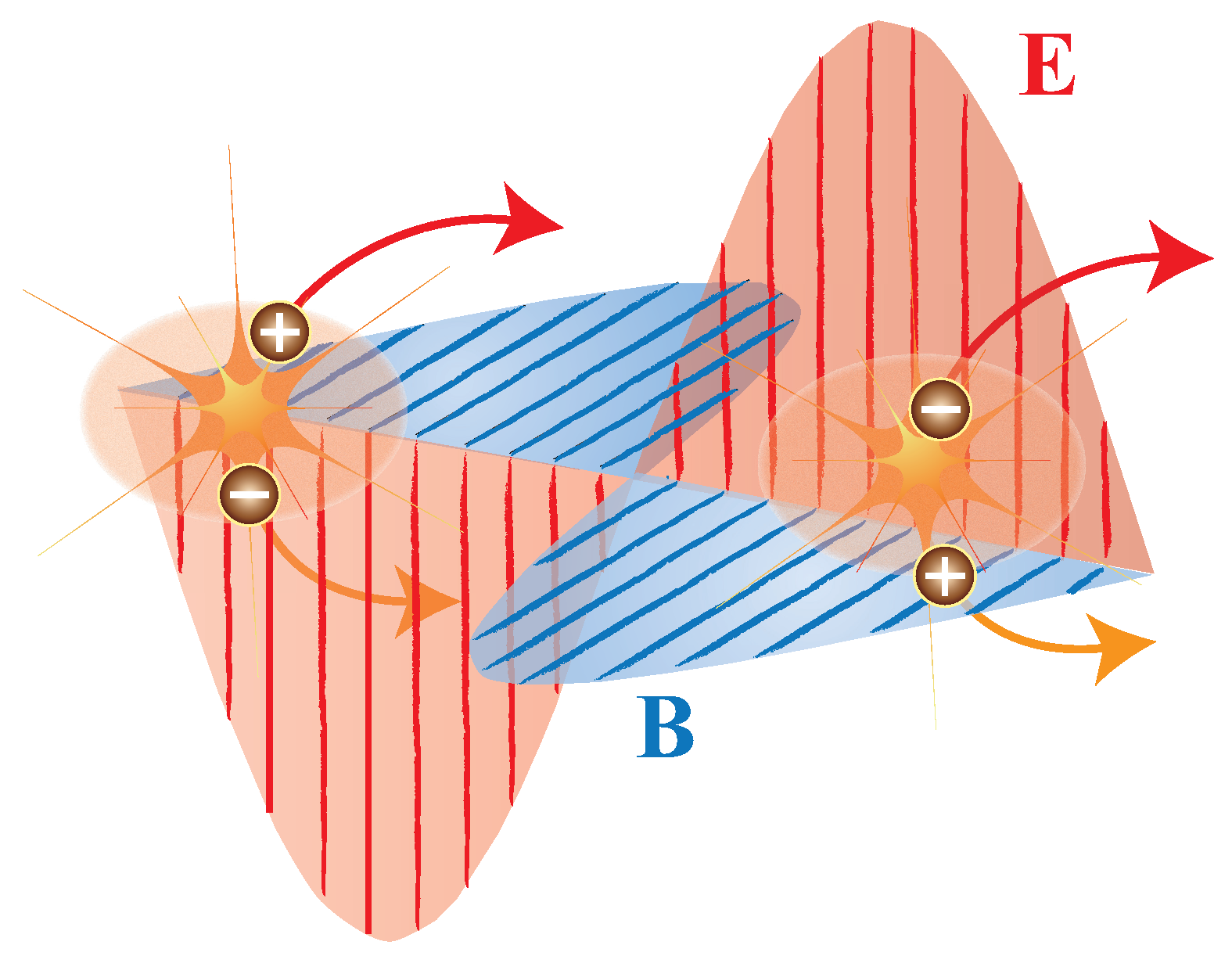
If the value of
is determined by the structure of the vacuum, it should be possible to calculate it by examining the (polarizing) interaction of photons introduced into the vacuum as test particles [
18], as sketched in
Figure 1. The possibility that a charged pair can form an atomic bound state (the electron–positron vacuum fluctuation in the lowest energy level at
that has zero angular momentum is called parapositronium, which is a singlet spin state [
34,
35]), which can, thus, be well approximated by an oscillator, was discussed by Ruark [
36] and further elaborated by Wheeler [
37].
These ideas have recently been readressed [
38,
39,
40,
41] to calculate ab initio
by using methods similar to those employed to determine the permittivity in a dielectric. As it is known [
42], when interacting with an electric field, an atom in its ground state interacts with the electric field as if it were a harmonic oscillator. Here, we adopt the same strategy to treat the virtual pairs composing the vacuum. This is a reasonable assumption as long as deviations from the equilibrium under the action of an electric or magnetic field are tiny, as they are for the vacuum under normal conditions in a low-energy optics laboratory. In this situation, one can do a Taylor expansion around the point of equilibrium and the harmonic response will dominate. The only parameter needed is the charge of the elementary particles and the effective frequency of the oscillator. The latter is given by the ‘spring constant’, i.e., the energy gap between the ground state of a virtual pair and first excited level [
25,
38], where the particles are real. This gap is twice the rest-mass energy,
, of one of the elementary particles of mass
m. No other assumptions are required.
The harmonic oscillator assumption allows one to calculate both the induced electric dipoles and magnetic dipoles [
43], as sketched in the
Appendix A. The only two remaining ambiguities left are (i) whether there are charged elementary particles beyond the ones accounted for in the standard model and (ii) the volume occupied by a single virtual pair in the Dirac sea. According to the position variance of the ground state wave function it should be of the order of the Compton wavelength cubed, but the precise value depends on how dense these virtual pairs are packed.
Let us stress that any radiative or collisional damping is absent in the consideration here as soon as vacuum fluctuations cannot radiate energy or lose energy in collisions with other quanta, because, after these fluctuations vanish, they would permanently leave behind energy, violating the principle of energy conservation [
40].
The resulting electric dipole moment is then
This is the time averaged value of a virtual dipole moment which comes and goes, but it is induced by the external field. Consequently, all of these induced dipole moments are in phase with the external field and add up.
Similarly, here, we use the quantum dynamics to calculate the magnetic moment induced by a magnetic field. An external magnetic field applied to the vacuum induces an electric field vortex that accelerates the virtual electron and positron in opposite directions [
25]. This yields (see
Appendix A):
These are the microscopic dipole moments. Next, let us calculate the macroscopic densities of these dipole moments. We start with the electric case; i.e., the polarization of the vacuum as a dielectric. As mentioned above, the volume occupied by each of these virtual dipoles should be of the order of
. As a result, the dipole moment density turns out to be
The term dividing the Compton wavelength cubed and the volume is of order unity, but no a precise value can be obtained, so, we keep showing this term. The quantity multiplying the field amplitude
E plays the role of an effective vacuum permittivity. Interestingly, since the mass drops out, different types of elementary particles having the same electric charge contribute equally to the vacuum polarizability irrespective of their mass. Therefore, one can write:
where the sum is over all elementary particles with charge
. Summing over all known elementary particles in the Standard Model and assuming the volume is the Compton wavelength (of particle type
) cubed yields a value for
which is 2.4 times lower. Considering the simplicity of the approach, it is surprising how close this rough estimate comes to the experimental value of
. Alternatively, we can use the result to determine the volume per virtual particle pair, yielding
. Note, that here we furthermore assumed that the ratio between the Compton wavelength cubed and the volume per pair is the same for all different types of elementary particles, which seems reasonable.
One may ask whether the zero-point energy actually allows heavier particles to dominate [
44]. It has been suggested [
45] that instead of a single type of particle pairs involved, there is a Gaussian distribution of probabilities of the vacuum energy fluctuations, and consequently a whole range of particle pairs are actually produced, with the center of mass averaged to anywhere in between.
Next, let us estimate the vacuum magnetization. The calculation is straightforward and the final result reads (see
Appendix A):
The vacuum polarization,
, is thus accompanied by vacuum magnetization,
, and the vacuum is paramagnetic. It is remarkable that in this crude model, the product
is indeed exactly equal to the inverse square of the limiting speed of Lorentz transformation,
, as required by Lorentz covariance. Let us notice that this result is independent of the exact value of the volume per pair and of how many types of elementary particles contribute to the summation over charges in Equations (
9) and (
10), underlining the general role, played by the speed of light in physics, far beyond the field of optics.
3. Vacuum Polarization in QED
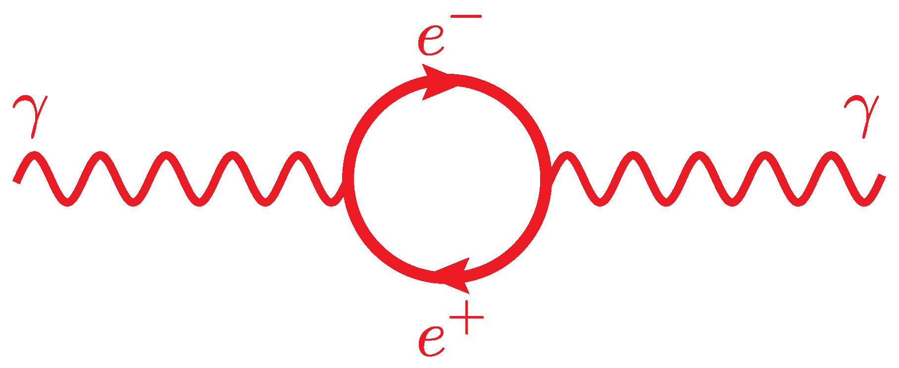
The virtual pairs discussed qualitatively in
Section 2, can be well depicted in terms of the time-honored Feynman diagrams.
Figure 2 is such a representation of vacuum polarization in the one-loop approximation. In the following we derive an expression for
using the standard technique of QED (those interested in the final result without the derivation, can go straight to Equation (
21)).
QED typically starts with a Lorentz-invariant Lagrangian density that can be written as
Here,
represents the free electromagnetic field,
describes the fermions and the interaction term reads:
where
is the external current and
is the electromagnetic four-potential with
the scalar and
the vector potentials. The Greek letters denote four-dimensional components and take the values 0 (time), 1, 2, and 3 (space). From this Lagrangian density, the wave equations for the fields describing photons and fermions are then derived. These fields are quantized to permit the creation and annihilation of particles. Charge, linear momentum, and angular momentum are conserved, so annihilation of a photon is accompanied by creation of a particle-antiparticle pair, as illustrated in
Figure 2.
An important point for the goal of this study is that the current induced in the vacuum by the four-potential,
, due to virtual pairs can be expressed as [
46]
where the Lorentz gauge is used here to simplify the equations.
Note that here, the reciprocal k-space is used. The linear response is represented by the (electron–positron) vacuum susceptibility, . Since this response must be Lorentz invariant, it has to be a function of . The condition , describing a freely propagating photon, is referred to as on-shellness in QED: a real on-shell photon verifies then . However, in collisions and other situations where one has nonpropagating fields, such as evanescent waves or near fields, will typically not be zero. The electron–positron contribution to in free space will be .
In position space, still in the Lorentz gauge, Equation (
13) becomes
If, now, one substitutes the fields,
and
, and takes into account that, for the vacuum,
and
, one obtains the gauge invariant equation,
Since it is generally true that in a dielectric,
, the
can be immediately interpreted as the vacuum current of a medium with polarization
and magnetization
, as was noted above. In Equation (
15), the vacuum magnetization current is equal d but is opposite to the polarization current, therefore leading to
.
By making use of the standard technique of Feynmann diagrams, one can show that, at lowest perturbative order, the susceptibility can be expressed as follows [
47]:
where
is the fine structure constant. The integral over the three-momentum
, represents the contribution of a photon of wave vector
exciting an electron with momentum
and a positron with momentum
. This process conserves the three-momentum
, but not the energy. As discussed above, individual pairs with quite high
do not contribute much because they are too ephemeral to polarize much. However, there are so many states with large momentum that their net contribution diverges: the cutoff,
, is introduced just to avoid that problem. If one integrates Equation (
16) over momenta and expands the result in powers of
, one obtains:
One can see that the susceptibility (
17) diverges logarithmically in the
limit. This leads to a result that seems to be physically unreasonable: the photon mass is infinite [
48], and the contribution of the virtual electron–positron pairs to the vacuum polarization diverges. However, on the other hand, this diverging vacuum susceptibility makes sense because of the screening of a point charge in a dielectric [
46]. The observable, or effective charge, positioned in the vacuum is given by
. Two arguments can be made to look at the term “squared elementary charge divided by the susceptibility”: first, this is the combination in which the quantities appear in the formula for
, and second, what counts is the interaction energy, which is a probe charge
e times the potential,
, resulting in the same combination.
In a way, for
k close to zero, the infinitely large bare charge,
, of the electron and the infinitely large vacuum susceptibility cancel each other and yield a finite effective charge [
47]. However, dividing infinities is somehow cumbersome [
4]. Alternatively, one can start with the so-called ‘regularized’ susceptibility and an observable screened charge ‘
e’. In the following, the regularized quantities are indicated by a caret:
. Far away from the point charge, for
, the regularized susceptibility has the finite observable value ‘
e’, and as one moves towards the point charge the susceptibility will approach zero, recovering the infinitely large bare charge. However, in the region of interest one deals with finite values only. The difference between the two approaches is where one hinges the
-dependence. In the first approach, one hinges the
-dependence at the bare charge, but this makes difficult to carry out any calculation. Therefore, Gottfried and Weisskopf [
4] assumed a very large but not infinitely large charge and a very small but not zero diameter of the charge distribution. The disadvantage is that as the calculation moves to an even larger charge and a correspondingly smaller diameter, the resulting susceptibility,
, changes drastically in the region far away from the bare charge in order for the increase of the charge at the origin to be compensated. On the other hand, when one hinges calculations to a region in space far enough away from the bare charge, then one deals with finite numbers and functions, and nothing has to be readjusted further away from the bare charge as the bare charge is approaching. So, here, we prefer the second approach.
The standard procedure of dealing with such a divergence is to use the experimentally observed value of the susceptibility at
and use Equation (
17) to calculate the
-dependence by subtracting two diverging terms to obtain a finite value. Thus, one expresses the susceptibility relative to its regularized on-shell value,
, i.e., the value determined experimentally,
as the relevant quantity. This is an archetypal example of a regularization of the theory.
The remaining integral can be readily performed, leading to a cumbersome analytical expression [
49,
50]. However, in the interesting limit
, Equation (
18) simplifies to
where
.
As in a standard dielectric, the linear response of the electron–positron vacuum is given by
. That is, in reciprocal
k-space:
This is quite similar to the classical electromagnetism, where
and
, but now
and
. Given the
in the numerator, Equation (
19) is a statement about the product
, not about the separate factors.
Electrons and positrons are not the only types of charged particles. To obtain the susceptibility contributed by other kinds of spin-1/2 particles, one just needs to replace
m in the previous expressions and to adjust for the electric charge,
q, hidden in
, in case
. Charged particles with spin zero also entail replacing the factor of
in the integral (
17) by
[
47]. Summing up over all elementary particle types yields the permittivity of the vacuum:
and
.
In the matter-field coupling constant,
, here, we hold
e constant and incorporate the
k-dependence into
. Since
contains all powers of
, it incorporates summation over all numbers of pairs. When restricted to an energy scale
, the sum is over all fermions of mass less than
[
51,
52,
53]. Considering
is in most ways equivalent to running of the square of effective charge in conventional QED, but the physical interpretation is different.
To obtain , one has to sum up over all particles, all of them contribute to the constant value at , summing up to 1, but for small k the running is dominated by the electron–positron vacuum because they have the largest Compton wavelength. So, in the limit of small k, one has: . In a dielectric, it is possible to have a negative induced polarization, (), when exciting above the resonance of the medium, but makes no physical sense, because in the vacuum there is no such resonance.
The dielectric properties of vacuum differ from those of a material medium in two essential points: -dependence replaces the usual -dependence and Lorentz invariance requires that . The speed is an universal constant, whereas and, thus, also the coupling constant, , runs. On the photon mass shell, , so a free photon always sees and there is no running in this case.
Finally, we argue here that the straightforward back-of-the-envelope calculation sketched in
Section 2, is consistent with QED. Actually, the loop in
Figure 2 can be thought of as a single polarizable atom with center-of-mass momentum
. If, for simplicity,
is set, the computation of the Feynman diagram involves integrals of the form
, which entails an exponential decay,
, in real space (
). Therefore, the “radius” of such a virtual atom is of order
. Alltogether, the above suggests that virtual pairs can be modelled as oscillating dipoles with frequency
and volume of order
.
Indeed, at large
and to second order in perturbation theory, Equation (
19) gives:
where a summation over all possible pairs is explicitly included. It is known [
54] that at high-momentum (or energy) scale, the coupling constant,
, in QED becomes infinity. In physical terms, charge screening can make the “renormalized” charge to adopt the finite value observed in the experiment. This is often referred to as ‘triviality’ [
48]. If
is the value of that momentum, at which
and, equivalently, at which the fine structure constant goes to infinity, usually called the Landau pole [
55], then one obtains [
27]:
While in Equation (
21) the dominant term is the one that cannot be calculated, this ambiguity is shifted in Equation (
22) to the momentum value, at which the Landau pole is located. This allows us to rewrite Equation (
21) as
Let us note that this equation is only valid for large enough
k.
Equation (
22) relates
to
. Using the experimentally determined value for
, assuming the Standard Model of QCD and summing up over all elementary particles from leptons to the W-boson with their respective charges and masses, one finds
GeV
, which is much beyond the Planck mass and is probably an unrealistically high value. Alternatively, one could assume the Minimal Super-symmetric Standard Model (MSSM), which doubles the elementary particles and thus also the sum in Equation (
22). This brings
down significantly to the value
GeV
, which is close to the momentum range, where the coupling constants are supposed to become equal. Let us note that the QED calculations referred to here are based on the one-loop approximation (see
Figure 2) and, at large momenta near the Landau pole, multiple loop contributions will be significant. In that sense the concept of the Landau momentum (or Landau pole) based on the one-loop approximation has limited value. Nevertheless, it well demonstrates the concept.
If one compares the terms in the sum (
22) with the ones in Equation (
9), one by one, one finds that the two equations, provided that
To fulfill Equation (
24) one would have to give up the assumption that the ratio of the Compton wavelength cubed and the volume occupied by a single virtual pair is independent of the type of elementary particle. This may not be reasonable. However, instead of doing the detailed evaluation of the sum in Equation (
22), we can perform here some estimations: the masses
differ by a factor
, but this factor is diminished by the logarithmic function. As a result, the logarithmic term is almost constant for large enough cutoff
and, to some approximation, can be taken out of the sum. The term
varies only little when assuming the Standard Model and its average is 144. If, as an approximation, all logarithmic terms in the sum are replaced by 144, then one obtains the condition that
So, one gets the correct value by adjusting the volume per virtual pair in the model discussed here to a reasonable value close to the Compton wavelength cubed, or by choosing the right value for the Landau pole, .
Let us stress that in the model here, no divergence appears, the only uncertainty is associated with the volume occupied by each virtual pair. The position variance of the harmonic oscillator ground state wave function gives a crude value for the volume per pair in the right ball park, but it does not give a precise value. There is a different way to estimate this volume in momentum space: in analogy to the derivation of Planck’s blackbody radiation formula, one can calculate the number of modes (i. e., standing waves) of the particle’s de Broglie wave pattern in a given larger volume, integrate over momentum (inversely proportional to the de Broglie wavelength) and divide the larger volume by the the number of modes obtained. This then determines the volume per mode or per particle-antiparticle pair. However, this integral diverges and one would obtain
. A crude cure would be to introduce a relativistic cutoff which will also give a volume per pair of the order of the particle Compton wavelength cubed. Staying in configuration space as opposed to momentum space, one seems to avoid this divergence, as suggested by Fried and Gabellini [
56], who discuss the advantage of performing QED calculation in configuration space. It remains to find if a more precise value for the volume per pair can be derived using a configuration-space description.
The standard approach in QED is to use plane waves to describe the relative motion of the virtual pairs. In the center of mass reference frame, if the electron has momentum , then the positron has momentum . However, the uncertainty principle requires that the lifetime of the pair is quite short, so the distance travelled d is comparably small. The plane-wave basis seems not suited well enough in order to describe this situation: convergence is quite poor, and the divergences arise. What would be needed is a basis whose ground and first few excited states are of comparable size to d. The merit of the oscillator model is to provide a suitable basis for description of the relative motion in these short lived states.


