Diffusion in Phase Space as a Tool to Assess Variability of Vertical Centre-of-Mass Motion during Long-Range Walking

 ,
,  , , and
Abstract
:1. Introduction
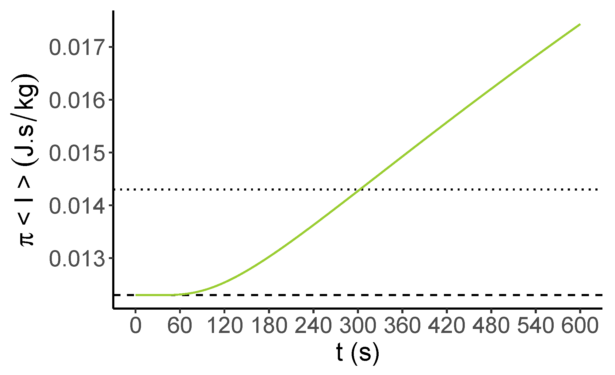
2. Diffusion in Phase Space
2.1. Generalities
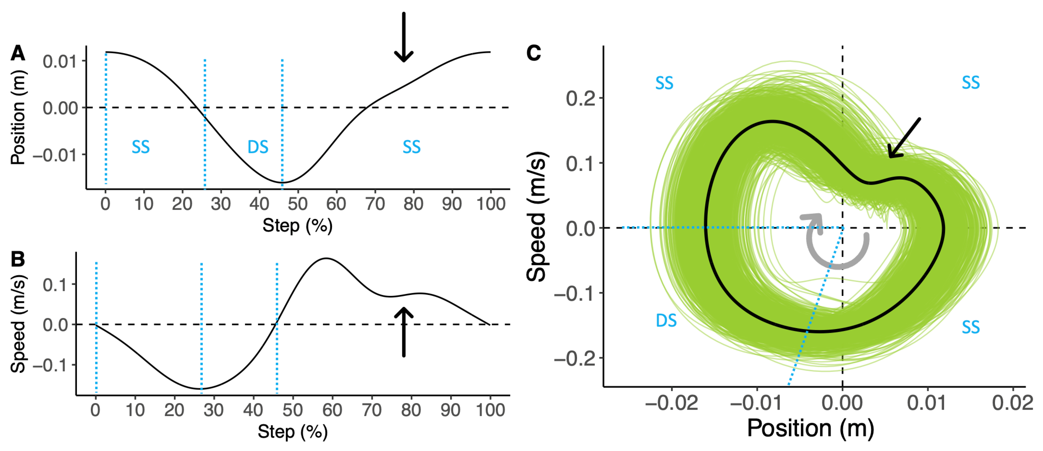
2.2. Application to Human Walking
3. Experimental Setup
3.1. Protocol
3.2. Data Processing
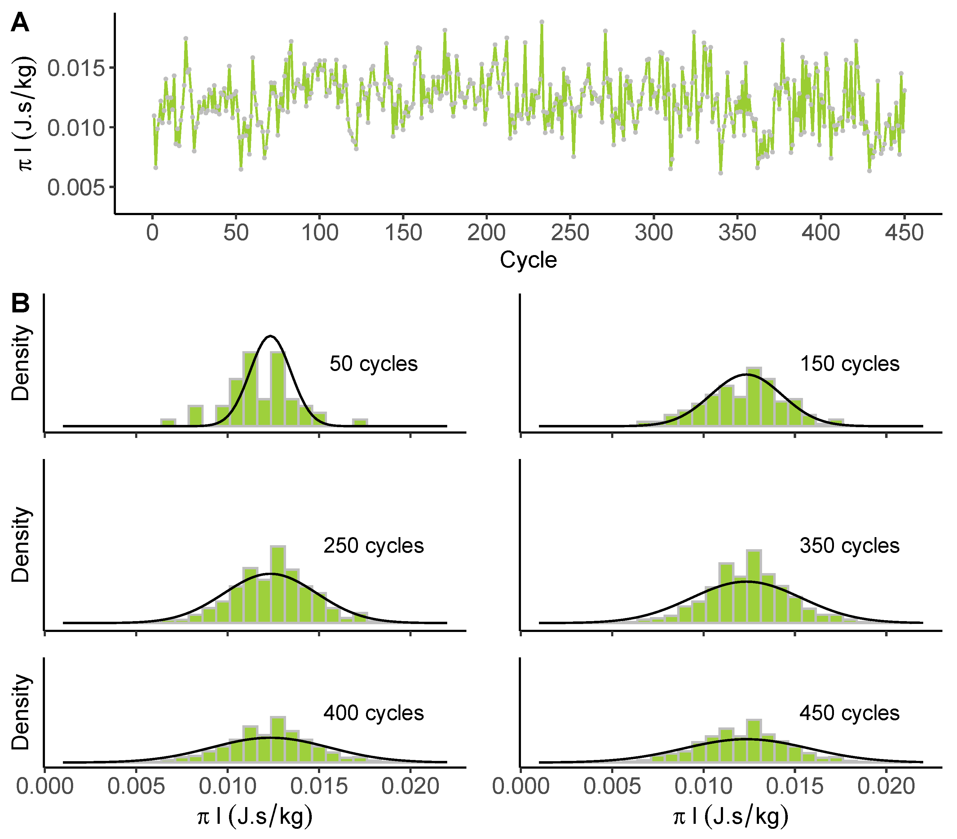
4. Results
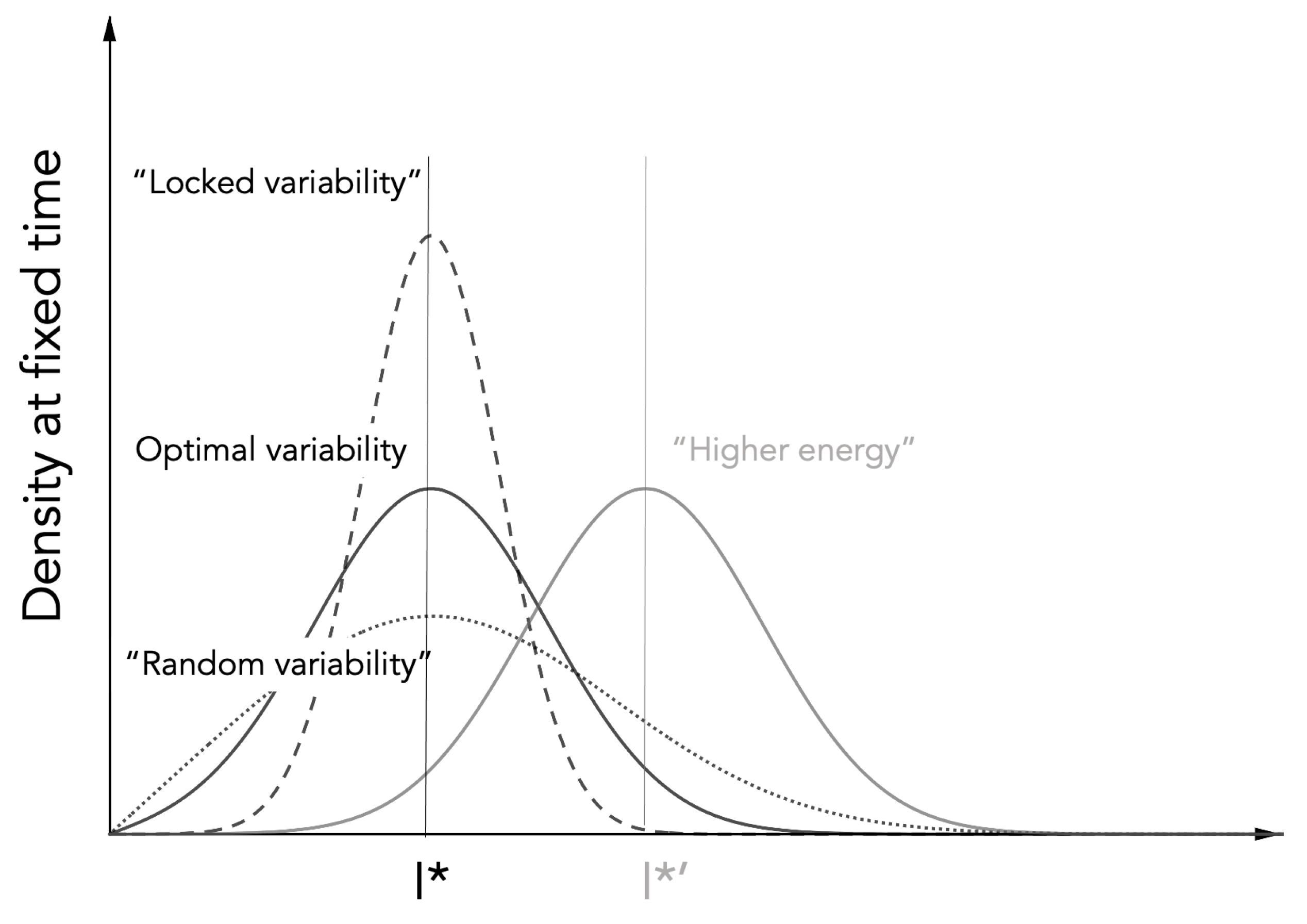
5. Discussion
Author Contributions
Funding
Institutional Review Board Statement
Informed Consent Statement
Data Availability Statement
Acknowledgments
Conflicts of Interest
References
- Landau, L.; Lifchitz, E. Physique Théorique, Tome 1: Mécanique; Éditions MIR: Moscow, Russia, 1988. [Google Scholar]
- Kolmogorov, A.N. On conservation of conditionally periodic motions for a small change in Hamilton’s function. Dokl. Akad. Nauk SSSR 1954, 98, 527–530. (In Russian) [Google Scholar]
- Kolmogorov, A.N. Preservation of conditionally periodic movements with small change in the Hamilton function. In Stochastic Behavior in Classical and Quantum Hamiltonian Systems; Casati, G., Ford, J., Eds.; Springer: Berlin/Heidelberg, Germany, 1979; pp. 51–56. [Google Scholar] [CrossRef]
- Arnol’d, V.I. Proof of a theorem of A.N. Kolmogorov on the invariance of quadi-periodic motions under small perturbations of the hamiltonian. Russ. Math. Surv. 1963, 18, 9–36. [Google Scholar] [CrossRef]
- Möser, J. On invariant curves of area-preserving mappings of an annulus. Nachr. Akad. Wiss. Göttingen II Math.-Phys. Kl. 1962, 1962, 1–20. [Google Scholar]
- Scott Dumas, H. The KAM Story: A Friendly Introduction to the Content, History, and Significance of Classical Kolmogorov-Arnold-Moser Theory; World Scientific: Hackensack, NJ, USA, 2014. [Google Scholar] [CrossRef]
- Nekhoroshev, N. Behavior of Hamiltonian systems close to integrable. Funct. Anal. Its Appl. 1971, 5, 338–339. [Google Scholar] [CrossRef]
- Nekhoroshev, N. An exponential estimate of the time of stability of nearly-integrable Hamiltonian systems. Russ. Math. Surv. 1977, 32, 1. [Google Scholar] [CrossRef]
- Henrard, J. The adiabatic invariant in classical mechanics. In Dynamics Reported.; Kirchgraber, U., Walther, H.O., Eds.; Springer: Berlin/Heidelberg, Germany, 1993; Volume 2, pp. 117–235. [Google Scholar] [CrossRef]
- Jose, J.V.; Saletan, E.J. Classical Dynamics: A Contemporary Approach; Cambridge University Press: Cambridge, UK, 1998. [Google Scholar] [CrossRef]
- Khas’minskii, R.Z. On Stochastic processes defined by differential equations with a small parameter. Theory Probab. Its Appl. 1966, 11, 211–228. [Google Scholar] [CrossRef]
- Cogburn, R.; Ellison, J.A. A stochastic theory of adiabatic invariance. Commun. Math. Phys. 1992, 149, 97–126. [Google Scholar] [CrossRef]
- Bazzani, A.; Siboni, S.; Turchetti, G.; Vaienti, S. A model of modulated diffusion. I. Analytical results. J. Stat. Phys. 1994, 76, 929–967. [Google Scholar] [CrossRef]
- Bazzani, A.; Siboni, S.; Turchetti, G. Diffusion in stochastically and periodically modulated Hamiltonian systems. AIP Conf. Proc. 1995, 344, 68–77. [Google Scholar] [CrossRef]
- Bazzani, A.; Beccaceci, L. Diffusion in Hamiltonian systems driven by harmonic noise. J. Phys. A Math. Gen. 1998, 31, 5843–5854. [Google Scholar] [CrossRef]
- Kominis, Y.; Ram, A.K.; Hizanidis, K. Kinetic Theory for Distribution Functions of Wave-Particle Interactions in Plasmas. Phys. Rev. Lett. 2010, 104, 235001. [Google Scholar] [CrossRef]
- Degond, P.; Herda, M.; Mirrahimi, S. A Fokker-Planck approach to the study of robustness in gene expression. Math. Biosci. Eng. 2020, 17, 6459–6486. [Google Scholar] [CrossRef]
- Hausdorff, J.M.; Peng, C.K.; Ladin, Z.; Wei, J.Y.; Goldberger, A.L. Is walking a random walk? Evidence for long-range correlations in stride interval of human gait. J. Appl. Physiol. 1995, 78, 349–358. [Google Scholar] [CrossRef]
- Hausdorff, J.M.; Mitchell, S.L.; Firtion, R.; Peng, C.K.; Cudkowicz, M.E.; Wei, J.Y.; Goldberger, A.L. Altered fractal dynamics of gait: Reduced stride-interval correlations with aging and Huntington’s disease. J. Appl. Physiol. 1997, 82, 262–269. [Google Scholar] [CrossRef]
- Stergiou, N.A. Nonlinear Analysis for Human Movement Variability; CRC Press/Taylor & Francis Group: Boca Raton, FL, USA, 2016; Volume 7. [Google Scholar] [CrossRef]
- Ravi, D.K.; Marmelat, V.; Taylor, W.R.; Newell, K.M.; Stergiou, N.; Singh, N.B. Assessing the temporal organization of walking variability: A systematic review and consensus guidelines on detrended fluctuation analysis. Front. Physiol. 2020, 11, 562. [Google Scholar] [CrossRef]
- Risken, H. The Fokker-Planck Equation: Methods of Solution and Applications Second Edition; Springer: Berlin/Heidelberg, Germany, 1996. [Google Scholar] [CrossRef]
- Fa, K.S. Exact solution of the Fokker-Planck equation for a broad class of diffusion coefficients. Phys. Rev. E 2005, 72, 020101. [Google Scholar] [CrossRef] [Green Version]
- Lin, W.T.; Ho, C.L. Similarity solutions of the Fokker–Planck equation with time-dependent coefficients. Ann. Phys. 2012, 327, 386–397. [Google Scholar] [CrossRef]
- Cavagna, G.; Thys, H.; Zamboni, A. The sources of external work in level walking and running. J. Physiol. 1976, 262, 639–657. [Google Scholar] [CrossRef]
- Cavagna, G.A.; Legramandi, M.A. The phase shift between potential and kinetic energy in human walking. J. Exp. Biol. 2020, 223, jeb232645. [Google Scholar] [CrossRef]
- Whittington, B.R.; Thelen, D.G. A simple mass-spring model with roller feet can induce the ground reactions observed in human walking. J. Biomech. Eng. 2008, 131, 011013. [Google Scholar] [CrossRef]
- Brizard, A.J. Jacobi zeta function and action-angle coordinates for the pendulum. Commun. Nonlinear Sci. Numer. Simul. 2013, 18, 511–518. [Google Scholar] [CrossRef]
- Buisseret, F.; Dehouck, V.; Boulanger, N.; Henry, G.; Piccinin, F.; White, O.; Dierick, F. Adiabatic Invariant of Center-of-Mass Motion during Walking as a Dynamical Stability Constraint on Stride Interval Variability and Predictability. Biology 2022, 11, 1334. [Google Scholar] [CrossRef] [PubMed]
- Sturges, H.A. The Choice of a Class Interval. J. Am. Stat. Assoc. 1926, 21, 65–66. [Google Scholar] [CrossRef]
- The R Project for Statistical Computing. Available online: https://www.r-project.org (accessed on 10 January 2023).
- Broscheid, K.-C.; Dettmers, C.; Vieten, M. Is the Limit-Cycle-Attractor an (almost) invariable characteristic in human walking? Gait Posture 2018, 63, 242–247. [Google Scholar] [CrossRef]
- Raffalt, P.; Kent, J.; Wurdeman, S.; Stergiou, N. To walk or to run—A question of movement attractor stability. J. Exp. Biol. 2020, 223, jeb224113. [Google Scholar] [CrossRef]
- Adamczyk, P.G.; Kuo, A.D. Redirection of center-of-mass velocity during the step-to-step transition of human walking. J. Exp. Biol. 2009, 212, 2668–2678. [Google Scholar] [CrossRef] [Green Version]
- White, O.; Gaveau, J.; Bringoux, L.; Crevecoeur, F. The gravitational imprint on sensorimotor planning and control. J. Neurophysiol. 2020, 124, 4–19. [Google Scholar] [CrossRef]
- Goldberger, A.L.; Amaral, L.A.N.; Hausdorff, J.M.; Ivanov, P.C.; Peng, C.K.; Stanley, H.E. Fractal dynamics in physiology: Alterations with disease and aging. Proc. Natl. Acad. Sci. USA 2002, 99, 2466–2472. [Google Scholar] [CrossRef] [PubMed]
- Stergiou, N.; Harbourne, R.; Cavanaugh, J. Optimal movement variability: A new theoretical perspective for neurologic physical therapy. J. Neurol. Phys. Ther. 2006, 30, 120–129. [Google Scholar] [CrossRef]
- van Emmerik, R.E.; Ducharme, S.W.; Amado, A.C.; Hamill, J. Comparing dynamical systems concepts and techniques for biomechanical analysis. J. Sport Health Sci. 2016, 5, 3–13. [Google Scholar] [CrossRef]
- Moon, Y.; Sung, J.; An, R.; Hernandez, M.E.; Sosnoff, J.J. Gait variability in people with neurological disorders: A systematic review and meta-analysis. Hum. Mov. Sci. 2016, 47, 197–208. [Google Scholar] [CrossRef] [PubMed]
- Hausdorff, J.M.; Zemany, L.; Peng, C.K.; Goldberger, A.L. Maturation of gait dynamics: Stride-to-stride variability and its temporal organization in children. J. Appl. Physiol. 1999, 86, 1040–1047. [Google Scholar] [CrossRef] [PubMed]
- Dizio, P.; Lackner, J.R. Motor adaptation to Coriolis force perturbations of reaching movements: Endpoint but not trajectory adaptation transfers to the nonexposed arm. J. Neurophysiol. 1995, 74, 1787–1792. [Google Scholar] [CrossRef]
- Criscimagna-Hemminger, S.E.; Donchin, O.; Gazzaniga, M.S.; Shadmehr, R. Learned dynamics of reaching movements generalize from dominant to nondominant arm. J. Neurophysiol. 2003, 89, 168–176. [Google Scholar] [CrossRef]
- Sarwary, A.M.E.; Stegeman, D.F.; Selen, L.P.J.; Medendorp, W.P. Generalization and transfer of contextual cues in motor learning. J. Neurophysiol. 2015, 114, 1565–1576. [Google Scholar] [CrossRef]
- Shadmehr, R.; Mussa-Ivaldi, F.A. Adaptive representation of dynamics during learning of a motor task. J. Neurosci. 1994, 14, 3208–3224. [Google Scholar] [CrossRef]
- Thoroughman, K.A.; Shadmehr, R. Learning of action through adaptive combination of motor primitives. Nature 2000, 407, 742–747. [Google Scholar] [CrossRef]


| Population Feature | Median, Interval |
|---|---|
| Participants (n) | 25 |
| Age (years) | 23 [20–23] |
| Mass (kg) | 65.0 [58.8–73.4] |
| Height (cm) | 169 [164–176] |
| Walking speed (km/h) | 3.9 [3.5–4.2] |
| Sex (men/women) | 9/16 |
| Gait cycles | 532 [513–552] |
| Parameter | Fit Value | p-Value |
|---|---|---|
| D (10 m2/s) | 11.618 [6.024–37.712] | <0.001 |
| (J·s/kg) | 0.0123 [0.0061–0.0178] | <0.001 |
| (%) | 100 [98.6–100] |
Disclaimer/Publisher’s Note: The statements, opinions and data contained in all publications are solely those of the individual author(s) and contributor(s) and not of MDPI and/or the editor(s). MDPI and/or the editor(s) disclaim responsibility for any injury to people or property resulting from any ideas, methods, instructions or products referred to in the content. |
© 2023 by the authors. Licensee MDPI, Basel, Switzerland. This article is an open access article distributed under the terms and conditions of the Creative Commons Attribution (CC BY) license (https://creativecommons.org/licenses/by/4.0/).
Share and Cite
Boulanger, N.; Buisseret, F.; Dehouck, V.; Dierick, F.; White, O. Diffusion in Phase Space as a Tool to Assess Variability of Vertical Centre-of-Mass Motion during Long-Range Walking. Physics 2023, 5, 168-178. https://doi.org/10.3390/physics5010013
Boulanger N, Buisseret F, Dehouck V, Dierick F, White O. Diffusion in Phase Space as a Tool to Assess Variability of Vertical Centre-of-Mass Motion during Long-Range Walking. Physics. 2023; 5(1):168-178. https://doi.org/10.3390/physics5010013
Chicago/Turabian StyleBoulanger, Nicolas, Fabien Buisseret, Victor Dehouck, Frédéric Dierick, and Olivier White. 2023. "Diffusion in Phase Space as a Tool to Assess Variability of Vertical Centre-of-Mass Motion during Long-Range Walking" Physics 5, no. 1: 168-178. https://doi.org/10.3390/physics5010013