
An Artificial Neural Network for Predicting Groundnut Yield Using Climatic Data

 ,
,  ,
,  , and
, and 
Abstract
:1. Introduction
2. Materials and Methods
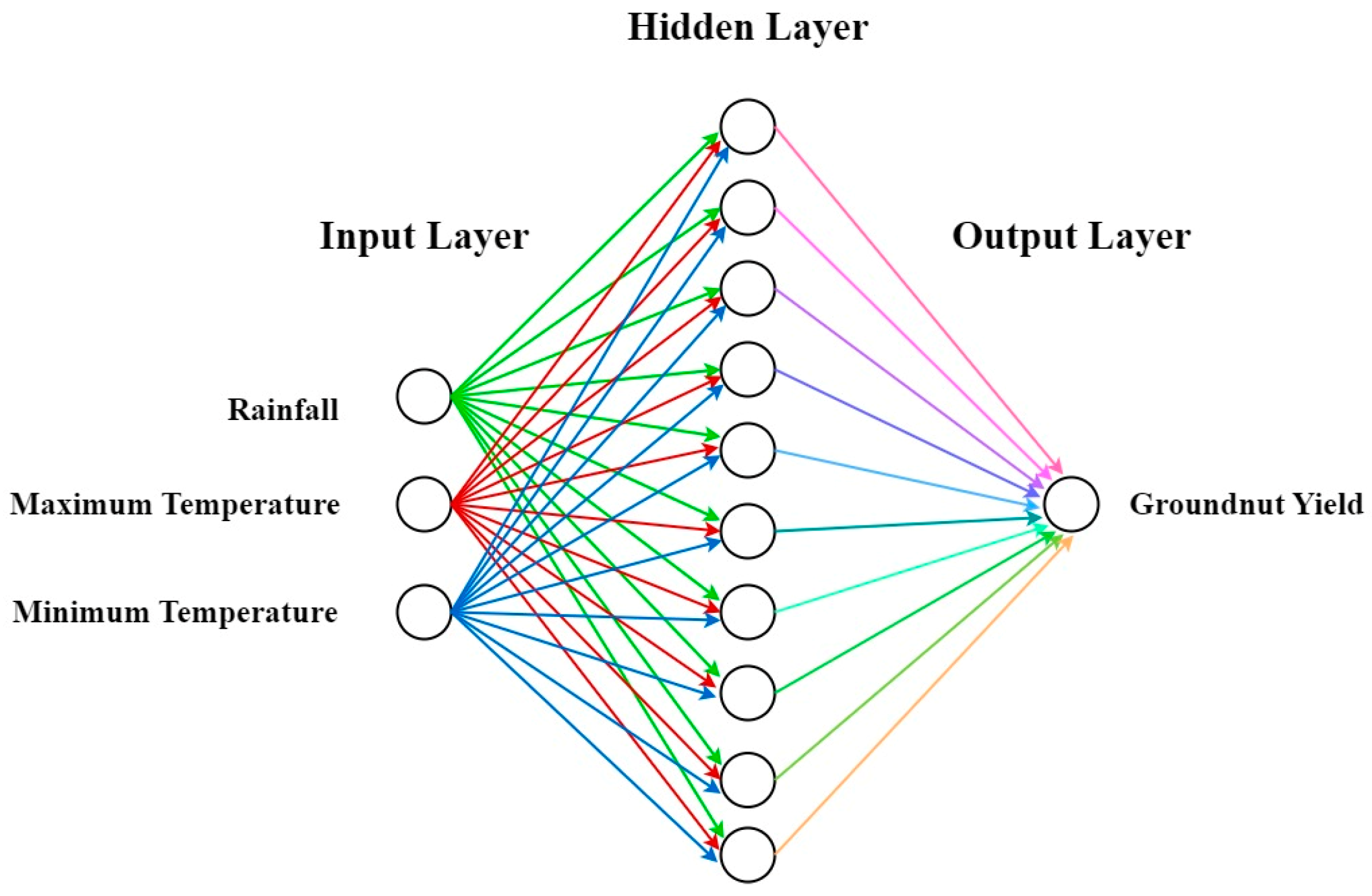
2.1. Artificial Neural Networks and Their Training Algorithms
2.1.1. Levenberg–Marquardt Algorithm
2.1.2. Bayesian Regularization Algorithm
2.1.3. Scaled Conjugate Gradient Algorithm
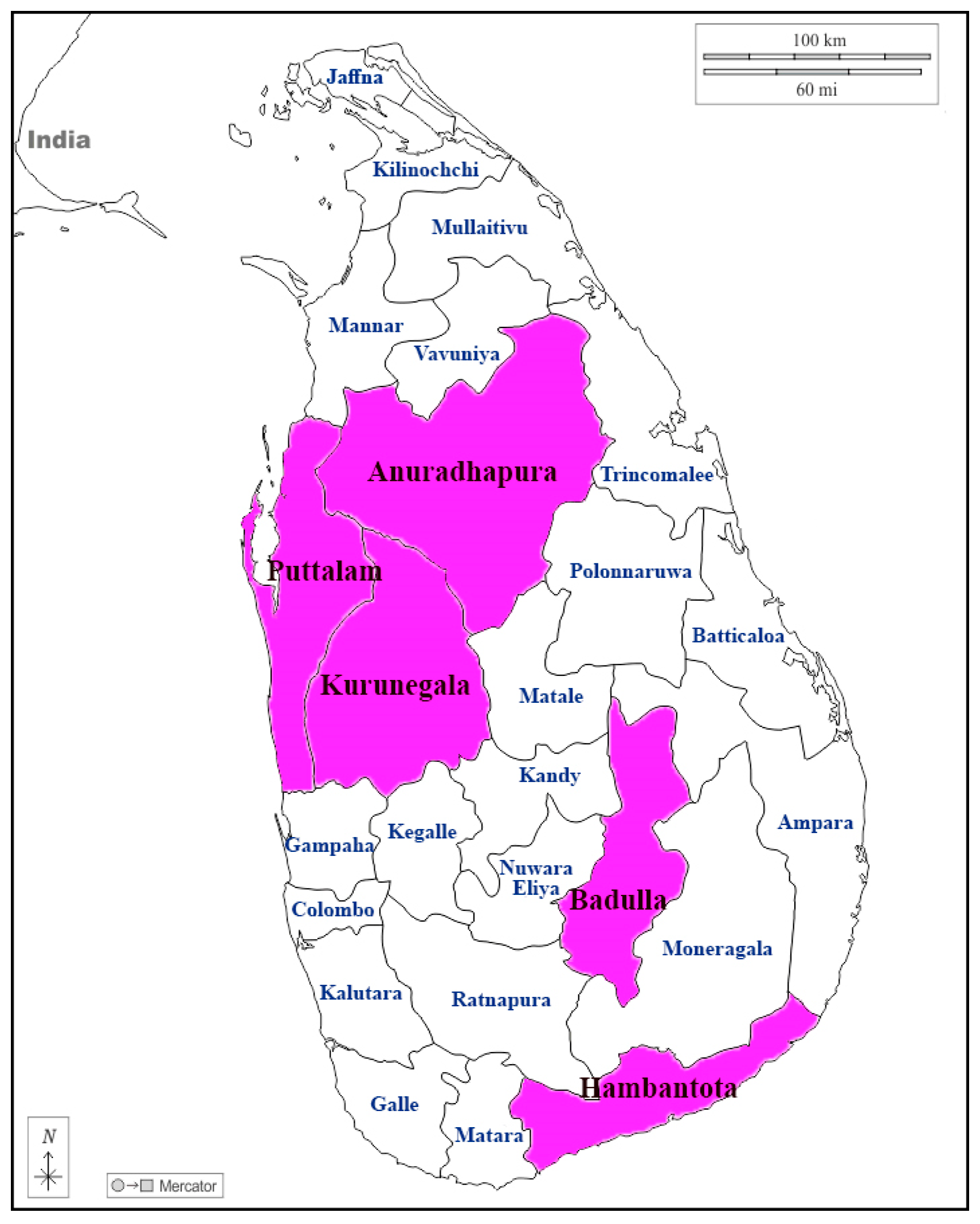
2.2. Study Area and Data
2.3. Problem Formulation
2.4. Model Accuracy Evaluation
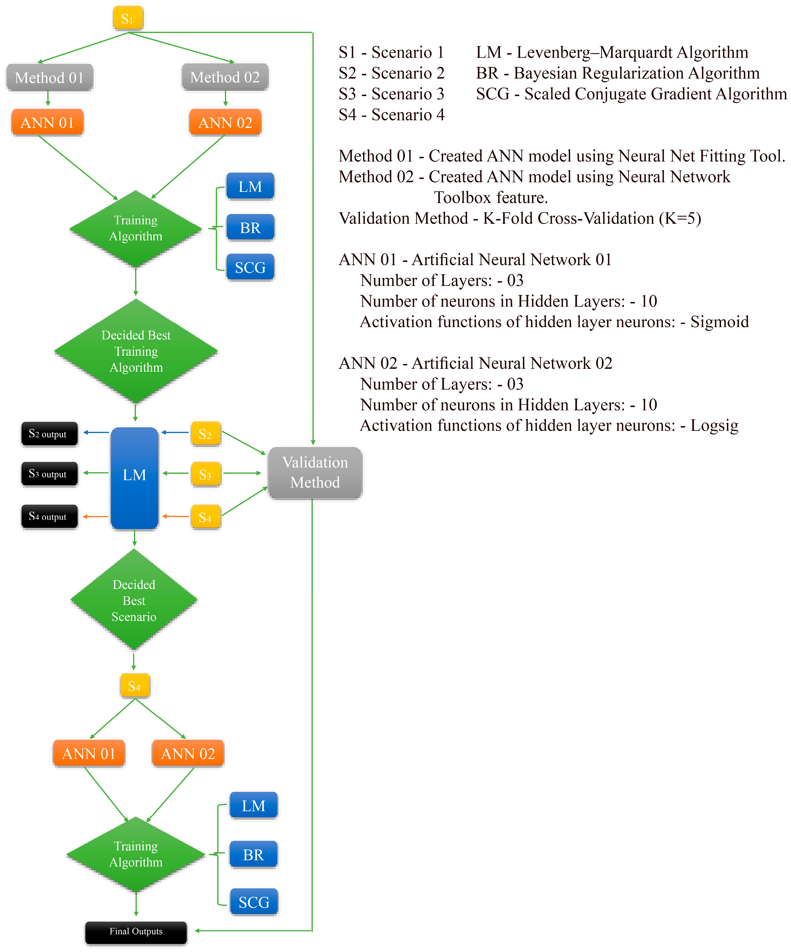
2.5. Overall Methodology
3. Results
3.1. Results Obtained Using Method 1
3.2. Results Obtained Using Method 2
3.3. Results Obtained Using K-Fold Cross Validation Method
4. Discussion
4.1. Evaluating the Climatic Data with Groundnut Yield using Method 1
4.2. Evaluating the Climatic Data with Groundnut Yield using Method 2
4.3. Validation of the Climatic Data with Groundnut Yield using the K-Fold Cross-Validation Method
4.4. Previous Similar Studies
5. Conclusions
6. Suggestions and Future Research
Author Contributions
Funding
Data Availability Statement
Conflicts of Interest
References
- Janila, P.; Nigam, S.N.; Pandey, M.K.; Nagesh, P.; Varshney, R.K. Groundnut improvement: Use of genetic and genomic tools. Front. Plant Sci. 2013, 4, 23. [Google Scholar] [CrossRef] [PubMed]
- Belayneh, D.B.; Chondie, Y.G. Participatory variety selection of groundnut (Arachis hypogaea L.) in Taricha Zuriya district of Dawuro Zone, southern Ethiopia. Heliyon 2022, 8, e09011. [Google Scholar] [CrossRef] [PubMed]
- Alagirisamy, M. Groundnut. Breed. Oilseed Crops Sustain. Prod. 2016, 89–134. [Google Scholar] [CrossRef]
- United States Department of Agriculture (USDA). Available online: https://ipad.fas.usda.gov/cropexplorer/cropview/commodityView.aspx?cropid=2221000&sel_year=2022&rankby=Production (accessed on 25 June 2023).
- Ezihe, J.A.C.; Agbugba, I.K.; Idang, C. Effect of climatic change and variability on groundnut (Arachis hypogea L.) production in Nigeria. Bulg. J. Agric. Sci. 2017, 23, 906–914. [Google Scholar]
- Janani, H.K.; Abeysiriwardana, H.D.; Rathnayake, U.; Sarukkalige, R. Water Footprint Assessment for Irrigated Paddy Cultivation in Walawe Irrigation Scheme, Sri Lanka. Hydrology 2022, 9, 210. [Google Scholar] [CrossRef]
- Thilini, S.; Pradheeban, L.; Nishanthan, K. Effect of Different Time of Earthing Up on Growth and Yield Performances of Groundnut (Arachis hypogea L.) Varieties. Available online: http://repo.lib.jfn.ac.lk/ujrr/handle/123456789/1581 (accessed on 6 July 2023).
- Jeewani, D.C.; Amarasinghe, Y.P.J.; Wijesinghe, G.; Kumara, R.W.P. Screening exotic groundnut (Arachis hypogaea L.) lines for introducing as a small-seeded variety (ANKGN4/Tiny) in Sri Lanka. Trop. Agric. Res. Ext. 2021, 24, 330. [Google Scholar] [CrossRef]
- Department of Census and Statistics Ministry of Finance. Available online: http://www.statistics.gov.lk/Publication/PocketBook (accessed on 26 June 2023).
- Adisa, O.M.; Botai, J.O.; Adeola, A.M.; Hassen, A.; Botai, C.M.; Darkey, D.; Tesfamariam, E. Application of Artificial Neural Network for Predicting Maize Production in South Africa. Sustainability 2019, 11, 1145. [Google Scholar] [CrossRef]
- Gopal, P.M.; Bhargavi, R. A novel approach for efficient crop yield prediction. Comput. Electron. Agric. 2019, 165, 104968. [Google Scholar] [CrossRef]
- Amaratunga, V.; Wickramasinghe, L.; Perera, A.; Jayasinghe, J.; Rathnayake, U. Artificial Neural Network to Estimate the Paddy Yield Prediction Using Climatic Data. Math. Probl. Eng. 2020, 2020, 8627824. [Google Scholar] [CrossRef]
- Kho, S.J.; Manickam, S.; Malek, S.; Mosleh, M.; Dhillon, S.K. Automated plant identification using artificial neural network and support vector machine. Front. Life Sci. 2017, 10, 98–107. [Google Scholar] [CrossRef]
- Ranjan, M.; Rajiv, W.M.; Joshi, N.; Ingole, A. Detection and classification of leaf disease using artificial neural network. Int. J. Tech. Res. Appl. 2015, 3, 331–333. [Google Scholar]
- Bargoti, S.; Underwood, J.P. Image segmentation for fruit detection and yield estimation in apple orchards. J. Field Robot. 2017, 34, 1039–1060. [Google Scholar] [CrossRef]
- Patil, P.U.; Lande, S.B.; Nagalkar, V.J.; Nikam, S.B.; Wakchaure, G. Grading and sorting technique of dragon fruits using machine learning algorithms. J. Agric. Food Res. 2021, 4, 100118. [Google Scholar] [CrossRef]
- Bhimani, P.C.; Anand Agricultural University; Gundaniya, H.V.; Darji, V.B. Forecasting of Groundnut Yield Using Meteorological Variables. Gujarat J. Ext. Educ. 2022, 34, 139–142. [Google Scholar] [CrossRef]
- Biswas, M.R.; Alzubaidi, M.S.; Shah, U.; Abd-Alrazaq, A.A.; Shah, Z. A Scoping Review to Find out Worldwide COVID-19 Vaccine Hesitancy and Its Underlying Determinants. Vaccines 2022, 9, 1243. [Google Scholar] [CrossRef]
- Aravind, K.S.; Vashisth, A.; Krishanan, P.; Das, B. Wheat yield prediction based on weather parameters using multiple linear, neural network and penalised regression models. J. Agrometeorol. 2022, 24, 18–25. [Google Scholar] [CrossRef]
- Aubakirova, G.; Ivel, V.; Gerassimova, Y.; Moldakhmetov, S.; Petrov, P. Application of artificial neural network for wheat yield forecasting. Eastern-European J. Enterp. Technol. 2022, 3, 31–39. [Google Scholar] [CrossRef]
- Rojas, R. Neural Networks: A Systematic Introduction, 1st ed.; Springer: New York, NY, USA, 1996. [Google Scholar] [CrossRef]
- Morales, A.; Villalobos, F.J. Using machine learning for crop yield prediction in the past or the future. Front. Plant Sci. 2023, 14, 1128388. [Google Scholar] [CrossRef]
- Sapna, S. Backpropagation Learning Algorithm Based on Levenberg Marquardt Algorithm. Comput. Sci. Inf. Technol. 2012, 2, 393–398. [Google Scholar] [CrossRef]
- Unke, O.T.; Chmiela, S.; Sauceda, H.E.; Gastegger, M.; Poltavsky, I.; Schütt, K.T.; Tkatchenko, A.; Müller, K.-R. Machine Learning Force Fields. Chem. Rev. 2021, 121, 10142–10186. [Google Scholar] [CrossRef]
- Cetişli, B.; Barkana, A. Speeding up the scaled conjugate gradient algorithm and its application in neuro-fuzzy classifier training. Soft Comput. 2009, 14, 365–378. [Google Scholar] [CrossRef]
- Aghelpour, P.; Bagheri-Khalili, Z.; Varshavian, V.; Mohammadi, B. Evaluating Three Supervised Machine Learning Algorithms (LM, BR, and SCG) for Daily Pan Evaporation Estimation in a Semi-Arid Region. Water 2022, 14, 3435. [Google Scholar] [CrossRef]
- Heng, S.Y.; Ridwan, W.M.; Kumar, P.; Ahmed, A.N.; Fai, C.M.; Birima, A.H.; El-Shafie, A. Artificial neural network model with different backpropagation algorithms and meteorological data for solar radiation prediction. Sci. Rep. 2022, 12, 10457. [Google Scholar] [CrossRef] [PubMed]
- Rahman, A.; Kang, S.; Nagabhatla, N.; Macnee, R. Impacts of temperature and rainfall variation on rice productivity in major ecosystems of Bangladesh. Agric. Food Secur. 2017, 6, 10. [Google Scholar] [CrossRef]
- Chemura, A.; Schauberger, B.; Gornott, C. Impacts of climate change on agro-climatic suitability of major food crops in Ghana. PLoS ONE 2020, 15, e0229881. [Google Scholar] [CrossRef]
- Semenov, M.A.; Shewry, P.R. Modelling predicts that heat stress, not drought, will increase vulnerability of wheat in Europe. Sci. Rep. 2011, 1, 66. [Google Scholar] [CrossRef]
- Zhao, C.; Liu, B.; Piao, S.; Wang, X.; Lobell, D.B.; Huang, Y.; Huang, M.T.; Yao, Y.T.; Bassu, S.; Ciais, P.; et al. Temperature increase reduces global yields of major crops in four independent estimates. Proc. Natl. Acad. Sci. USA 2017, 114, 9326–9331. [Google Scholar] [CrossRef]
- Lopes, M.S. Will temperature and rainfall changes prevent yield progress in Europe? Food Energy Secur. 2022, 11, e372. [Google Scholar] [CrossRef]
- Ansari, H.; Zarei, M.; Sabbaghi, S.; Keshavarz, P. A new comprehensive model for relative viscosity of various nanofluids using feed-forward back-propagation MLP neural networks. Int. Commun. Heat Mass Transf. 2018, 91, 158–164. [Google Scholar] [CrossRef]
- Du, Y.-C.; Stephanus, A. Levenberg-Marquardt Neural Network Algorithm for Degree of Arteriovenous Fistula Stenosis Classification Using a Dual Optical Photoplethysmography Sensor. Sensors 2018, 18, 2322. [Google Scholar] [CrossRef]
- Berglund, E. Novel Hessian Approximations in Optimization Algorithms. Ph.D. Thesis, KTH Royal Institute of Technology, Stockholm, Sweden, 2022. [Google Scholar]
- Perera, A.; Rathnayake, U. Rainfall and Atmospheric Temperature against the Other Climatic Factors: A Case Study from Colombo, Sri Lanka. Math. Probl. Eng. 2019, 2019, 5692753. [Google Scholar] [CrossRef]
- Ramadasan, D.; Chevaldonné, M.; Chateau, T. LMA: A generic and efficient implementation of the Levenberg-Marquardt Algorithm. Softw. Pract. Exp. 2017, 47, 1707–1727. [Google Scholar] [CrossRef]
- Chaudhary, N.; Younus, O.I.; Alves, L.N.; Ghassemlooy, Z.; Zvanovec, S. The Usage of ANN for Regression Analysis in Visible Light Positioning Systems. Sensors 2022, 22, 2879. [Google Scholar] [CrossRef] [PubMed]
- Bishop, C.M. Neural Network for Pattern Recognition; Department of Computer Science and Applied Mathematics, Aston University: Birmingham, UK, 1995. [Google Scholar]
- Murphy, M.D.; O’Mahony, M.J.; Shalloo, L.; French, P.; Upton, J. Comparison of modelling techniques for milk-production forecasting. J. Dairy Sci. 2014, 97, 3352–3363. [Google Scholar] [CrossRef]
- Mammadli, S. Financial time series prediction using artificial neural network based on Levenberg-Marquardt algorithm. Procedia Comput. Sci. 2017, 120, 602–607. [Google Scholar] [CrossRef]
- Zhang, X.; Liu, H.; Wang, X.; Dong, L.; Wu, Q.; Mohan, R. Speed and convergence properties of gradient algorithms for optimization of IMRT. Med. Phys. 2004, 31, 1141–1152. [Google Scholar] [CrossRef]
- Selvamuthu, D.; Kumar, V.; Mishra, A. Indian stock market prediction using artificial neural networks on tick data. Financ. Innov. 2019, 5, 16. [Google Scholar] [CrossRef]
- Shine, P.; Scully, T.; Upton, J. Murphy Multiple linear regression modelling of on-farm direct water and electricity consumption on pasture based dairy farms. Comput. Electron. Agric. 2018, 148, 337–346. [Google Scholar] [CrossRef]
- Murphy, M.D.; O’Sullivan, P.D.; da Graça, G.C.; O’Donovan, A. Development, Calibration and Validation of an Internal Air Temperature Model for a Naturally Ventilated Nearly Zero Energy Building: Comparison of Model Types and Calibration Methods. Energies 2021, 14, 871. [Google Scholar] [CrossRef]
- Prusty, S.; Patnaik, S.; Dash, S.K. SKCV: Stratified K-fold cross-validation on ML classifiers for predicting cervical cancer. Front. Nanotechnol. 2022, 4, 972421. [Google Scholar] [CrossRef]
- Legates, D.R.; McCabe, G.J.J. Evaluating the use of “goodness-of-fit” Measures in hydrologic and hydroclimatic model validation. Water Resour. Res. 1999, 35, 233–241. [Google Scholar] [CrossRef]
- Nezhad, E.F.; Ghalhari, G.F.; Bayatani, F. Forecasting Maximum Seasonal Temperature Using Artificial Neural Networks “Tehran Case Study”. Asia-Pacific J. Atmos. Sci. 2019, 55, 145–153. [Google Scholar] [CrossRef]
- Peters, S.O.; Sinecen, M.; Gallagher, G.R.; Pebworth, L.A.; Jacob, S.; Hatfield, J.S.; Kizilkaya, K. Comparison of linear model and artificial neural network using antler beam diameter and length of white-tailed deer (Odocoileus virginianus) dataset. PLoS ONE 2019, 14, e0212545. [Google Scholar] [CrossRef]
- Aneja, S.; Sharma, A.; Gupta, R.; Yoo, D.-Y. Bayesian Regularized Artificial Neural Network Model to Predict Strength Characteristics of Fly-Ash and Bottom-Ash Based Geopolymer Concrete. Materials 2021, 14, 1729. [Google Scholar] [CrossRef] [PubMed]
- Gavin, H.P. The Levenberg-Marquardt Algorithm for Nonlinear Least Squares Curve-Fitting Problems; Duke University: Durham, NC, USA, 2019. [Google Scholar]
- Yadav, A.; Chithaluru, P.; Singh, A.; Joshi, D.; Elkamchouchi, D.H.; Pérez-Oleaga, C.M.; Anand, D. An Enhanced Feed-Forward Back Propagation Levenberg–Marquardt Algorithm for Suspended Sediment Yield Modeling. Water 2022, 14, 3714. [Google Scholar] [CrossRef]
- Finsterle, S.; Kowalsky, M.B. A truncated Levenberg–Marquardt algorithm for the calibration of highly parameterized nonlinear models. Comput. Geosci. 2011, 37, 731–738. [Google Scholar] [CrossRef]
- Kavetski, D.; Qin, Y.; Kuczera, G. The Fast and the Robust: Trade-Offs Between Optimization Robustness and Cost in the Calibration of Environmental Models. Water Resour. Res. 2018, 54, 9432–9455. [Google Scholar] [CrossRef]
- Stone, M. Cross-Validatory Choice and Assessment of Statistical Predictions (with Discussion). J. R. Stat. Soc. Ser. B Methodol. 1976, 38, 102. [Google Scholar] [CrossRef]
- Efron, B. The Estimation of Prediction Error. J. Am. Stat. Assoc. 2004, 99, 619–632. [Google Scholar] [CrossRef]
- Anguita, D.; Ghelardoni, L.; Ghio, A.; Oneto, L.; Ridella, S. The ‘K’ in K-Fold Cross Validation. 2012. Available online: https://www.esann.org/sites/default/files/proceedings/legacy/es2012-62.pdf (accessed on 25 May 2023).
- Ashraf, M.I.; Meng, F.-R.; Bourque, C.P.-A.; MacLean, D.A. A novel modelling approach for predicting forest growth and yield under climate change. PLoS ONE 2015, 10, e0132066. [Google Scholar] [CrossRef]
- Rezaie, E.E.; Bannayan, M. Rainfed wheat yields under climate change in northeastern Iran. Meteorol. Appl. 2011, 19, 346–354. [Google Scholar] [CrossRef]
- Parag, M.; Priyanka, M. Statistical Analysis of Effect of Climatic Factors on Sugarcane Productivity over Maharashtra. Int. J. Innov. Res. Sci. Technol. 2016, 2, 441–446. [Google Scholar]
- Huang, H.-H.; Hsiao, C.; Huang, S.-Y. Nonlinear Regression Analysis. Int. Encycl. Educ. 2010, 2010, 339–346. [Google Scholar] [CrossRef]
- Magreñán, A.; Argyros, I.K. Gauss–Newton method. A Contemp. Study Iterative Methods 2018, 4, 61–67. [Google Scholar] [CrossRef]
- Duc-Hung, L.; Cong-Kha, P.; Trang, N.T.T.; Tu, B.T. Parameter extraction and optimization using Levenberg-Marquardt algorithm. In Proceedings of the 2012 Fourth International Conference on Communications and Electronics (ICCE), Hue, Vietnam, 1–3 August 2012. [Google Scholar] [CrossRef]


| Scenarios | Factors | Yield | Methods |
|---|---|---|---|
| Scenario 1 | RainfallYala,Maha, minimum temperatureYala,Maha, maximum temperatureYala,Maha | YieldYaLa, YieldMaha | Method 1 Method 2 K-Fold cross validation Method |
| Scenario 2 | Rainfall (RFSep, RFOct, RFNov, RFDec, RFJan, RFFeb, RFMar) Minimum temperature (TSep, TOct, TNov, TDec, TJan, TFeb, TMar) Maximum temperature (TSep, TOct, TNov, TDec, TJan, TFeb, TMar) | YieldMaha | |
| Scenario 3 | Rainfall (RFSep, RFOct, RFNov, RFDec, RFJan, RFFeb, RFMar, RFApr, RFMay, RFJun, RFJul, RFAug) Minimum temperature (TSep, TOct, TNov, TDec, TJan, TFeb, TMar, TApr, TMay, TJun, TJul, TAug) Maximum temperature (TSep, TOct, TNov, TDec, TJan, TFeb, TMar, TApr, TMay, TJun, TJul, TAug) | Yield(Yala + Maha) | |
| Scenario 4 | Rainfall (RFSep, RFOct, RFNov, RFDec, RFJan, RFFeb, RFMar) Minimum temperature (TSep, TOct, TNov, TDec, TJan, TFeb, TMar) Maximum temperature (TSep, TOct, TNov, TDec, TJan, TFeb, TMar) | ln(yieldMaha) |
| Algorithms | r | MSE (kg/ha) | |||||
|---|---|---|---|---|---|---|---|
| Training | Validation | Testing | All Data Points | Training | Validation | Testing | |
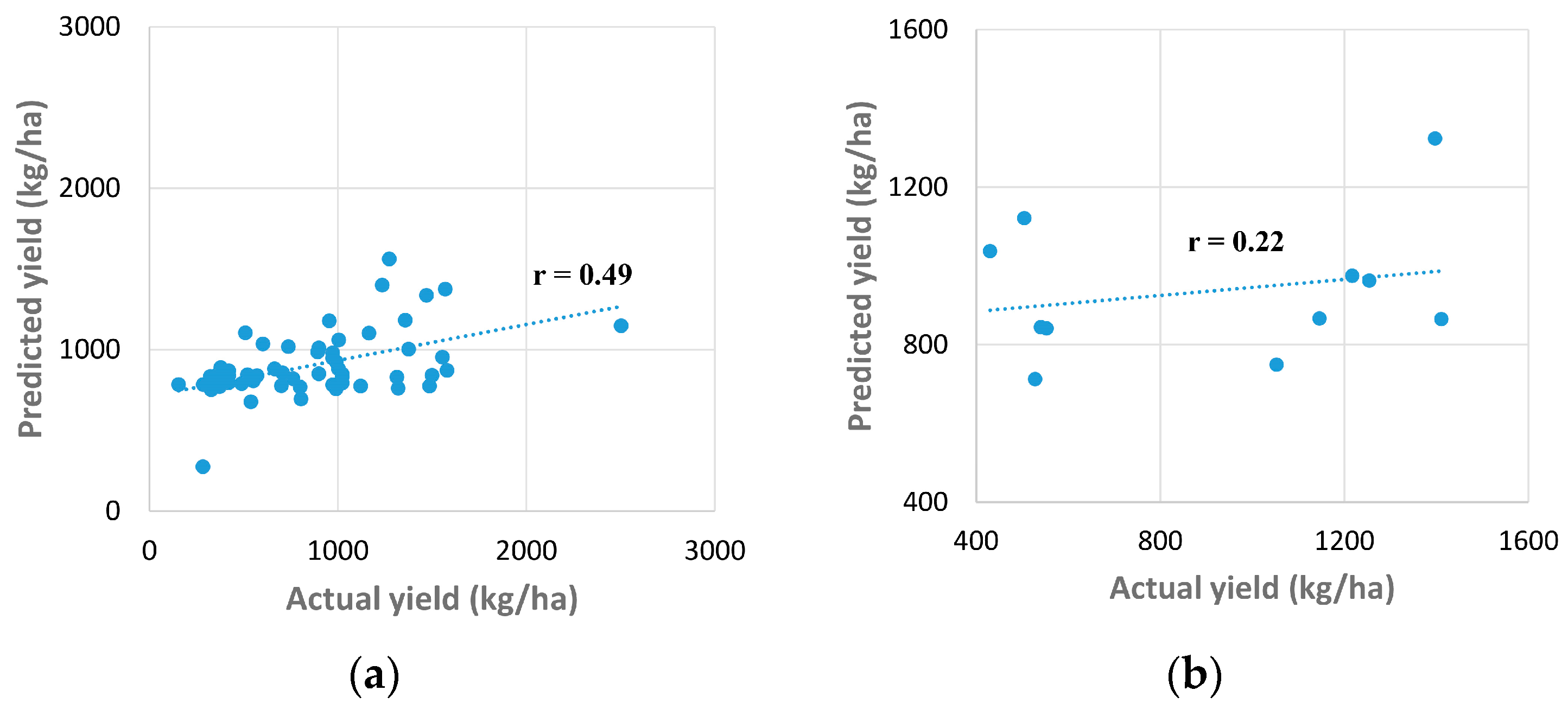
| LM | 0.49 | 0.22 | 0.32 | 0.44 | 153,036.5 | 144,567.3 | 147,216.6 |
| BR | 0.37 | NA | −0.13 | 0.32 | 170,728.1 | NA | 148,876.6 |
| SCG | 0.18 | −0.51 | −0.10 | 0.05 | 203,124.2 | 281,224.0 | 311,886.6 |
| District | Season | Training Algorithm | r | MSE | Num of Epochs | |||
|---|---|---|---|---|---|---|---|---|
| Training | Validation | Test | All Data Points | |||||
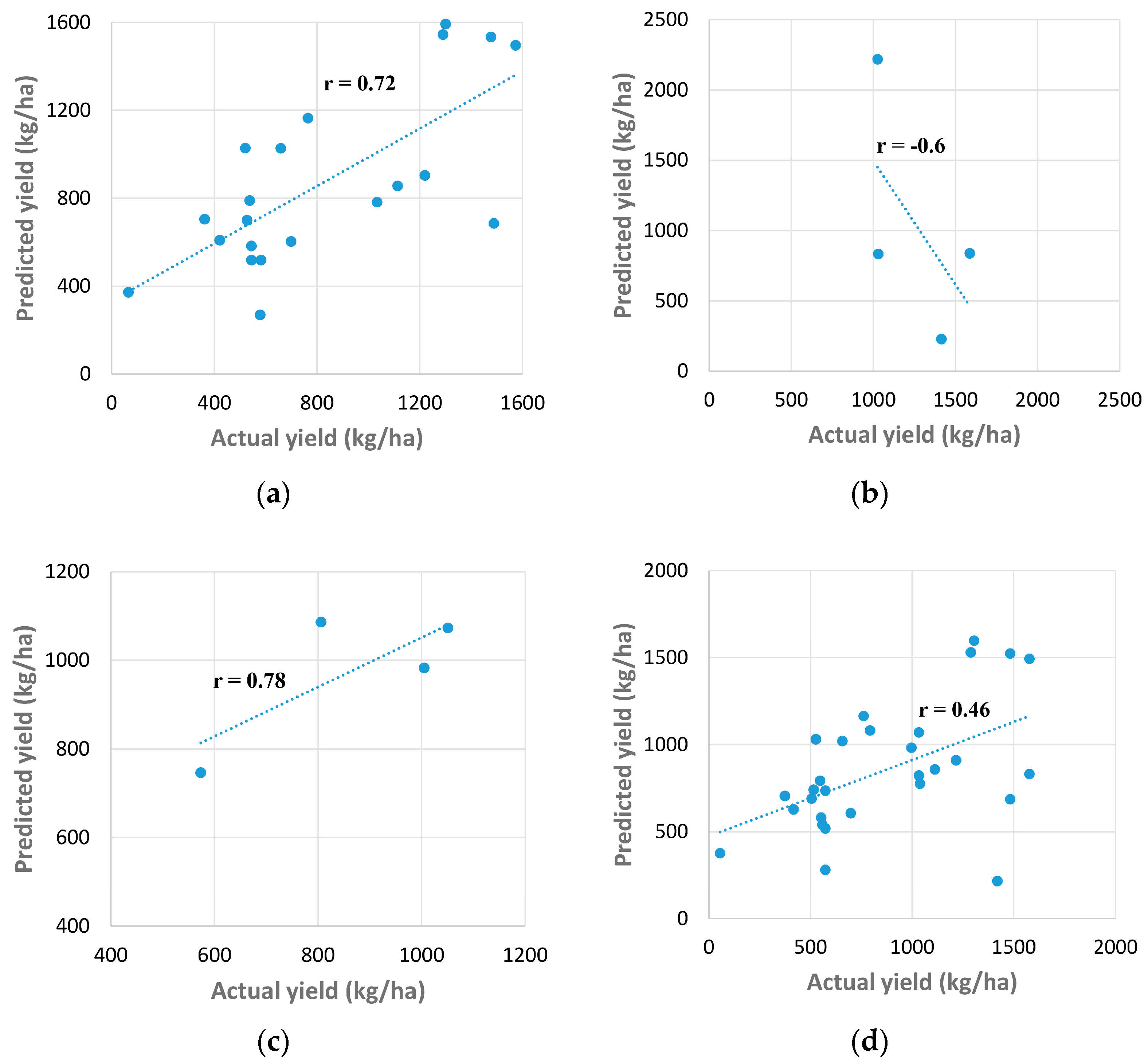
| Anuradhapura | Maha | LM | 0.95 | 0.98 | 0.93 | 0.86 | 0.4993 | 2 |
| BR | 0.99 | NA | 0.1 | 0.89 | 0.0081 | 769 | ||
| SCG | 0.87 | 0.96 | 0.75 | 0.63 | 0.0542 | 12 | ||
| Yala | LM | 1.0 | 0.94 | 0.77 | 0.89 | 0.1902 | 4 | |
| BR | 0.74 | NA | 0.91 | 0.65 | 0.0862 | 87 | ||
| SCG | 0.81 | 0.87 | 0.68 | 0.74 | 0.1721 | 7 | ||
| Badulla | Maha | LM | 0.84 | 0.98 | 0.91 | 0.83 | 0.1113 | 1 |
| BR | 0.82 | NA | 0.95 | 0.8 | 0.2565 | 36 | ||
| SCG | 0.87 | 0.96 | 0.78 | 0.82 | 0.2435 | 06 | ||
| Yala | LM | 0.99 | 0.95 | 0.99 | 0.89 | 0.4007 | 4 | |
| BR | 0.87 | NA | 0.87 | 0.81 | 0.1966 | 1000 | ||
| SCG | 0.84 | 0.88 | 0.93 | 0.84 | 0.2855 | 6 | ||
| Hambantota | Maha | LM | 0.98 | 0.96 | 0.97 | 0.84 | 0.7888 | 02 |
| BR | 0.89 | NA | 0.93 | 0.9 | 0.0804 | 133 | ||
| SCG | 0.98 | 0.93 | 0.99 | 0.94 | 0.1332 | 7 | ||
| Yala | LM | 0.94 | 0.84 | 0.9 | 0.89 | 0.2097 | 2 | |
| BR | 0.87 | NA | 0.76 | 0.84 | 0.1406 | 1000 | ||
| SCG | 0.88 | 0.84 | 0.99 | 0.87 | 0.1397 | 13 | ||
| Kurunegala | Maha | LM | 0.99 | 0.83 | 0.81 | 0.94 | 0.0292 | 3 |
| BR | 0.96 | NA | 0.03 | 0.82 | 0.0247 | 731 | ||
| SCG | 0.94 | 0.82 | 0.55 | 0.76 | 0.0707 | 9 | ||
| Yala | LM | 0.97 | 0.89 | 0.86 | 0.84 | 0.2542 | 1 | |
| BR | 0.84 | NA | 0.87 | 0.81 | 0.2492 | 180 | ||
| SCG | 0.85 | 0.98 | 0.70 | 0.77 | 0.9202 | 06 | ||
| Puttalam | Maha | LM | 0.99 | 0.86 | 0.98 | 0.92 | 0.3919 | 2 |
| BR | 0.54 | NA | 0.55 | 0.57 | 0.6876 | 2 | ||
| SCG | 0.65 | 0.63 | 0.53 | 0.58 | 0.9212 | 4 | ||
| Yala | LM | 0.99 | 0.96 | 0.88 | 0.76 | 0.9067 | 3 | |
| BR | 0.47 | NA | 0.8 | 0.48 | 0.4712 | 2 | ||
| SCG | 0.82 | 0.61 | 0.72 | 0.6 | 0.2909 | 10 | ||
| Algorithms | r | MSE (kg/ha) | |||
|---|---|---|---|---|---|
| Training | Validation | Testing | All Data Points | Validation | |
| LM | 0.45 | 0.37 | 0.19 | 0.33 | 211,778.0 |
| BR | 0.36 | 0.09 | 0.22 | 0.27 | 383,710.9 |
| SCG | −0.01 | 0.20 | −0.07 | −0.03 | 253,457.4 |
| Algorithms | R | MSE (kg/ha) | ||||
|---|---|---|---|---|---|---|
| Training | Validation | Testing | All Data Points | Validation | ||
| Scenario 2 | 0.10 | 0.77 | 0.99 | 0.30 | 82,393.9 | |
| Scenario 3 | 0.99 | 0.78 | 0.69 | 0.77 | 535,600.9 | |
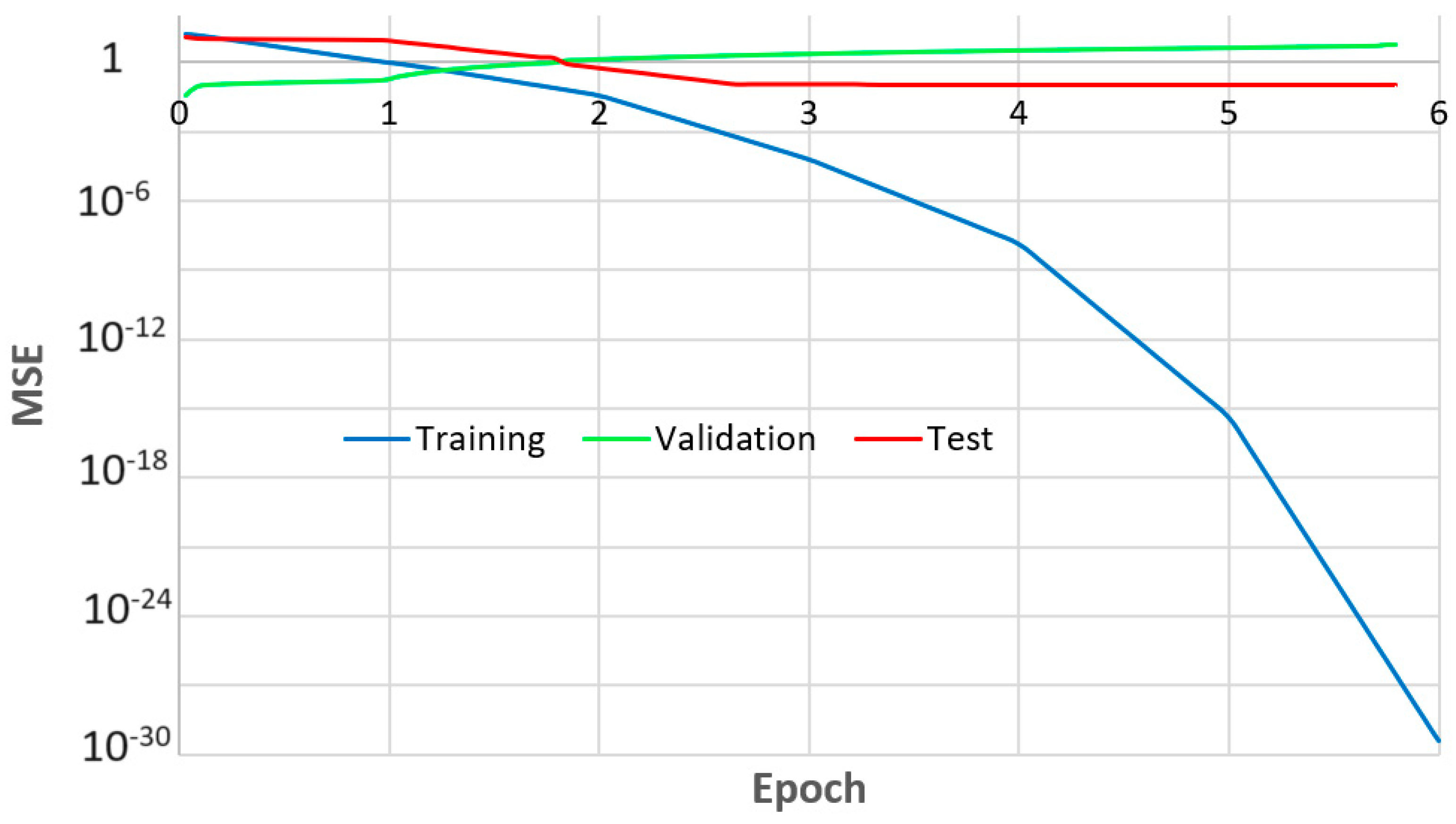
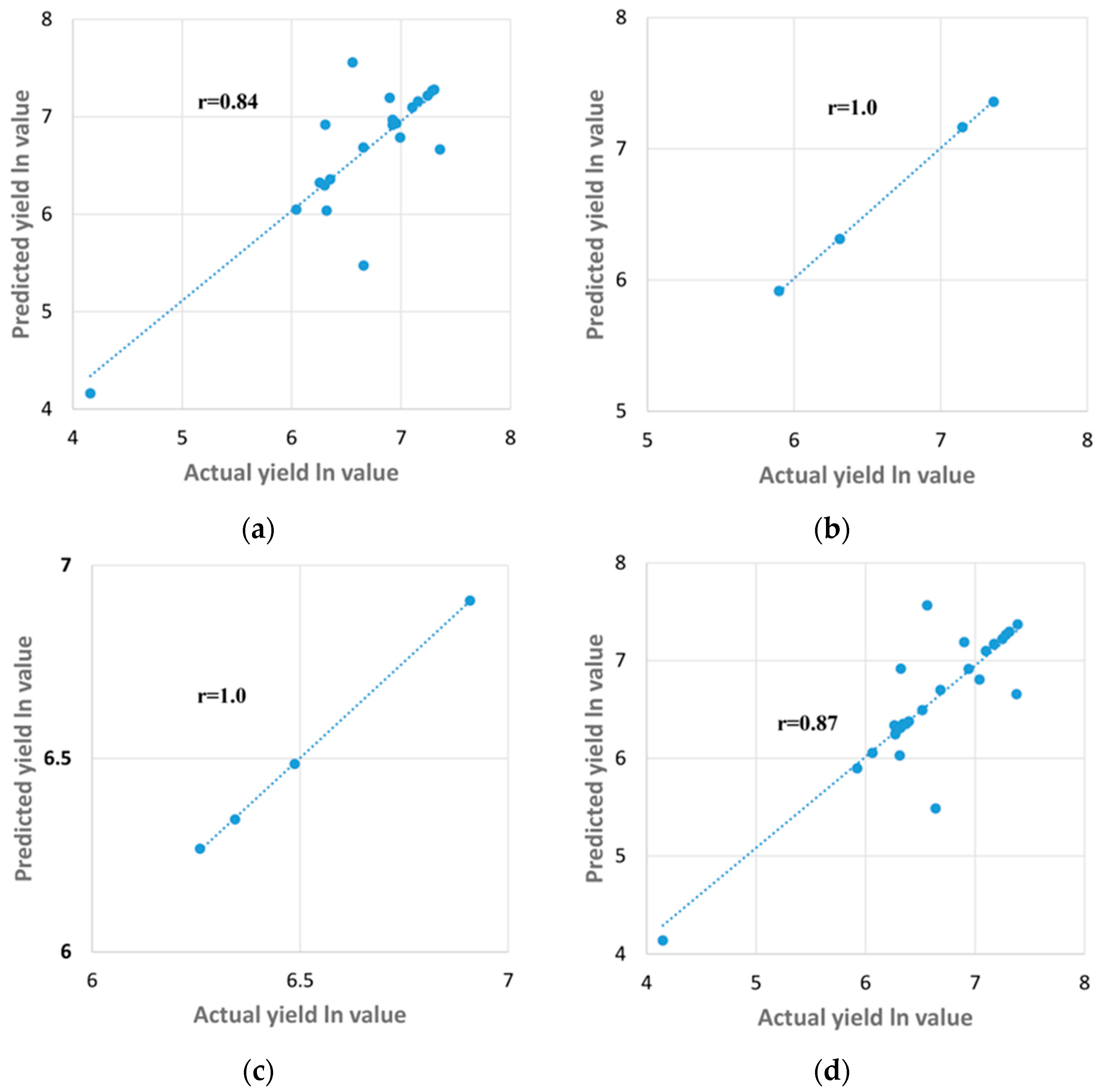
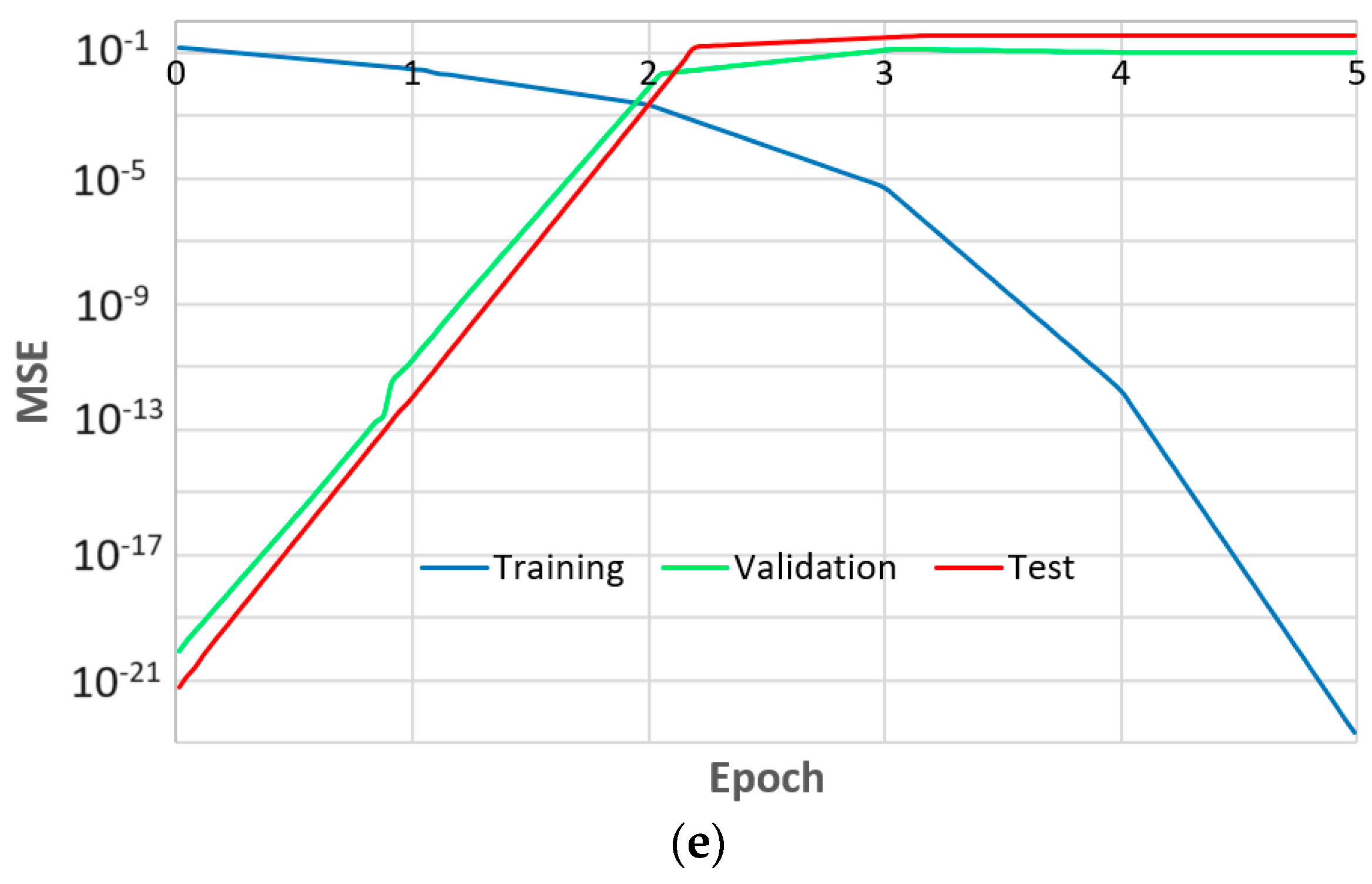
| Scenario 4 | 0.84 | 1.00 | 1.00 | 0.87 | 2.2859 × 10⁻²¹ | |
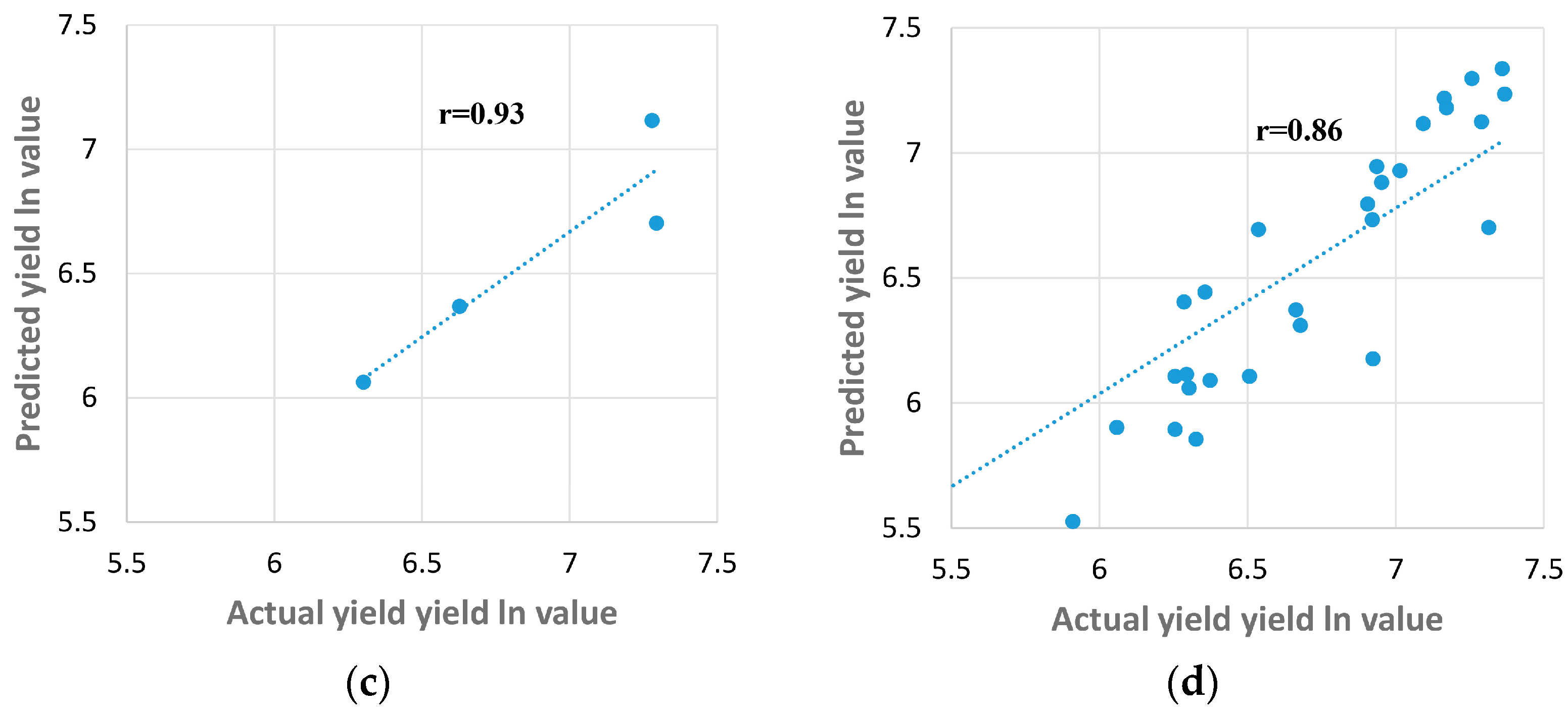
| District | Season | Training Algorithm | r | MSE | Num. of Rpochs | |||
|---|---|---|---|---|---|---|---|---|
| Training | Validation | Test | All Data Points | |||||
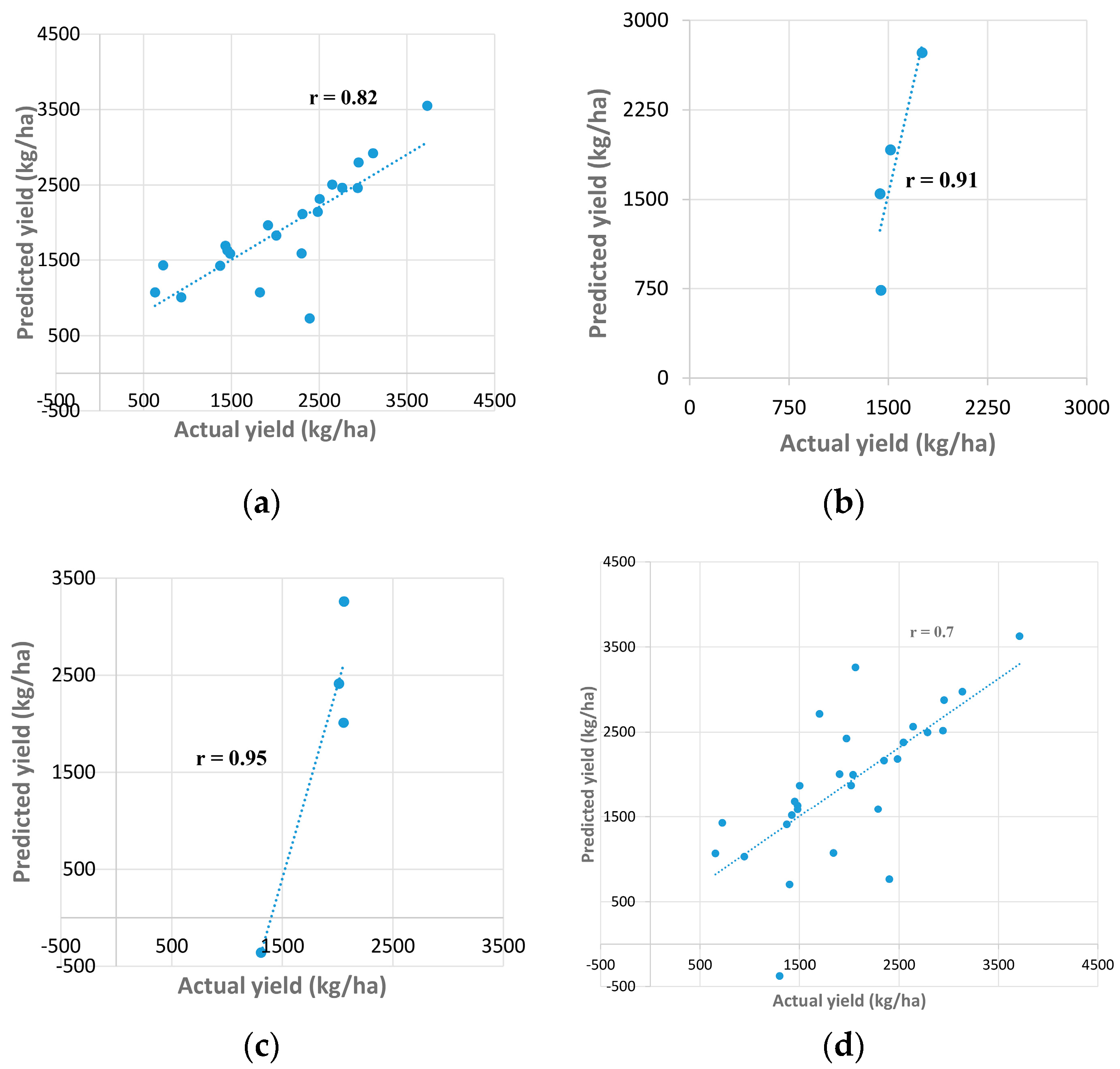
| Anuradhapura | Maha | LM | 0.84 | 1.00 | 1.00 | 0.87 | 2.2859 × 10⁻²¹ | 00 |
| BR | 0.32 | 0.14 | 0.81 | 0.23 | 0.1900 | 01 | ||
| SCG | 0.91 | 0.86 | 0.97 | 0.76 | 0.9616 | 27 | ||
| Yala | LM | 0.99 | 0.94 | 0.98 | 0.95 | 0.0928 | 02 | |
| BR | 0.68 | 0.13 | 0.35 | 0.50 | 0.2489 | 01 | ||
| SCG | 0.24 | 0.96 | 0.53 | 0.42 | 0.0488 | 00 | ||
| Badulla | Maha | LM | 0.94 | 0.92 | 0.63 | 0.89 | 0.2890 | 02 |
| BR | 0.75 | 0.88 | 0.85 | 0.64 | 0.4318 | 02 | ||
| SCG | 0.74 | 0.85 | 0.40 | 0.71 | 0.2618 | 04 | ||
| Yala | LM | 0.76 | 0.87 | 0.86 | 0.77 | 0.2776 | 00 | |
| BR | 0.78 | 0.93 | 0.46 | 0.76 | 0.2831 | 00 | ||
| SCG | 0.70 | 0.53 | 0.66 | 0.68 | 0.7562 | 01 | ||
| Hambantota | Maha | LM | 0.72 | 0.99 | 0.99 | 0.81 | 0.0070 | 00 |
| BR | 0.71 | 0.41 | 0.88 | 0.67 | 0.3920 | 02 | ||
| SCG | 0.99 | 0.99 | 0.41 | 0.93 | 0.0038 | 32 | ||
| Yala | LM | 0.86 | 0.84 | 0.94 | 0.86 | 0.1520 | 0 | |
| BR | 0.68 | 0.93 | 0.54 | 0.60 | 0.5087 | 16 | ||
| SCG | 0.56 | 0.78 | 0.91 | 0.57 | 0.4400 | 01 | ||
| Kurunegala | Maha | LM | 0.90 | 0.99 | 1.00 | 0.94 | 0.0010 | 00 |
| BR | 0.58 | 0.83 | −0.34 | 0.34 | 0.0599 | 20 | ||
| SCG | 0.84 | 0.85 | 0.87 | 0.82 | 0.1204 | 00 | ||
| Yala | LM | 0.99 | 0.85 | 0.78 | 0.92 | 0.5239 | 03 | |
| BR | 0.57 | 0.88 | 0.55 | 0.65 | 1.3866 | 01 | ||
| SCG | 0.66 | 0.94 | 0.10 | 0.67 | 0.2908 | 00 | ||
| Puttalam | Maha | LM | 0.74 | 0.96 | 0.87 | 0.70 | 0.3689 | 01 |
| BR | 0.43 | 0.60 | 0.34 | 0.41 | 0.8918 | 00 | ||
| SCG | 0.75 | 0.99 | 0.53 | 0.70 | 0.1296 | 00 | ||
| Yala | LM | 0.76 | 0.94 | 0.99 | 0.78 | 0.0581 | 00 | |
| BR | 0.27 | −0.13 | 0.93 | 0.34 | 0.2900 | 00 | ||
| SCG | 0.92 | 0.99 | −0.50 | 0.57 | 0.0504 | 20 | ||
| Scenario | K Value | Best Model | MSE |
|---|---|---|---|
| Scenario 1 | 5 | Robust Linear | 1.8071 × 10⁵ |
| Scenario 2 | Linear SVM | 1.3371 × 10⁵ | |
| Scenario 3 | Linear SVM | 2.7491 × 10⁵ | |
| Scenario 4 | Medium Gaussian SVM | 0.37245 |
| Districts | Season | K Value | Best Model | MSE |
|---|---|---|---|---|
| Anuradhapura | Maha | 5 | Gaussian SVM | 0.37245 |
| Yala | Bagged Trees | 0.1738 | ||
| Badulla | Maha | 5 | Bagged Trees | 0.46631 |
| Yala | Coarse Gaussian SVM | 0.50422 | ||
| Hambantota | Maha | 5 | Fine Tree | 0.17157 |
| Yala | Linear SVM | 0.46875 | ||
| Kurunegala | Maha | 5 | Coarse Tree | 0.26792 |
| Yala | Bagged Trees | 0.73634 | ||
| Puttalam | Maha | 5 | Gaussian SVM | 0.45825 |
| Yala | Coarse Tree | 0.45147 |
| References | Description | Employed Methodology | Remarks (Comparison with the Study) |
|---|---|---|---|
| [12] | Using climatic factors, paddy yield was predicted and evaluated using training models to train ANNs for 8 districts in Sri Lanka. | ANN model trained using LM, BR and SCG training algorithms | This research was conducted using one method. However, in our study, we expanded the scope by applying two distinct methods and subsequently validated their outcomes through K-Fold cross-validation. |
| [58] | In this study, artificial intelligence technology was employed for forecasting in dynamic climatic scenarios, incorporating historical arboreal data and insights from an ecological process-oriented model. | Growth and yield models and JABOWA-3 | Our study utilized only actual climatic data from previous years to train an ANN model. Furthermore, our investigation encompassed the application of two distinct analytical methods. In addition to this, the K-Fold cross-validation technique was employed to validate both methods. |
| [59] | The aim of this study was to assess how climate change affects the grain yield of rainfed wheat in the Kashafrood basin located in northeastern Iran. | Hadley Centre Coupled Model, version 3 (HadCM3) And Canadian Climate Centre for Modelling and Analysis, version 2 (CGCM2) | We used actual climatic data from previous years and the main goal was to understand the connection between climatic factors and groundnut yield. Given the inherent attributes of ANNs, such as their flexibility, adaptability, data-driven analytical capabilities, enhanced predictive accuracy, and the ability to calibrate and correct biases in models, we concluded that the ANN model was the most suitable approach for our research compared to HadCM3 and CGCM2. |
| [60] | This study, conducted over a 20-year period from 1993 to 2013, assessed the impact of climatic factors, such as monthly rainfall and temperature, on sugarcane productivity in Maharashtra, revealing a non-linear relationship that varies seasonally. | Multiple Regression Model | In our study, we utilized the ANN model, known for its suitability in identifying non-linear relationship patterns. Furthermore, we extended the inclusion of climatic factors across Scenarios 1–4 as input variables and employed two distinct methods. |
Disclaimer/Publisher’s Note: The statements, opinions and data contained in all publications are solely those of the individual author(s) and contributor(s) and not of MDPI and/or the editor(s). MDPI and/or the editor(s) disclaim responsibility for any injury to people or property resulting from any ideas, methods, instructions or products referred to in the content. |
© 2023 by the authors. Licensee MDPI, Basel, Switzerland. This article is an open access article distributed under the terms and conditions of the Creative Commons Attribution (CC BY) license (https://creativecommons.org/licenses/by/4.0/).
Share and Cite
Sajindra, H.; Abekoon, T.; Wimalasiri, E.M.; Mehta, D.; Rathnayake, U. An Artificial Neural Network for Predicting Groundnut Yield Using Climatic Data. AgriEngineering 2023, 5, 1713-1736. https://doi.org/10.3390/agriengineering5040106
Sajindra H, Abekoon T, Wimalasiri EM, Mehta D, Rathnayake U. An Artificial Neural Network for Predicting Groundnut Yield Using Climatic Data. AgriEngineering. 2023; 5(4):1713-1736. https://doi.org/10.3390/agriengineering5040106
Chicago/Turabian StyleSajindra, Hirushan, Thilina Abekoon, Eranga M. Wimalasiri, Darshan Mehta, and Upaka Rathnayake. 2023. "An Artificial Neural Network for Predicting Groundnut Yield Using Climatic Data" AgriEngineering 5, no. 4: 1713-1736. https://doi.org/10.3390/agriengineering5040106