Modelling the Temperature Inside a Greenhouse Tunnel

Abstract

Climate-change-induced unpredictable weather patterns are adversely affecting global agricultural productivity, posing a significant threat to sustainability and food security, particularly in developing regions. Wealthier nations can invest substantially in measures to mitigate climate change’s impact on food production, but economically disadvantaged countries face challenges due to limited resources and heightened susceptibility to climate change. To enhance climate resilience in agriculture, technological solutions such as the Internet of Things (IoT) are being explored. This paper introduces a digital twin as a technological solution for monitoring and controlling temperatures in a greenhouse tunnel situated in Stellenbosch, South Africa. The study incorporates an aeroponics trial within the tunnel, analysing temperature variations caused by the fan and wet wall temperature regulatory systems. The research develops an analytical model and employs a support vector regression algorithm as an empirical model, successfully achieving accurate predictions. The analytical model demonstrated a root mean square error (RMSE) of 2.93 °C and an $R^2$ value of 0.8, while the empirical model outperformed it with an RMSE of 1.76 °C and an $R^2$ value of 0.9 for a one-hour-ahead simulation. Potential applications and future work using these modelling techniques are then discussed.

1. Introduction

Thermal modelling in greenhouse tunnels is paramount for optimising agricultural productivity. These models—the focus of this paper—simulate temperature variations, helping farmers make informed decisions about ventilation, heating, and crop management. By accurately predicting temperature fluctuations, growers can mitigate risks associated with extreme weather, ensuring optimal conditions for plant growth.

Climate change significantly hampers global agricultural productivity, characterised by erratic rainfall patterns, extreme temperatures, and prolonged droughts, posing a substantial risk to global food security [1,2,3,4,5,6]. This challenge is particularly pronounced in under-resourced countries where governments and private agencies face increasing difficulties coping with climate-induced food insecurity. Africa, heavily reliant on rainfall for irrigation, is projected to be the most adversely affected continent [7,8,9,10]. Farmers often depend on short-term weather patterns and forecasts, exacerbating the vulnerability of the agricultural sector to the impacts of climate change [11,12].

Recognising the imperative for transformative measures, the agricultural sector must shift from conventional practices to technology-based solutions to meet the growing global population’s food demand [13]. The adoption of innovative technologies can enhance food production sustainably, addressing challenges such as hunger and malnutrition [14,15]. Countries like Japan and Abu Dhabi have successfully implemented climate-smart farming practices, with Abu Dhabi’s agricultural sector contributing significantly to the country’s GDP [16,17].

Despite the potential benefits, the adoption of climate-smart farming practices in African countries lags behind the severity of climate change impacts. The incorporation of these technologies could not only mitigate the adverse effects on agriculture but also uplift the socioeconomic status of those dependent on farming for survival. Given the agricultural sector’s prominent role in African countries’ GDP, embracing climate-smart technologies becomes crucial for fostering resilience and sustainable growth.

This paper emphasises the urgency of adopting climate-smart farming practices, drawing attention to successful implementations in other regions. It highlights the economic benefits witnessed in Abu Dhabi, showcasing the potential positive impact on GDP. The slow adoption in African countries is underscored, urging expedited integration to effectively address the challenges posed by climate change on agricultural systems and the broader economy.

One such climate-smart farming method is precision agriculture (PA). It introduces a dynamic relationship between sensor data and agriculture. Through feedback control systems, data can aid the growing of certain crops under specific conditions. These conditions can be controlled by researchers through the use of actuators and different types of sensors. The Internet of Things (IoT) has revolutionised precision agriculture by connecting sensors to the internet for remote access and dataset creation [18].

This paper presents a piece in the PA puzzle—an empirical (data-based) and analytical (physics-based) thermal model is presented that accurately models the ambient temperature inside a greenhouse tunnel.

2. Related Works

2.1. Precision Agriculture Adoption

PA systems vary based on their application and the desired growing conditions. Therefore, applications are diverse and can encompass multiple different technologies. Eloquently described by Lowenberg-DeBoer and Erickson [19], PA is more of a toolkit that farmers can use for their specific needs. According to Montzka et al. [20], standard agricultural practices in the agricultural sector are responsible for 13.5% of greenhouse gas (GHG) emissions in the world. Worryingly, two-thirds of all methane production occurs from agriculture and the burning of fossil fuels. Through the use of fertiliser that is rich in nitrous oxide, agriculture also contributes to large quantities of NO₂ waste in the environment due to losses when not all of the fertiliser is used. Montzka et al. [20] further suggest that these large losses can be reduced by reducing the amount of fertiliser used. However, as discussed by Balafoutis et al. [21], research shows that the use of PA systems can mitigate the effects of climate change through the control of GHG emissions. PA systems can positively contribute mainly through the management of nutrient application (such as $N{O}_2$ waste reduction) in agriculture and through direct control of resources in crop production. Mabitsela et al. [22] used an aeroponics system in Stellenbosch, South Africa, to prove that the use of aeroponics in an African context can yield better results compared to traditional growing methods and provide sustainable growing methods. The use of soilless cultivation proved successful in terms of improved yield, and also in terms of energy and water conservation. Furthermore, the use of temperature sensors in the study by Mabitsela et al. [22] created a climate-smart environment for the experiment to have optimum growing conditions. Further, climate-smart agriculture (CSA) is explored in Mizik et al. [23] with an emphasis on how small-scale farmers can adopt CSA practices. They identify that CSA technological solutions should be developed on a case-by-case basis due to the differing environments and necessities of the farm. CSA adoption not only relates to technological use but also smart farming choices like crop rotations. In Doyle et al. [24], a CSA aquaponics system is developed to simultaneously grow fish and vegetables in East Africa. Although their system is not technologically advanced, as a simple water circulation system is used, there is potential for technological integration using the IoT for prediction and control of the amount of water used in the system.

Despite the potential benefits of IoT adoption in agriculture, Sub-Saharan Africa lags behind developed countries in embracing this technology [25]. Recognising the economic potential, particularly in rural areas heavily dependent on agriculture, the integration of IoT technology is crucial. An example highlighted by Nigussie et al. [26] involves a farm in northern South Africa, where an irrigation solution was proposed to solve the use of excessive water. A digital twin was developed using sensor data to optimise irrigation, reducing resource consumption without adversely impacting on crop yield. This not only leads to immediate economic gains but also ensures long-term sustainability in on-farm practices, demonstrating the transformative potential of IoT technologies in agriculture. In China, Zhang et al. [27] explored the optimization problem of improved agricultural output while minimizing energy consumption. They argue for the development of an agriculture energy internet (AEI). This involves using agricultural and renewable energy models to develop digital twins for the aforementioned optimization problem. By utilizing multiple different types of sensors for both agricultural and energy attributes such as temperature and power consumption, the trade-offs of improved agricultural production and increased energy consumption can be explored. Although this study does not focus on the electrical energy aspect, it contributes to the development of similar digital twin solutions for yield optimization in agriculture. An example of this comes from Fu et al. Fu and Zhou [28] accomplished the above problem by combining electrical energy models and the modelling of agricultural systems in a single model.

A study by Jans-Singh et al. [29] compared the performance of the static seasonal autoregressive moving average model (SARIMA) and the dynamic linear model (DLM), using sensor data captured by a digital twin. The SARIMA model, trained solely on temperature data, outperformed the DLM in the morning forecast, while the DLM excelled when LED lights were activated in the afternoon.

Similarly, Patil et al. [30] explored the autoregression model (AR), neural network autoregressive model (NNARX), and autoregressive moving average model (ARMAX) for predicting internal greenhouse temperature. The NNARX model, incorporating non-linear parameters, outperformed other linear models.

In Morocco, Allouhi et al. [31] developed regression models for netted greenhouses, comparing Gaussian predictive (GP) models with support vector regression (SVR) in linear and quadratic forms. While the GP model achieved high accuracy, the quadratic SVR and linear SVR also performed acceptably. Notably, models assuming non-linearity or, specifically, modelling produced the most accurate results across these studies.

In summary, the application of digital twins in agriculture involves sophisticated modelling techniques, with studies showcasing the superiority of non-linear algorithms in accurately predicting variables like temperature, essential for precision farming.

2.2. Analytical Models

Thermal modelling of greenhouse tunnels involves a number of non-linearities due to a number of factors, including: ambient air temperature outside of the tunnel, solar radiation, wind speed, orientation, size, and especially whether or not the sides of a tunnel are open or closed. Because of these non-linearities, even the physical characteristics (shape, size, orientation) of the tunnel affect the internal temperatures. In [32], the authors used Computational Fluid Dynamics (CFD) software to model a greenhouse based on its shape (chapel or dome-shaped) and compared the effects of solar radiation and wind on the internal temperatures. They concluded that the dome-shaped tunnel was more aerodynamic, causing less drag during high-speed winds, and a lower difference between the outside and inside temperatures.

Similarly, Mobtaker et al. [33] used multiple different orientations and shapes of greenhouses to determine optimal conditions for energy saving in a greenhouse. Unlike Nauta et al. [34], they investigated the effect that variables inside of a greenhouse have on one another. Using radiation networks, they [33] describe the effects that the greenhouse cover, soil, and a brick wall they placed on the north wall of the greenhouse have on each other. They determined that, in fact, the solar radiation incident on the top soil and front face of the brick wall causes the largest rise in internal temperatures. In terms of the error between their modelled values and the measured values, their model for the inside air had an $R^2$ value of $0.9$ and an RMSE (in °C) of 2.82 °C. Despite the importance of understanding the impact of the geometry and orientation of the greenhouse, it is also important to place emphasis on the effect that solar radiation has on the interior temperatures. Understanding the effect of outside temperatures on inside temperatures allows for better decision making for farmers and researchers, rather than the effect of soil or outside walls.

In Tadj et al. [35], a study conducted in 2006, the authors explored the use of CFD to analyse the dynamics of heating pipes in a greenhouse tunnel. Their CFD model was presented as a 3D model. The authors argue the use of these models in this context, as the placement of these heating pipes in greenhouse tunnels had not been explored prior to their research. The results show that the experiment proved a previous assumption in greenhouse tunnels that temperature distributions in tunnels are largely due to air flow patterns within the tunnel. This is important to note as the greenhouse tunnel used in our study uses an industrial fan and wet wall to control air flow in the tunnel and to produce a cooling effect in the tunnel. The authors used an experimental site in Greece, which has a Mediterranean climate like the Western Cape in South Africa. Therefore, their study is representative of what to expect regarding the temperature dynamics of the greenhouse tunnel being used in this paper.

Nauta et al. [34] explored the thermal modelling of an open-sided greenhouse tunnel in Guelph, Canada. They argue that CFD models are able to predict only one operational condition in a greenhouse tunnel, while being computationally intensive and are particularly difficult to compute without initial conditions. Their solution was to create a one-dimensional lumped-capacitance model that separates the tunnel into multiple layers with different heat transfer equations for each layer. Their aim was to predict the air and soil temperature within the tunnel using this physics-based model. Their results show an RMSE for the soil temperature to be 4.28 °C and 4.25 °C for air temperature. Although these results were captured in Canada, a much colder region than South Africa, the results show that using a lumped-capacitance model can accurately predict the internal conditions of a tunnel even with a minor error. Although the present study mainly explores data-driven modelling, the results will be able to justify the means of physics-based prediction models in a hotter climate, and will be a good comparison against the data-driven model.

Comparatively, a computationally aided CFD model using “Ansys” was demonstrated in Tong et al. [36]. In China, greenhouses that use solar radiation for internal heating are named solar greenhouses and are a focus in research due to the need for large-scale food production throughout the year. The authors argue that previous research (before 2009) used numerical modelling and a lumped-capacitance model to model internal temperatures. However, they argue that the accuracies of these models decline as the temperature variations in these greenhouses are dynamic in space and time. The authors used extensive heat transfer equations to numerically model the interior temperatures of this greenhouse. They developed two models: one for during the day and one for during the night. A total of 52 temperature sensors were placed in the greenhouse at different depths in the soil and at various heights within the tunnel. In conjunction with a pyranometer measuring the solar radiation, both climatic conditions were sampled every second, and after 600 s, the average was calculated. Their final results showed a highly accurate analytical model with a difference of 1.0 °C for the nighttime model, and a 1.5 °C difference for the daytime model. Noteworthy findings included the temperature of the soil and plastic film of the greenhouse being higher than that of the ambient air inside the greenhouse throughout the day, showing that more energy is stored in these layers of the tunnel rather than the air. It is clear that this model is highly complex and requires numerous considerations to produce a highly accurate model. In total, 20 different equations with multiple boundary conditions were used in the CFD modelling software to produce the model. Although accuracy is important for these models, it is noteworthy how relatively less equipment is used in lumped-capacitance models, such as in Nauta et al. [34], to produce errors of about 4.25 °C.

In Tacarindua et al. [37], the authors used different temperature gradients varying from 1 to 3 °C above ambient temperature to monitor the growth of soybeans and reported 30% yield losses at temperatures above 3 °C. Therefore, predicting these temperatures, even through lumped-capacitance modelling, can still result in improvements in yield. In the South African context, where these models are lacking, any increase in yield would be economically and productively beneficial.

2.3. Empirical Data-Driven Models

Digital twins play a crucial role in agriculture, encompassing data collection from sensors, control of actuators, and modelling. The latter, modelling, could be vital for predicting outcomes, and can be analytical (based on physics and heat transfer equations) or empirical (utilising datasets in machine learning algorithms). Linear regression models, known for their simplicity and accuracy, assume a linear relationship between the input and output variables, which could be risky when the physical (physics) relationship is not known. To address this, algorithms like Generalised Regression Neural Networks, capable of modelling non-linearities, have been developed.

Finally, we developed a neural network model for a separate study using the data in this study, which is detailed in Jogunola et al. [38]. A Convolutional Neural Network (CNN), Long Short-Term Memory (LSTM), and a hybrid of CNN and Bidirectional LSTM (BLSTM) were developed to predict temperatures within the greenhouse. The results showed an average mean squared error of 0.025 °C for all of the models.

2.4. Performance Metrics

In both analytical and empirical modelling in the literature, common performance metrics are used to compare the accuracy and predictive ability of the proposed models. These metrics include root mean square error (RMSE), $R^2$, mean absolute error (MAE), and mean bias error (MBE).

2.4.1. RMSE

RMSE is the average error between the predicted and actual value in a model. This is represented by the formula:

$$RMSE=\sqrt{\frac{1}{n}\sum _{i=1}^n{(y_i-{\widehat{y}}_i)}^2}$$

(1)

where n is the number of predictions or available measured values, $y_i$ is the actual measured value, and ${\widehat{y}}_i$ is the predicted or regressed value.

2.4.2. $R^2$

Commonly known as the coefficient of determination, this metric is a good measure of how well the model fits the data. Its formula is:

$$R^2=1-\frac{RSS}{TSS}$$

(2)

where $RSS$ represents the residual sum of squares, or the sum of the error or bias term in a regression model, and $TSS$ represents the total sum of squares of the error between $y_i$ and ${\widehat{y}}_i$ as shown in Equation (1).

2.4.3. MAE

Similarly to RMSE, MAE is a measure of the difference between the measured and the predicted. The main difference is that this metric is not square rooted and the absolute error is summed and averaged from the number of observations.

$$MAE=\frac{1}{n}\sum _{i=1}^n|y_i-{\widehat{y}}_i|$$

(3)

2.4.4. MBE

MBE represents the bias of the predicted values, as in whether a predicted value is underpredicted or overpredicted represented by a negative or positive MBE, respectively.

$$MBE=\frac{1}{n}\sum _{i=1}^n(y_i-{\widehat{y}}_i)$$

(4)

3. Thermal Model Development

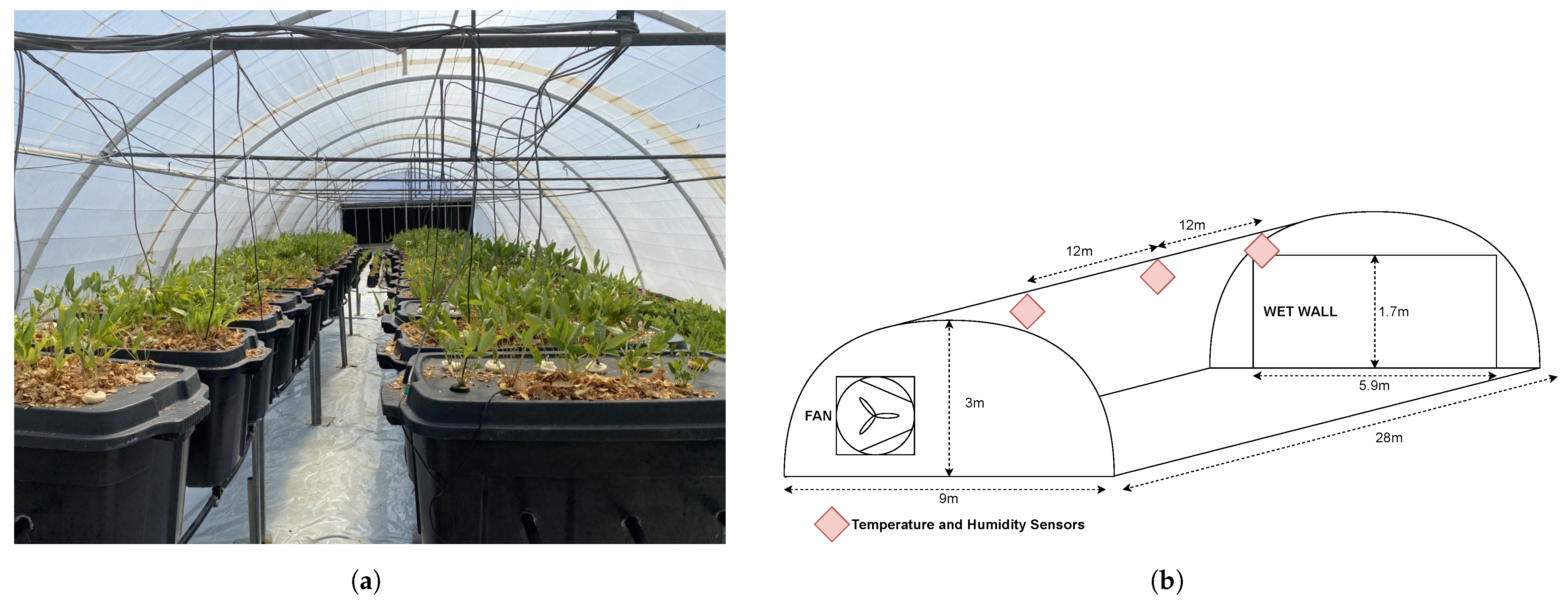
3.1. Tunnel Parameters and Data Acquisition

This study was situated in a closed tunnel at the Welgevallen Experimental Farm, part of Stellenbosch University in South Africa. Data were collected from 18 November to 30 December 2022, spanning a period of 42 days. The tunnel has a dome-shaped structure with dimensions of 28 m in length, 9 m in width, and 3 m in height. Three sensors were strategically placed at twelve-meter intervals, starting from the tunnel entrance and extending to the wet wall. The extraction fan makes up one-third of the wall space adjacent to the tunnel entrance. Figure 1a,b depict the tunnel during an experimental trial and illustrate its layout, respectively.

The tunnel layout, as depicted in Figure 1b, consists of a fan facing east and a wet wall facing west. The fan side of the tunnel, therefore, receives the majority of the sunlight in the morning and afternoon, while the wet wall side receives its sunlight mainly in the afternoon. The aeroponics system is on the fan side of the tunnel closest to the front temperature and humidity sensor as seen in Figure 1b. The ground is covered in a PVC covering to prevent water drainage affecting the trestle tables on which the aeroponics system stands. The setup is tailored to collect data from sensors in three segments of the 28 m tunnel (Figure 1a). Temperature and humidity were measured with DHT22 sensors. They have a temperature range of $-40$ to 80 °C and humidity range of 0 to 100%, and accuracies of ±0.5 °C for temperature and 5% for humidity. We used a Raspberry Pi Model 3B to aggregate sensor data, provide internet connectivity, save a local CSV file on the device, interface with the actuator control mechanisms, and support potential expansions.

Each sensor recorded humidity and temperature readings every minute for a five-minute duration. Thereafter, averages were calculated and stored in the local CSV file. In addition to temperature and humidity data, the timestamps and a binary value (0 or 1) were stored, indicating whether the fan and wet wall were active. At the end of each day, the CSV file was uploaded to the cloud for off-site access.

The temperature in the tunnel was regulated by concurrent control of the extraction fan and wet wall. The middle sensor (Figure 1b), which is approximately 12 m from the fan and 16 m from the wet wall, was used to affect the control. To reduce the potential for spurious readings resulting in erroneous control, the controlling temperature sensor was read 10 times per min, and the median value used to control the fan and wet wall. We empirically determined a hysteresis band for temperature control: below 22 °C, the climate control turned off, and above 30 °C, it turned on. A Solid State Relay (SSR) was used to control the fan and wet wall pump through contactors connected to these actuators. We only used the middle sensor’s temperature readings to develop the analytical and empirical model studied in this paper. Although this reduces the spatial resolution of the data by focusing on a single area of the tunnel, we identified in preliminary results that the biasing from the sides of the tunnel, the fan, and the wet wall produced skewed results. These models therefore focus on giving agricultural researchers and farmers the ability to characterise their greenhouse tunnel in a general sense as to aid decision making as to which crops can and cannot be grown.

3.2. Analytical Thermal Model Development

A physics-based, analytical model is developed with the aim of predicting the internal temperature in the greenhouse tunnel. Kittas et al. [40,41] developed heat transfer equations for evaporative cooling systems similar to that of the greenhouse tunnel studied in this paper. Evaporative cooling is caused by water flowing over cooling pads of a certain material; thereafter, an extraction fan pulls water vapour from these pads into the greenhouse, which causes evaporation, leaving cooler temperatures throughout the tunnel. Kittas et al. [40,41] argue that the internal temperature is affected mainly by six factors: the heat loss coefficient of the tunnel cover, shading inside the tunnel, ventilation rate, water evaporation from the wet wall, plant transpiration, and soil evaporation. However, the last factor is largely neglected in this model. Instead of a time-based model, they developed a model that is dependent on the airflow path in the tunnel, which is longitudinally from the wet wall. The data captured in this present study form a time series, meaning this model can then determine the temperature in the current instant without temporal dependencies assuming a steady state is reached. Furthermore, the data are recorded in five-minute intervals, leading to a reasonable assumption that sudden changes in temperature would reach a steady state in that time interval. Using time series data in this way has the added benefit of using forecasted data (namely for solar radiation and ambient temperature) to describe the internal temperatures of the tunnel. The heat balance equation from Kittas et al. [40,41] is stated as:

$$V\rho C_{p}d{T}_{in}=[\tau (1-\alpha )R_g-\beta e_{s,in}]dx-K_{c}P[T_{in}\left(x\right)-T_o]dx$$

(5)

Equation (5) is corrected for the erroneous exclusion of $\rho$, the air density ($\frac{\mathrm{kg}}{{\mathrm{m}}^3}$), which is written as a subscript of the variable V, the ventilation rate ($\frac{{\mathrm{m}}^3}{\mathrm{s}}$), in Kittas et al. [41]. A list of variables, their units, and their assumed values are described in

Table 1. List of all variables and constants used in the development of the analytical thermal model.

Name	Represents	Constant?	Value	Units
$T_{in}\left(x\right)$	Current temperature at position x from the wet wall	N	*	°C
$T_o$	Outside temperature	N	*	°C
$T_{o,w}$	Wet bulb temperature	N	*	°C
$\alpha$	Plant transpiration rate	Y	0.8	Dimensionless
$\tau$	Transmissivity of the greenhouse cover	Y	0.35	Dimensionless
$R_g$	Solar radiation outside the tunnel	N	*	W/m2
L	Greenhouse width	Y	9	m
P	Roof perimeter	Y	28.2	m
V	Ventilation rate	Y	2	m3/s
$C_p$	Specific heat capacity of air	Y	1005	$\frac{\mathrm{J}}{{\mathrm{kg}}^{\circ }\mathrm{C}}$
$\rho$	Air density	Y	1.14	$\frac{\mathrm{kg}}{{\mathrm{m}}^3}$
$K_c$	Heat loss coefficient of greenhouse cover	Y	3	W/m2 °C
$\eta$	Cooling efficiency	Y	0.3	Dimensionless

* Time-variant variables.

.

Through numerous simplifications and assumptions, including the assumption that solar radiation has the largest effect on the internal temperature as compared to the evapotranspiration process in the plants and soil, the final model equation becomes:

$$T_{in}\left(x\right)=T_o+[-\eta (T_o-T_{o,w})-A1]e^{(-A2x)}+A1$$

(6)

where:

$$A1=\frac{\left[\tau (1-\alpha )R_g\right]L}{K_{c}P}$$

(7)

and:

$$A2=\frac{K_{c}P}{V\rho C_p}$$

(8)

A1 and A2 were erroneous in Kittas et al. [41] compared to their original derivation in Kittas et al. [40] and were corrected for their mistake in Equations (7) and (8).

In Kittas et al. [40,41], the parameters chosen for their model were optimised to best fit their measured data and their greenhouse. However, their greenhouse had a different orientation and size and could not be used for the parameters in this model. Therefore, the results from the parameter optimisation for the model in this paper were relatively close to those seen in Kittas et al. The transmissivity of the greenhouse cover, $\tau$, was expected to be higher as the greenhouse’s internal temperatures were heavily influenced by solar radiation. A large portion of the solar radiation, however, is potentially absorbed by the greenhouse cover, or is reflected back into the surrounding space. $\alpha$, the plant transpiration coefficient, was much higher than that in [41], which may be due to the black containers in the aeroponics system and various control crops used in the trial inside the tunnel. For V, the ventilation rate, the optimisation found 2 m³/s to be the best choice for the model, which is close to the 2.4 m³ s based on the fan’s advertised ventilation rate [42]. The heat loss coefficient, $K_c$, was 3 W/m²³ °C, whereas the value used in [41] was 4.2 W/m² °C. This is expected as a different covering to that in Kittas et al. was used [41]. Finally, $\eta$, the cooling efficiency of the wet wall, was unexpectedly 0.3 compared to the 0.8 that Kittas et al. used. This inefficiency may be due to the age of the wet wall that led to a lower cooling efficiency.

Due to the model being dependent on the fan state, a simulation was run using the analytical model’s energy balance equation and model parameters to predict the fan state. This is due to the ventilation rate of the tunnel reducing to 0 m³/s when the fan is off, which directly affects the model. The simulation process is as follows:

• Take the current time step’s outside temperature and solar radiation, with the first recorded instance of the fan state to predict the inside temperature.
• Use this prediction with the previous fan state to simulate the fan being on or off.
• Predict the next inside temperature.
• Store the simulated fan state and predicted temperature in an array to be exported at a later stage.

3.3. Empirical Data-Driven Model Development (Support Vector Regression)

A data-driven model was developed using the measured data. The measured data were augmented with irradiation (W/m²) and ambient temperature, both sampled hourly, from MeteoBlue© [43] for the town. To account for the fact that the measured data were in five minute intervals, and those of MeteoBlue© were hourly, the hourly data were linearly interpolated into five minute intervals for better training with the other input features that were also in five minute intervals.

Finally, since the two sensors at the entrance and rear of the tunnel are influenced by their proximity to the fan or the wet wall, the model to predict the ambient temperature inside the tunnel was developed using only the middle sensor. This sensor is also adequate for model development as the majority of the crops are in the area of this sensor.

The regression model served dual purposes: first, it was employed to generate predictions for the next five minutes, and second, the anticipated temperature was used as an input for the model to simulate conditions within the tunnel. An SVR was developed to predict internal temperatures and the fan and wet wall state. The input features for these models were previous inside temperature ($T[n-1]$), previous outside temperature ($T[n-1]$), solar radiation (W/m²), and climate control (fan and wet wall) status (on or off). The dataset used an 80:20 split to train and test the model, with model parameters being optimised using the training set only. The results, as shown in the results section below, are only the test set results of both the analytical and empirical model. We published the data, including the models’ outputs in Hull et al. [44].

Support Vector Regression (SVR) is an efficient choice for regression owing to its swift computation and the assumption that data are non-linear. The algorithm establishes a hyperplane, separating input data into two groups by projecting them into a higher-dimensional space. An $ϵ$-sensitive tube outlines an acceptable error band around predicted values. Additionally, the regularisation parameter C balances maximising this error margin and minimising errors within it. Equation (9) outlines SVR’s general form, resembling linear regression with x as the input vector, w as the weighting vector, and b as the bias or error term.

$$f\left(x\right)={\mathit{w}}^T\mathit{x}+b$$

(9)

The prediction error, $ϵ$, is calculated by:

$${ϵ}_i=y_i-f\left(x_i\right)$$

(10)

where $y_i$ represents the actual output of the ith training output. Importantly, SVR is a dual optimization problem where there is a minimisation function and a maximisation function.

$$minimize\frac{1}{2}{\Vert w\Vert }^2+C\sum _{i=1}^N({\xi }_i+{\xi }_i^{*})$$

(11)

subject to:

$${ϵ}_i-{\xi }_i\le y_i-f\left(x_i\right)\le {ϵ}_i+{\xi }_{i}where{\xi }_i,{\xi }_i^{*}\ge 0$$

(12)

Equation (12) shows that the error is bounded by $ϵ$ and the slack variables $\xi$ and ${\xi }^{*}$. Accounting for the dual optimisation problem, the maximisation function is then:

$$maximise\sum _{i=1}^N{\alpha }_i-\frac{1}{2}\sum _{i,j=1}^N{\alpha }_i{\alpha }_j{y}_i{y}_{j}K(x_i,x_j)$$

(13)

subject to:

$$0\le {\alpha }_i,{\alpha }_j^{*}\le C$$

(14)

$$\sum _{i=1}^N({\alpha }_i-{\alpha }_i^{*})=0$$

(15)

In Equation (13), ${\alpha }_i$ and ${\alpha }_i^{*}$ represent the Lagrange multipliers, and $K(x_i,x_j)$ represents the kernel function used to project input data to a higher-dimensional space. From this, to solve the dual optimisation problem:

$$w=\sum _{i=1}^N({\alpha }_i-{\alpha }_i^{*})y_i{x}_i$$

(16)

$$b=\frac{1}{N}\sum _{i=1}^N(y_i-{ϵ}_i-{\xi }_i)$$

(17)

Therefore, substituting w and b into Equation (9):

$$f\left(x\right)=\sum _{i=1}^N({\alpha }_i-{\alpha }_i^{*})K(x_i,x)+\frac{1}{N}\sum _1^N(y_i-{ϵ}_i-{\xi }_i)$$

(18)

In this paper, a Gaussian kernel function (radial basis function) was used:

$$K(x_i,x)=e^{-\gamma |x-x_i{|}^2}$$

(19)

Four parameters can be manipulated to improve the solution given by Equations (18) and (19): the regularisation term (C), the kernel function (K), gamma ($\gamma$), and the error margin ($ϵ$). C affects which extent errors are rewarded/punished: a smaller C is more forgiving. If the the kernel function is changed, it affects the data’s projection to higher-dimensional spaces (e.g., whether it uses a quadratic or linear transformation). Changing $\gamma$ affects the decision boundary’s shape. Changing $ϵ$ affects the error margin.

SVR is highly sensitive to the model’s parameters, and it is therefore important to optimise these parameters. A Grid Search Cross-Validation (GSCV) algorithm was used to optimise the kernel function, C, $\gamma$, and $ϵ$ by using the simulation algorithm on a day in the test set and choosing the best parameter value based on the $R^2$ value. The values determined as optimal for the model were: the radial basis function for the kernel, 7.63157894736842 for C, 1.3526315789473684 for $\gamma$, and 0.02894736842105263 for $ϵ$. The simulation process entails:

• Forecasting the subsequent 5 min internal temperature using the present time step’s input vector.
• Forecasting the subsequent 5 min internal temperature, incorporating it into the input vector for forecasting the subsequent time step’s internal temperature.
• Accumulating predictions in an error vector for each 5 min span over 12 predictions (1 h duration).
• Packing each prediction in an vector that contains the errors and depicting the 12th prediction.
• Progressing one time step of 5 min, and then repeating the process until the test set concludes.

4. Results

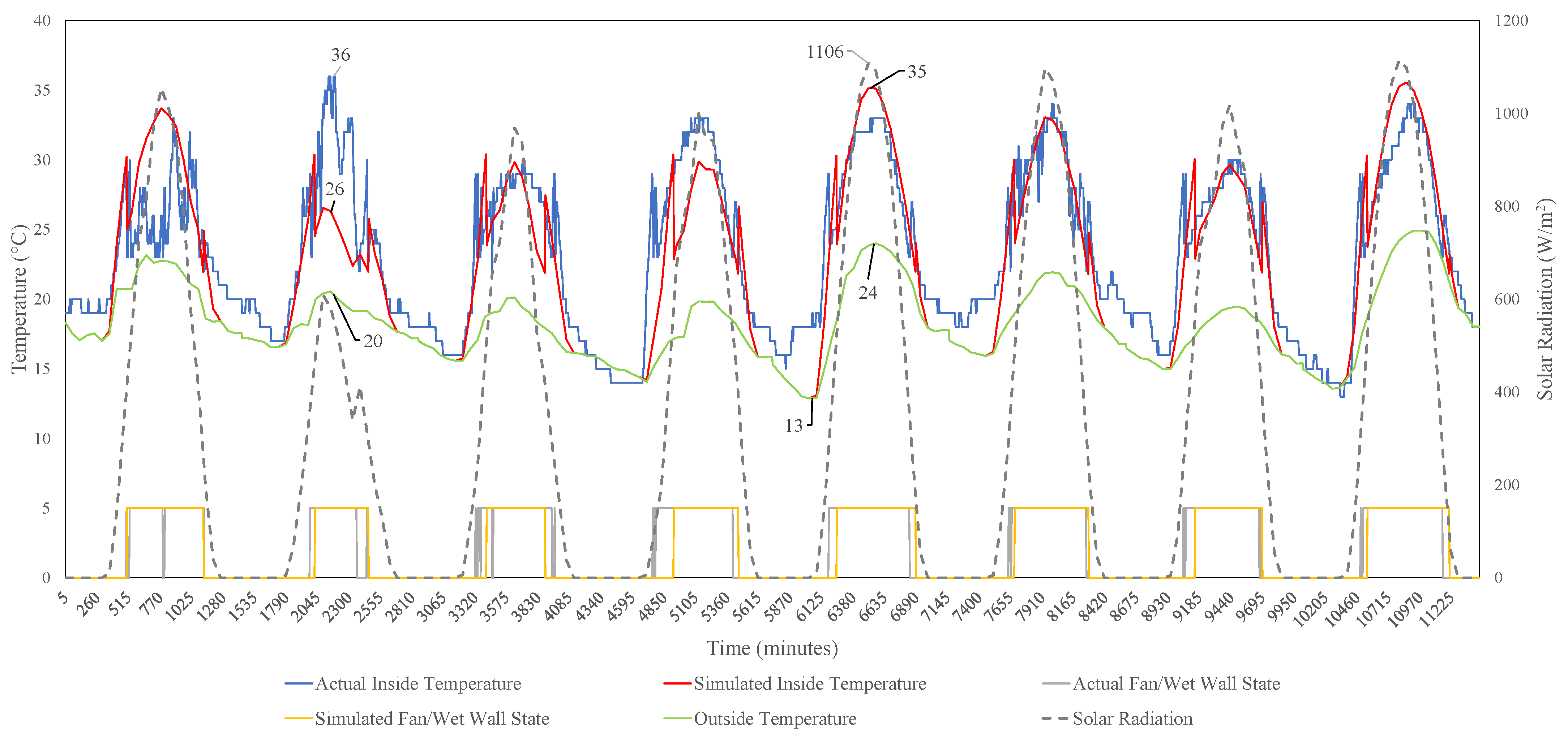
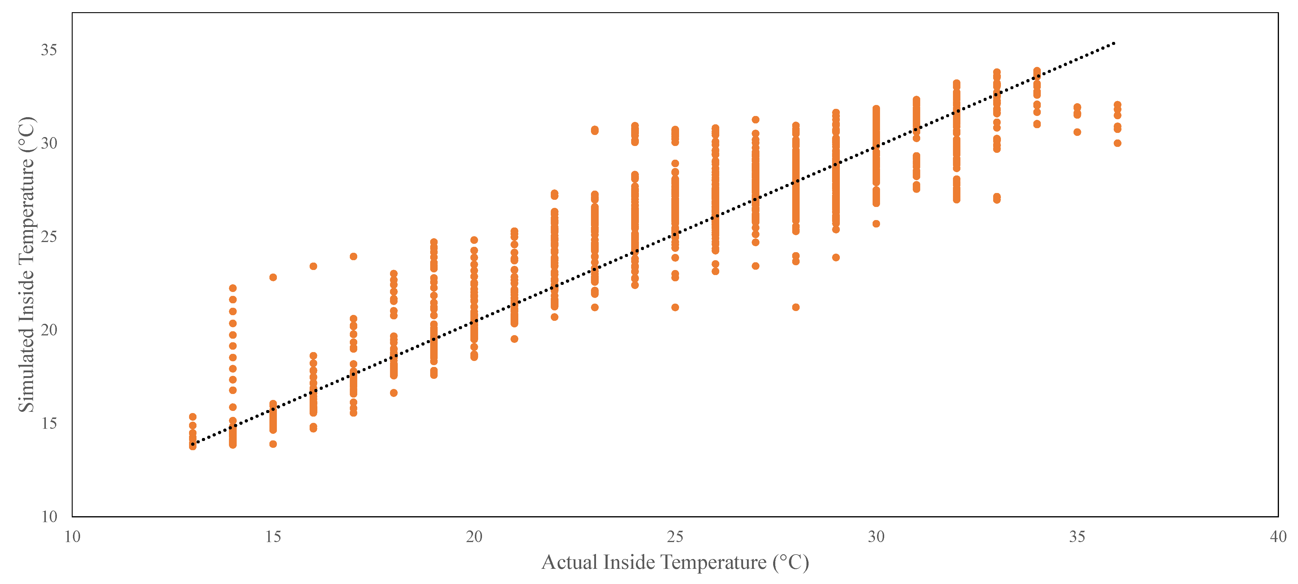
4.1. Analytical Model

Firstly, the results from the parameter optimisation were relatively close to what was expected. For V, the ventilation rate, the optimisation found 2 m³/s to be the best choice for the model, which is close to the 2.4 m³/s based on the fan’s advertised ventilation rate [42]. The heat loss coefficient (or thermal conductivity), $K_c$, was 3 W/m² °C, whereas the value used in Kittas et al. [41] was 4.2 W/m² °C. A slight difference was expected, however, as the type of covering used was different in both cases. The transmissivity of the greenhouse cover, $\tau$, was expected to be higher as the greenhouse’s internal temperatures are heavily influenced by solar radiation.

However, it seems that a large portion of the solar radiation energy is absorbed by the greenhouse cover or is reflected back into the surrounding air. The plant transpiration coefficient, $\alpha$, was much higher than Kittas et al. [41]. As we mentioned earlier, this may be due to the black aeroponics containers and the crops used in the trial inside the tunnel. Finally, $\eta$, the cooling efficiency of the wet wall, was unexpectedly 0.3 compared to the 0.8 that Kittas et al. [41] used. Again, this inefficiency may be due to the age of the wet wall.

The resultant analytical model in Figure 2 performs well but has significant errors in certain edge cases.

For the analytical model, the outside temperature and solar radiation significantly affect the model’s predictions, which can be seen where the predicted inside temperature is the same as the outside temperature at 13 °C. Further, on the second day in the test set, a large error of 10 °C occurs. This can be attributed to the model’s reliance on outside temperature and solar radiation, which is lower than expected for this day. As this weather station is not located at the farm, the conditions it experienced were vastly different to the tunnel, which is evident as the inside temperature reached 36 °C.

The predictive capabilities of the model are clear in Figure 3. The model’s simulated inside temperatures (on the y-axis) compared to the actual inside temperature (on the x-axis) is a way to confirm the model is predicting actual values rather than predicting random ones. A generally linear relationship is present, proving the predictions are not random. However, large variations are seen at high temperatures above about 24 °C. This is when the fan is predicted to turn on, which heavily influences the predictive accuracy of the model.

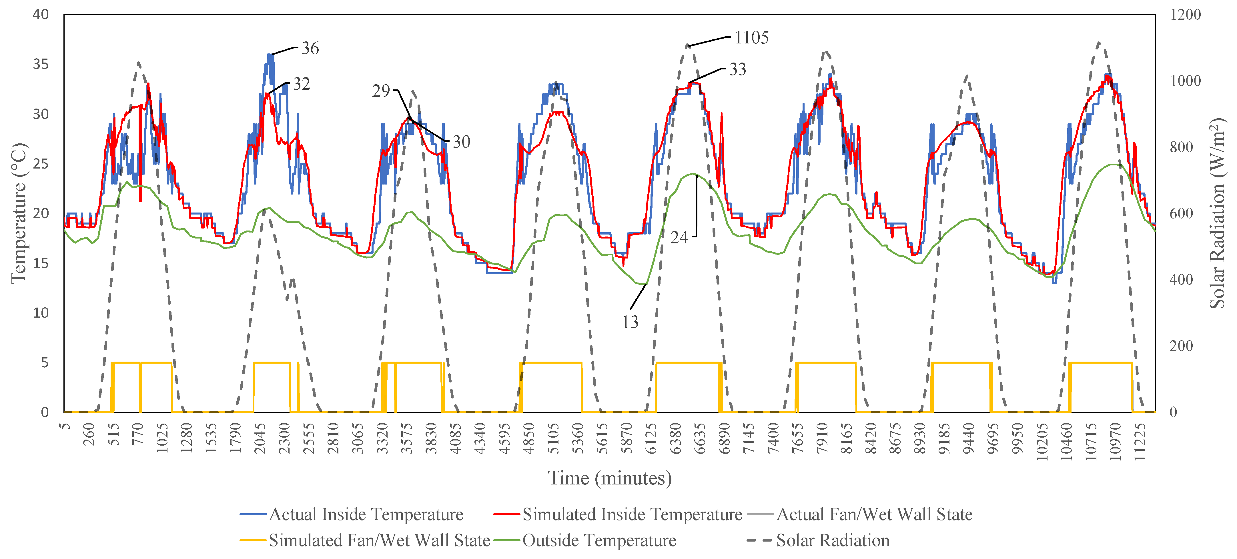
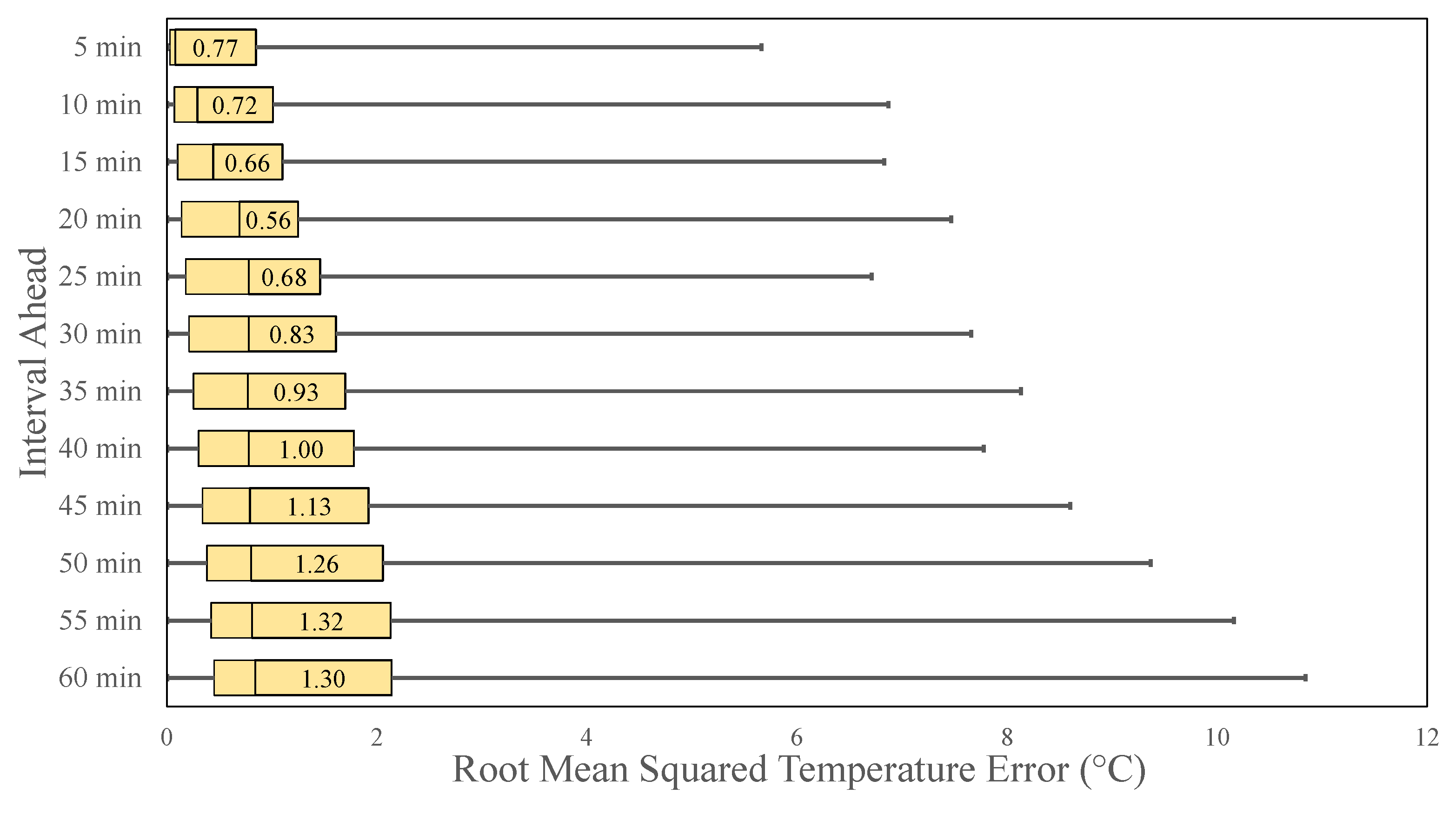
4.2. SVR Predictive Model

Figure 4 displays a one-hour-ahead simulation, demonstrating the method’s accuracy in predicting tunnel temperatures, despite occasional larger errors caused by abrupt temperature changes. The model effectively captures temperature variations, especially during rapid changes like shifts in cloud cover. Additionally, the model accurately simulates the fan and wet wall states based on predicted temperatures, showcasing its ability to account for these factors’ impact on internal temperatures.

Figure 5 substantiates the model’s credibility by illustrating a generally linear relationship between simulated and actual temperatures, dispelling concerns of random noise predictions. Despite a margin of error at higher temperatures, particularly during midday when cloud cover affects solar radiation, the model maintains overall accuracy.

Comparing Figure 3 and Figure 5 highlights the superior performance of the Support Vector Regression (SVR) model over the analytical model in terms of prediction accuracy. This outcome aligns with expectations, as the SVR model excels at capturing underlying patterns, overcoming limitations imposed by assumptions in the analytical model for computational ease.

Figure 6 shows the distribution of prediction errors in five minute increments. The results indicate significant errors, approaching approximately 12 °C for one-hour-ahead predictions. However, even for this forecast horizon, the median error is still 1.3 °C. When predicting for 15 min ahead, the error is 0.66 °C. This is smaller than the RMSE reported in

Table 2. Models’ performance.

Model Used	RMSE (°C)	MAE (°C)	MBE	${\mathit{R}}^2$
5 min ahead prediction	0.87	0.47	−0.05	0.98
30 min ahead simulation	1.31	0.86	−0.15	0.95
1 h ahead simulation	1.76	1.17	−0.24	0.9
Analytical model	2.93	2.16	−1.029	0.80

. In total, the incremental predictions integrate over the multiple estimations, thereby increasing the error for predictions further ahead.

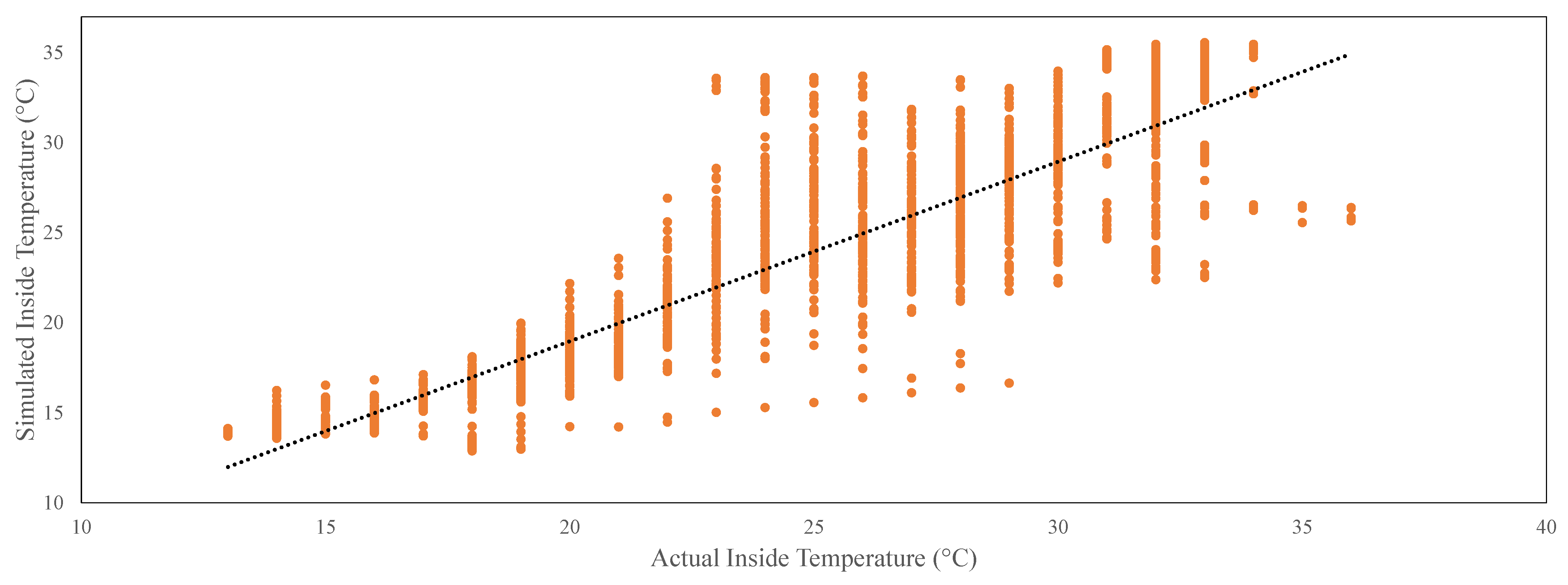
4.3. Model Performance

Table 2 quantifies the accuracies of the simulation process. The simulation becomes increasingly less accurate in its predictions from 5 min ahead to 1 h ahead. Regardless, the RMSEs for both 30 min and 1 h ahead are less than 1 °C more than the five-minute-ahead prediction. $R^2$ reduces from 0.98 to 0.9 for the three predictions. The model’s MAE accuracy is therefore slightly more than 1 °C for the case of predicting one hour ahead. Further, it is clear in Figure 5 that there is a wide variance in error for some predictions. This variation is largest at temperatures between when the fan and wet wall turn on or off. Because of the fan and wet wall’s effect on the internal temperatures of the greenhouse, the model is more likely to overpredict what the temperature is likely to be while simulating as it expects the temperature to continue to rise, but it is reduced by the fan and wet wall. This is clear at lower temperatures where the variation in the predicted temperatures is much lower than that at higher temperatures.

Compared to the empirical model, the analytical model is far less accurate in predicting the internal conditions of the tunnel. This may be due to the absence of the model accounting for time dependencies in the inside temperature, which leads to larger errors. Further, because this model is more dependent on solar radiation and the outside temperature, it leads to larger errors as seen in the RMSE value of 2.93 °C. In applications in different locations, the model does not need to be compensated to a large extent. Instead, the model requires hourly data to be interpolated into five minute intervals, or to use five minute intervals for the outside temperature data. Finally, it is less accurate when describing the data as seen by the $R^2$ value of 0.8. Despite the reduction in accuracy, this model does not require previous inside temperatures to predict the internal temperatures of the tunnel and can use forecasted data for the outside temperature and solar radiation. Further, it is possible to create a binary classifier based on the outside temperature and solar radiation to predict the fan/wet wall state. This means the analytical model can act independently from temporal data, which allows flexibility for a farmer to apply the outside temperature and solar radiation at any time of the day to see the internal temperatures of their greenhouse tunnel.

5. Discussion: Applications and Future Work

Based on the models developed in this study, real-time modelling of the temperature inside of the greenhouse tunnel is possible at an acceptable accuracy. By forecasting internal temperatures of the day using available weather services and measured data, predictive forecasting using the empirical model can occur to provide accurate feedback on the temperature of the greenhouse. Further, the analytical model can be used for an overall temperature profile of the greenhouse temperature for the entire day. Although the analytical model is not as accurate, it can give an insight for agriculturalists to plan and prepare for temperature variations within the tunnel, and use the model to plan what crops to grow. Using this forecasting method allows for improved preparedness in addressing the temperature variability associated with climate change and its impact on agriculture. This can aid in choosing the right plants and growing orientations for precision agriculture. The spatial resolution can be improved with an increased number of sensors dispersed throughout a tunnel to characterise the temperature biases that exist in a greenhouse tunnel. Moreover, it is crucial to explore the evident aspect of the relationship between plant life in the greenhouse and the climatic environment. To achieve this, a comprehensive study should be undertaken to investigate the impact of altering temperature ranges through fan and wet wall control on crop physiology. Future applications and developments of these models can include the introduction of neural networks and other computationally heavy models to edge devices within the greenhouse for improved real-time forecasting and prediction. Using such models can lead to advanced digital twins that can improve productivity and, potentially, even yield if used for decision making. Further, as discussed before, Fu and Zhou [28] used agricultural modelling to simulate energy consumption in a greenhouse. Although our work focused on the thermal modelling, we believe our models can be combined to develop a full digital twin solution that can provide different energy transfers in to and out of a greenhouse. For South African farmers, this could lead to fully self-sufficient greenhouses that only use renewable energy for agricultural production, promoting improved climate change resilience. Other work can focus on the economic viability of this solution and how it can affect self-sufficient farmers.

6. Conclusions

The objective of this study was to develop a smart digital twin solution to assist farmers in decision-making. The focus was on understanding thermodynamics and delivering predictive solutions to benefit farmers. This body of work can be adapted to provide similar digital twin solutions to Zhang et al. [27], excluding the electrical energy modelling.

The work conducted in this study represents a first step in thermal modelling of a greenhouse tunnel in the Stellenbosch area of South Africa. The tunnel, with its specific orientation, has been modelled in an empirical and analytical model that is capable of predicting the interior temperatures accurately.

Compared to Jogunola et al. [38], the RMSE for the SVR simulation process is significantly higher (1.76 °C vs. 0.025 °C). Due to the nature of the CNN and LSTM learning process, these models are able to learn sequences of time-dependent events better than the almost linear SVR process. This leads to better predictive capabilities and much more accurate modelling. However, the resolution of the data in Jogunola et al. [38] was hourly using either all or only one input feature. The disparity in RMSE is then justified as a higher resolution can introduce more errors into the model, especially when a prediction is fed back into the model to predict the following time. Further, the major trade-off in this accuracy is computation time for the neural network models compared to the simplistic nature of the SVR. For the analytical model, its RMSE is also significantly higher than that seen in Jogunola et al. [38], but this too is a much simpler and quicker modelling technique that requires a one-off parameter optimization for the different environmental variables.

When focusing on the analytical model, it is clear that it is accurate when compared to other literature, in particular, Nauta et al. [34] in which they achieved an RMSE of 4.25 °C. In Tong et al. [36], the authors used far more sensors and more cumbersome thermodynamic and heat transfer equations to produce an error of 1.0 °C at night and 1.5 °C during the day. Therefore, it is clear that although the models are not as accurate as the models developed in the literature, they have a low computational cost and simpler implementation of modelling techniques that can lead to similar results and a higher resolution of predictions that can aid in decision making in near real time. Having the capability to forecast tunnel temperatures one hour in advance allows farmers to enhance their readiness for unforeseen temperature changes. This, in turn, enables farmers to make more informed decisions regarding crop management within greenhouse tunnels. Additionally, this advancement contributes to an enhanced comprehension of thermodynamics within South African greenhouse tunnels, paving the way for improved physics-based modelling of African greenhouses in the times to come.

References

1. Mohamed, M.A.; El Afandi, G.S.; El-Mahdy, M.E.S. Impact of climate change on rainfall variability in the Blue Nile basin. Alex. Eng. J. 2022, 61, 3265–3275. [Google Scholar] [CrossRef]
2. Yang, H.; He, J.; Su, Y.; Xu, J. Adaptation to climate change: Ethnic groups in Southwest China. Environ. Hazards 2022, 21, 117–136. [Google Scholar] [CrossRef]
3. Eftekhari, M.S. Impacts of Climate Change on Agriculture and Horticulture. In Climate Change; Springer: Berlin/Heidelberg, Germany, 2022; pp. 117–131. [Google Scholar]
4. Wang, X.B.; Azarbad, H.; Leclerc, L.; Dozois, J.; Mukula, E.; Yergeau, É. A Drying-Rewetting Cycle Imposes More Important Shifts on Soil Microbial Communities than Does Reduced Precipitation. Msystems 2022, 7, e00247-22. [Google Scholar] [CrossRef] [PubMed]
5. Bopche, U.; Kingra, P.K.; Setia, R.; Singh, S.P. Spatio-temporal analysis of meteorological drought in Punjab under past, present and future climate change scenarios. Arab. J. Geosci. 2022, 15, 756. [Google Scholar] [CrossRef]
6. Ahmad, M.M.; Yaseen, M.; Saqib, S.E. Climate change impacts of drought on the livelihood of dryland smallholders: Implications of adaptation challenges. Int. J. Disaster Risk Reduct. 2022, 80, 103210. [Google Scholar] [CrossRef]
7. Fujimori, S.; Wu, W.; Doelman, J.; Frank, S.; Hristov, J.; Kyle, P.; Sands, R.; Van Zeist, W.J.; Havlik, P.; Domínguez, I.P.; et al. Land-based climate change mitigation measures can affect agricultural markets and food security. Nat. Food 2022, 3, 110–121. [Google Scholar] [CrossRef] [PubMed]
8. Munaweera, T.; Jayawardana, N.; Rajaratnam, R.; Dissanayake, N. Modern plant biotechnology as a strategy in addressing climate change and attaining food security. Agric. Food Secur. 2022, 11, 26. [Google Scholar] [CrossRef]
9. Wang, H.; Xu, C.; Liu, Y.; Jeppesen, E.; Svenning, J.C.; Wu, J.; Zhang, W.; Zhou, T.; Wang, P.; Nangombe, S.; et al. From unusual suspect to serial killer: Cyanotoxins boosted by climate change may jeopardize megafauna. Innovation 2021, 2, 100092. [Google Scholar] [CrossRef] [PubMed]
10. Ruggerio, C.A. Sustainability and sustainable development: A review of principles and definitions. Sci. Total Environ. 2021, 786, 147481. [Google Scholar] [CrossRef] [PubMed]
11. Abbass, K.; Qasim, M.Z.; Song, H.; Murshed, M.; Mahmood, H.; Younis, I. A review of the global climate change impacts, adaptation, and sustainable mitigation measures. Environ. Sci. Pollut. Res. 2022, 29, 42539–42559. [Google Scholar] [CrossRef]
12. Waaswa, A.; Oywaya Nkurumwa, A.; Mwangi Kibe, A.; Ngeno Kipkemoi, J. Climate-Smart agriculture and potato production in Kenya: Review of the determinants of practice. Clim. Dev. 2022, 14, 75–90. [Google Scholar] [CrossRef]
13. Ogunyiola, A.; Gardezi, M.; Vij, S. Smallholder farmers’ engagement with climate smart agriculture in Africa: Role of local knowledge and upscaling. Clim. Policy 2022, 22, 411–426. [Google Scholar] [CrossRef]
14. von Braun, J. Food insecurity, hunger and malnutrition: Necessary policy and technology changes. New Biotechnol. 2010, 27, 449–452. [Google Scholar] [CrossRef]
15. Anderson, M.D.; Rivera Ferre, M.G. Unsustainable by design: Extractive narratives of ending hunger and regenerative alternatives. Curr. Opin. Environ. Sustain. 2020. [Google Scholar] [CrossRef]
16. Benke, K.; Tomkins, B. Future food-production systems: Vertical farming and controlled-environment agriculture. Sustain. Sci. Pract. Policy 2017, 13, 13–26. [Google Scholar] [CrossRef]
17. Puri-Mirza, A. UAE: Abu Dhabi Contribution of Agriculture, Forestry and Fishing to the GDP 2019. 2021. Available online: https://www.statista.com/statistics/818124/uae-contribution-of-agriculture-forestry-and-fishing-to-the-gdp-in-abu-dhabi/ (accessed on 17 November 2023).
18. Shafi, U.; Mumtaz, R.; García-Nieto, J.; Hassan, S.A.; Zaidi, S.A.R.; Iqbal, N. Precision agriculture techniques and practices: From considerations to applications. Sensors 2019, 19, 3796. [Google Scholar] [CrossRef]
19. Lowenberg-DeBoer, J.; Erickson, B. Setting the record straight on precision agriculture adoption. Agron. J. 2019, 111, 1552–1569. [Google Scholar] [CrossRef]
20. Montzka, S.A.; Dlugokencky, E.J.; Butler, J.H. Non-CO2 greenhouse gases and climate change. Nature 2011, 476, 43–50. [Google Scholar] [CrossRef]
21. Balafoutis, A.; Beck, B.; Fountas, S.; Vangeyte, J.; Van der Wal, T.; Soto, I.; Gómez-Barbero, M.; Barnes, A.; Eory, V. Precision agriculture technologies positively contributing to GHG emissions mitigation, farm productivity and economics. Sustainability 2017, 9, 1339. [Google Scholar] [CrossRef]
22. Mabitsela, M.M.; Motsi, H.; Hull, K.J.; Labuschagne, D.P.; Booysen, M.J.; Mavengahama, S.; Phiri, E.E. First report of aeroponically grown Bambara groundnut, an African indigenous hypogeal legume: Implications for climate adaptation. Heliyon 2023, 9. [Google Scholar] [CrossRef]
23. Mizik, T. Climate-smart agriculture on small-scale farms: A systematic literature review. Agronomy 2021, 11, 1096. [Google Scholar] [CrossRef]
24. Doyle, L.; Oliver, L.; Whitworth, C. Design of a climate smart farming system in East Africa. In Proceedings of the 2018 IEEE Global Humanitarian Technology Conference (GHTC), San Jose, CA, USA, 18–21 October 2018; pp. 1–6. [Google Scholar]
25. Atayero, A.A.; Oluwatobi, S.; Alege, P.O. An assessment of the Internet of Things (IoT) adoption readiness of Sub-Saharan Africa. J. S. Afr. Bus. Res. 2016, 13, 1–13. [Google Scholar] [CrossRef]
26. Nigussie, E.; Olwal, T.; Musumba, G.; Tegegne, T.; Lemma, A.; Mekuria, F. IoT-based irrigation management for smallholder farmers in rural sub-Saharan Africa. Procedia Comput. Sci. 2020, 177, 86–93. [Google Scholar] [CrossRef]
27. Zhang, X.; Fu, X.; Xue, Y.; Chang, X.; Bai, X. A review on basic theory and technology of agricultural energy internet. IET Renew. Power Gener. 2023. Available online: https://ietresearch.onlinelibrary.wiley.com/doi/pdf/10.1049/rpg2.12808 (accessed on 15 January 2024).
28. Fu, X.; Zhou, Y. Collaborative Optimization of PV Greenhouses and Clean Energy Systems in Rural Areas. IEEE Trans. Sustain. Energy 2023, 14, 642–656. [Google Scholar] [CrossRef]
29. Jans-Singh, M.; Leeming, K.; Choudhary, R.; Girolami, M. Digital twin of an urban-integrated hydroponic farm. Data-Centric Eng. 2020, 1, e20. [Google Scholar] [CrossRef]
30. Patil, S.; Tantau, H.; Salokhe, V. Modelling of tropical greenhouse temperature by auto regressive and neural network models. Biosyst. Eng. 2008, 99, 423–431. [Google Scholar] [CrossRef]
31. Allouhi, A.; Choab, N.; Hamrani, A.; Saadeddine, S. Machine learning algorithms to assess the thermal behavior of a Moroccan agriculture greenhouse. Clean. Eng. Technol. 2021, 5, 100346. [Google Scholar] [CrossRef]
32. Aissa, M.; Boutelhig, A. CFD Comparative Study between Different Forms of Solar Greenhouses and Orientation Effect. Int. J. Heat Technol. 2021, 39, 433–440. [Google Scholar] [CrossRef]
33. Mobtaker, H.G.; Ajabshirchi, Y.; Ranjbar, S.F.; Matloobi, M. Simulation of thermal performance of solar greenhouse in north-west of Iran: An experimental validation. Renew. Energy 2019, 135, 88–97. [Google Scholar] [CrossRef]
34. Nauta, A.; Lubitz, W.D.; Tasnim, S.; Mahmud, S. Thermal modelling of greenhouse using 1D lumped capacitance model. In Proceedings of the 5th International Conference of the International Commission of Agricultural and Biosystems Engineering, Quebec, BC, Canada, 10–14 May 2021. [Google Scholar]
35. Tadj, N.; Draoui, B.; Theodoridis, G.; Bartzanas, T.; Kittas, C. Convective heat transfer in a heated greenhouse tunnel. In Proceedings of the VIII International Symposium on Protected Cultivation in Mild Winter Climates: Advances in Soil and Soilless Cultivation under 747; Acta Horticulture: Agadir, Morocco, 2006; pp. 113–120. [Google Scholar]
36. Tong, G.; Christopher, D.; Li, B. Numerical modelling of temperature variations in a Chinese solar greenhouse. Comput. Electron. Agric. 2009, 68, 129–139. [Google Scholar] [CrossRef]
37. Tacarindua, C.R.; Shiraiwa, T.; Homma, K.; Kumagai, E.; Sameshima, R. The effects of increased temperature on crop growth and yield of soybean grown in a temperature gradient chamber. Field Crop. Res. 2013, 154, 74–81. [Google Scholar] [CrossRef]
38. Jogunola, O.; Hull, K.; Mabitsela, M.; Phiri, E.E.; Booysen, M.J. Deep Learning-Enabled Temperature Simulation of a Greenhouse Tunnel. 2023. Available online: https://www.researchgate.net/publication/377265253_Deep_Learning-Enabled_Temperature_Simulation_of_a_Greenhouse_Tunnel (accessed on 15 January 2024).
39. Hull, K.; Mabitsela, M.; Phiri, E.; Booysen, M. Dataset of temperature, humidity, and actuator states of an east-facing South African Greenhouse Tunnel. Data Brief 2023, 51, 109633. [Google Scholar] [CrossRef] [PubMed]
40. Kittas, C.; Bartzanas, T.; Jaffrin, A. Greenhouse evaporative cooling: Measurement and data analysis. Trans. ASAE 2001, 44, 683. [Google Scholar] [CrossRef]
41. Kittas, C.; Bartzanas, T.; Jaffrin, A. Temperature gradients in a partially shaded large greenhouse equipped with evaporative cooling pads. Biosyst. Eng. 2003, 85, 87–94. [Google Scholar] [CrossRef]
42. CFWFans. Maxiflow Fans. Available online: https://www.cfwfans.co.za/wp-content/uploads/2019/07/Maxiflow-Brochure.pdf (accessed on 10 August 2023).
43. Meteoblue. Universität Basel, Basel, Switzerland. Available online: https://www.meteoblue.com (accessed on 15 August 2023).
44. Hull, K.; Mabitsela, M.; Phiri, E.E.; Booysen, M. Temperature and Humidity Dataset of an East-Facing South African Greenhouse Tunnel. Mendeley Data 2024, V2. [Google Scholar] [CrossRef]
45. Hull, K.; Booysen, M.; Mabitsela, M.; Phiri, E.E. Using a Digital Twin for Greenhouse Tunnel Temperature Management and Prediction. In Proceedings of the 2023 IEEE AFRICON, Nairobi, Kenya, 20–22 September 2023; pp. 1–6. [Google Scholar] [CrossRef]
Figure 1. The tunnel is arranged as shown in these figures, with the placement of each temperature and humidity sensor shown in relation to the climate control (comprising a fan and wet wall). (a) The tunnel is approximately 28 m in length and has a wet wall on the one end, and an extraction fan on opposite ends, with no other openings. (b) Tunnel layout with sensor positions [39].
Agriengineering 06 00017 g001
Figure 2. Analytical model (in red) compared to the actual temperature (in blue). Replicated with permission from [45].
Agriengineering 06 00017 g002
Figure 3. The trend (dotted black line) shows a linear relationship between the actual temperatures and the analytical model’s temperatures (orange dots); however, this relationship has an R2 value of 0.8, which is clear with the larger variances in simulated temperatures, compared to the actual observed temperatures. Replicated with permission from [45].
Agriengineering 06 00017 g003
Figure 4. Data-driven model. The model closely follows the measured temperatures. However, the simulated fan does not always turn on at lower temperatures.
Agriengineering 06 00017 g004
Figure 5. Relationship between the simulated measured and predicted temperatures. The trend (dotted black line) shows a linear relationship between the actual temperatures and the model’s temperatures (orange dots) An R2 value of 0.9 was achieved with the SVR model and the correlation is clear between the observed and simulated data.
Agriengineering 06 00017 g005
Figure 6. The prediction errors for incremental prediction horizons, illustrating the increasing simulation errors.
Agriengineering 06 00017 g006