Digital Mapping of Topsoil Texture Classes Using a Hybridized Classical Statistics–Artificial Neural Networks Approach and Relief Data

Abstract

The demand for high quality and low-cost spatial distribution information of soil texture classes (STCs) is of great necessity in developing countries. This paper explored digital mapping of topsoil STCs using soil fractions, terrain attributes and artificial neural network (ANN) algorithms. The 4493 soil samples covering 10 out of 12 STCs were collected from the rice fields of the Guilan Province of Northern Iran. Nearly 75% of the dataset was used to train the ANN algorithm and the remaining 25% to apply a repeated 10-fold cross-validation. Spatial prediction of soil texture fractions was carried out via geostatistics and then a pixel-based approach with an ANN algorithm was performed to predict STCs. The ANN presented reasonable accuracy in estimating USDA STCs with a kappa coefficient of 0.38 and pixel classification accuracy percentage of 52%. Hybridizing soil particles with relief covariates yielded better estimates for coarse- and medium-STCs. The results also showed that clay particle and terrain attributes are more important covariates than plant indices in areas under single crop cultivation. However, it is recommended to examine the approach in areas with diverse vegetation cover.

1. Introduction

Detailed high-resolution soil property maps are an essential tool for agricultural management and environmental sustainability [1], including management zones in precision agriculture [2], land management, civil projects, and environmental risk assessment [3,4,5]. Soil texture is one of the main characteristics that controls buffering capacity [6], nutrient availability [7,8], carbon cycle [9,10] and diagnostic horizon characteristics of soil taxonomy [11] as well as erodibility and water dynamics [12]. Soil texture is a relatively stable property over time, which makes it a useful measure for predicting spatially distributed nonuniformity of soil [13]. It is the most frequently used input for PedoTransfer functions (PTFs) in predicting different soil characteristics [14]. Since soil texture often has considerable variability both laterally and vertically [15] due to geologic and pedogenic processes, for soil scientists, producing such information is a key challenge in land use planning, soil protection measurements and soil moisture regime [16,17] at different spatiotemporal resolutions [18,19], especially in Iran [20,21,22].

Soil textural classes are generally estimated via two main direct (point source) and indirect (by model) approaches. In the latter, soil texture fractions (STFs) are incorporated with environmental variables to spatially estimate soil texture classes [23]. Although laboratory STF measurement for soil texture classification is not very costly, determining and understanding its behavior is a challenge due to the high sampling costs and time consumption [24,25]. Conventional statistics are unable to discriminate between various sources of spatial variability influencing soil properties in a surveyed site. This is because their relationships are blurred and different variations are mixed in the classical approach [26]. However, geostatistics examine both the spatial distribution and dependency of the attributed values. Although soil scientists believe in soil variation at different scales, knowledge of changes in soil properties is still limited [19]. To overcome this challenge, authors of [25,27] proposed digital soil texture mapping based on spatial prediction methods such as geostatistics and multinomial logistic regression (MLR) coupled with remote sensing. Despite the results of [28] showing similar accuracies in predicting STFs for both untransformed and transformed datasets, authors of [29] reported that STF transformation resulted in better estimates.

The qualitative variables were rarely investigated by soil scientists both at local and regional scales, specifically in forest, hillslope, desert and mountainous land uses, which have broadly been ignored in recent studies in Iran [22]. For instance, Zaeri et al. [30] stated that interpolating qualitative data by using traditional geostatistical techniques is difficult, as these methods were generally focused on describing and predicting numerical variables. Contrary to quantitative data, the qualitative data could not be estimated by observing neighboring observations of linear methods. At national level, Paterson et al. [19] modeled the spatial variability of soil texture in Australia using the country’s legacy data set (National Soil Site Collation, NSSC) at 1 km to continental scales. They used a grid-based declustering method and an experimental variogram using spatial declustering to manage the challenges. Hengl et al. [31] mapped Iran’s soil textural classes using four interpolators. Based on the results, they introduced regression kriging as the optimal method for mapping.

Widelyused SCORPAN is a basis of DSM, which makes relationships between soil attributes or classes and other spatially referenced factors [32]. The SCORPAN model by McBratney et al. [33] offers an authentic approach to spatial prediction of soil attribute classes [32] using auxiliary data. Among environmental factors, terrain attributes represent the relief in the SCORPAN equation of [33]. Zhang et al. [34] indicated that if auxiliary variables were appropriately selected, it would be possible to satisfactorily estimate soil texture. It seems that the spatial modelling of the soil texture class is highly dependent on the situation of the study area, i.e., the soil texture classes showed different correlation with different covariates at different areas. For example, Zhou et al. [1] found good results from using RS-based plant indices to predict soil texture classes because the studied area had a diverse vegetation cover as a result of subtropical climate. Thus, plant indices have strongly entered the modelling of soil texture classes. However, Kaya and Başayiğit [27] found reasonable accuracy mainly using terrain attributes due to high elevation and physiographic feature diversity in the studied area.

According to Padarian et al. [35], various widespread machine learning (MS)-based techniques including ANN, deep learning (DL), fuzzy, boosted regression trees (BRT) and random forest (RF) have been studied by many researches due to their accuracy and adaptability capabilities, ability to capture nonlinear relationships [1,5,14,28,36,37,38,39,40,41,42]. It seems that model performance is site-specifically changed and dissimilar outputs are acquired when provided the same inputs [43]. Moreover, advanced ML methods usually perform better than simpler ones [35]. For example, Taghizadeh-Mehrjardi et al. [14] and Yang et al. [44] proved that convolutional neural networks (CNNs) outperform RF since CNNs are able to integrate contextual information about the landscape, which is of great help in DSM analysis. An interpretable machine learning (ML) strategy, namely the Shapley additive explanations (SHAP) method has recently been proposed by Zhou et al. [1], which enables the improvement of the transparency in black-box ML models. Pixel-based classification is one of the most powerful methods of producing qualitative thematic maps derived from aquantitative classification approach that uses various spectral bands, data extracted from the digital elevation model (DEM) and/or soil forming factors. This method entails assigning each pixel to a specific class. The pixel-based method has rarely been used for evaluating soil properties, and the few conducted have mostly focused on biophysical properties [45,46,47,48]. An ANN is an alternative to pixel-based methods with assumption constraints such as normality, linearity and variable independence. It can also extract patterns and recognize trends in complex and uncertain data [49]. Moreover, it was widely used in hydrology and pedology for mapping purposes due to its capability of describing nonlinear relationships [50,51,52,53,54]. ANNs have historically been combined with geostatistical methods in hydrological studies for spatial distribution of variables, e.g., soil organic matter, salinity, soil water content and total N, but they have recently been employed for mapping soil properties [55,56,57].

A review of the past studies shows a lack of sufficient knowledge on the application of hybridized classical statistics and an ANN approach using remote sensing and STFs for spatial estimation of soil texture classes at the regional scale and under single crop cultivation. In addition, the study area included a wide range of soil texture classes, which is unique. Therefore, structural correlation for multivariate data characterization is required to analyze using geostatistics techniques. Additionally, most agricultural areas in Guilan Province are under rice cultivation, where the soil is puddled to improve water-holding capacity and control weeds, and the precise soil texture class map can lead to better land management. Therefore, integrating quantitative physical soil properties such as soil texture fractions (STFs) with environmental auxiliary data would increase the accuracy of soil texture class predictions. Consequently, this study aims to perform a digital soil mapping of topsoil texture classes with 30 m spatial resolution using remotely sensed data and STFs using ANN algorithms for a large geographical extension in Iran.

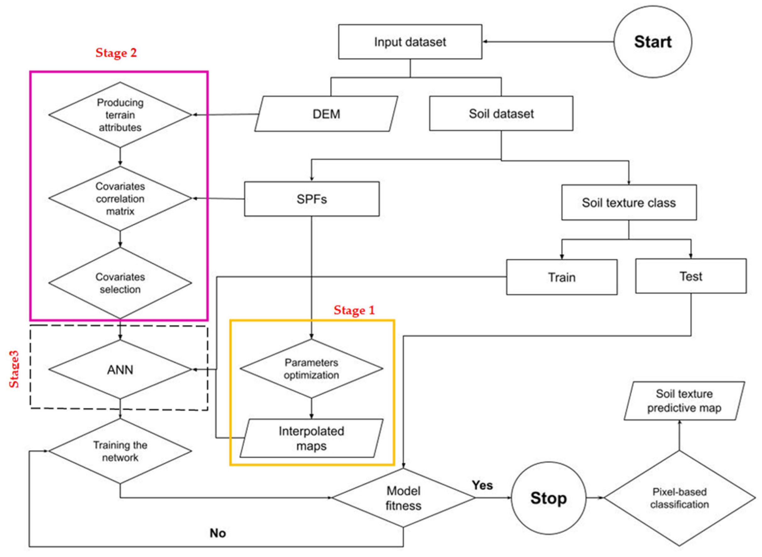
2. Materials and Methods

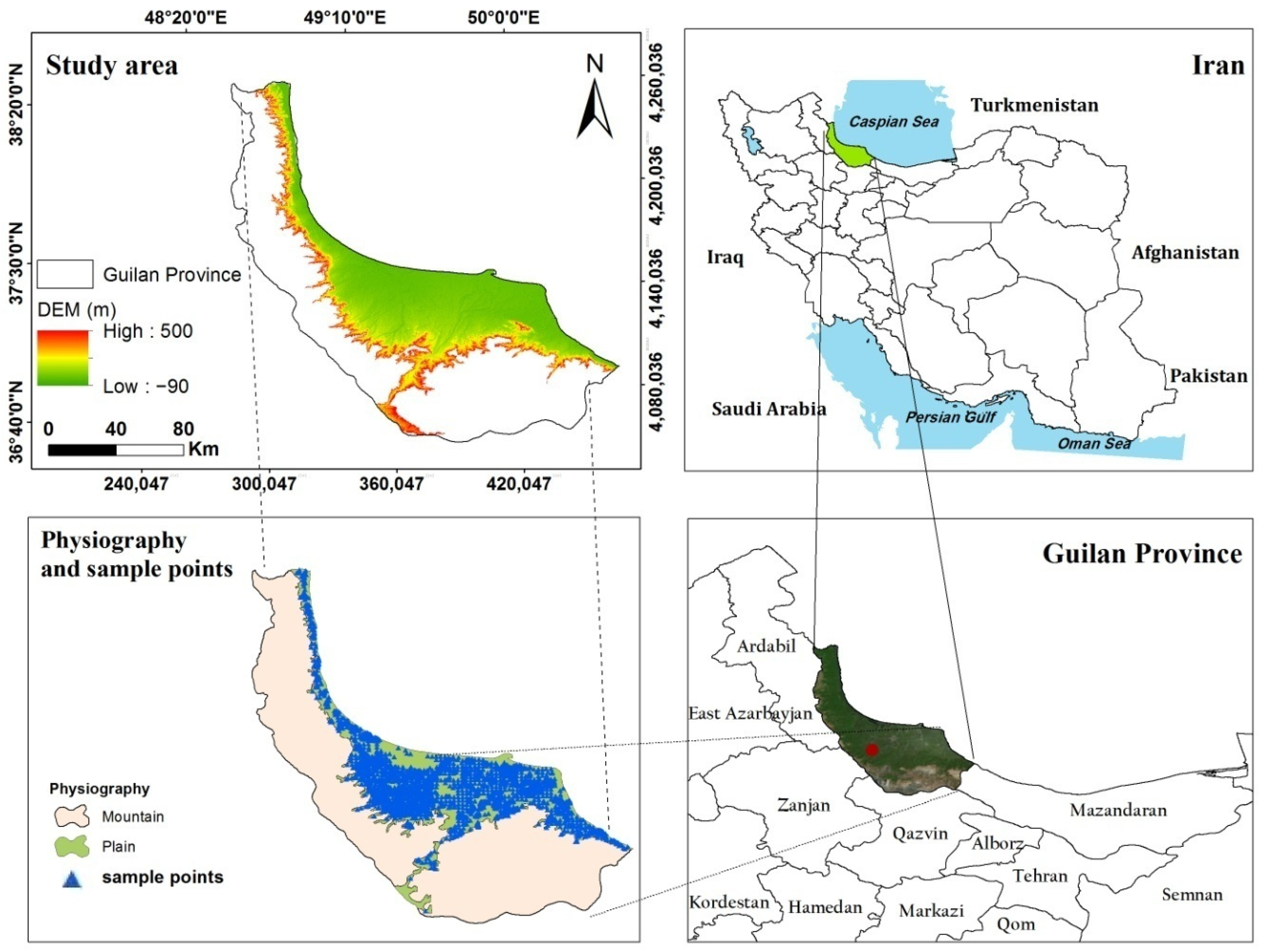
The model architecture and its detailed configuration are illustrated in Figure 1.

The approach consists of three main stages including (1) most probable STF-interpolated mapping, (2) covariate reduction and selection and (3) hybridization of STFs and selected covariates through ANN to predict soil texture class.

2.1. Study Area

The study area covers nearly 14,000 km² of the Guilan province in northern Iran (Figure 2), bordering the Caspian Sea to the north, Qazvin and Zanjan provinces to the south, Ardabil Province to the west and Mazandaran Province to the east. The elevation ranges from −90 m in the coastal zones to 660 m in the southern Alborz mountain chains. According to the deMartonne climate classification [58], Guilan’s northern and central regions have a very humid, temperate and warm Mediterranean climate whereas its southern regions have a cold, subhumid climate. Maximum precipitation occurs in Amlash with approximately 2270 mm, while annual average rainfall of Guilan province is 1260 mm. Hence, the soil moisture regime is udic, ustic and xeric along the same geographic gradient [59]. The irrigated and rainfed areas are 476,000 and 142,000 hectares, respectively. The rice fields are mostly located on low coastal alluvial plains on the mountainsides and alluvial fans. The main physiographic features are mountains (65.42%) and plains (34.58%). The rock-type geology of the agricultural lands matched with soil sample points were sedimentary (97.8%), igneous (1.6%), volcano-sedimentary (0.4%) and metamorphic (0.2%), respectively [60], which implies uniformity of the earth within the region of interest. The soils of agricultural areas are predominantly fertile as a result of favorable climatic conditions and play a key role in food security in Iran.

2.2. Soil Data

A quantity of 4870 soil samples were collected from different soil surveys at points located in different soil types based on legacy soil databank (Figure 2). These projects were conducted mainly on rice croplands between 2001 and 2018 by a joint project between the Rice Research Institute of Iran (RRII) and the Soil and Water Research Institute (SWRI), with the collaboration of private soil laboratories of Guilan Province and a number of MSc dissertations and PhD theses [61]. The dataset included clay, silt and sand content at 0–10, 0–15, 0–30 and 30–45 cm (rooting) depths. Three hundred and seventy-seven soil samples that presented incorrect spatial location or over outcrop, duplicates, outliers and the sum of the soil fractions exceeding 100% were excluded from the dataset. The remaining 4493 soil samples were normalized according to skewness and kurtosis.

Soil samples were air-dried, grounded and sieved to a 2 mm mesh. The hydrometer method [62] was used for measuring the soil particles percentage of all samples. Soil samples were classified in textural classes using USDA methods [62] implemented in the “NAME” package [63].

2.3. Parameter Optimization of STF Spatial Interpolation

The STFs must be evaluated with respect to centrality, distribution, outliers and normality of frequency distribution prior to geostatistical analysis. The centrality statistics were computed for each STF in Statistical Package for the Social Sciences (SPSS) software v.17 with the assumption that the data are spatially independent. The significance of skewness and kurtosis were used to test the normality of variable frequency distribution. The outliers were explored using the Norfolk test. Variables with nonnormal distributions were normalized using logarithmic transformations. Log-ratio transformations guarantee the effect of non summing of to 100% of STFs [28].

Geostatistics has been widely used to interpret the spatial variation of natural phenomena [64] as well as spatial variation of soil properties [65]. GS+ 9.1 [66] was conducted to build semi-variograms and analyze spatial structure of STFs. The semi-variogram is estimated using the following equation, presented by [67].

$$\left(h\right)=\frac{1}{2N\left(h\right)}{{\displaystyle \sum }}_{i=1}^{N\left(h\right)}{[Z\left(x_i\right)-Z\left(x_i+h\right)]}^2$$

(1)

where γ (h) is the semi variance, Z is the regionalized variable, Z (x_i) refers to the measured sample at point x_i, Z (x_i + h) is the measured sample at point (x_i + h) and N (h) is the number of pairs separated by distance or lag h.

The detailed spatial structure of STFs were investigated in the previous study [29] using semi-variogram models (spherical, exponential and linear). Selection of semi-variogram models was made according to the highest coefficient of determination (R²) and the smallest residual sum of squares (RSS) to fit the model. Variable isotropy was determined in various orientations using component analysis of the semi-variogram (the range, A₀; the sill, C + C₀; and the nugget, C₀) through linear, spherical, Gaussian and exponential methods with a nugget effect to verify the spatial applicability of the geostatistics. The nugget-to-sill ratio was used to quantify each variable’s strength of spatial dependence. This ratio represents the contribution of variance of the total variance. If the ratio is smaller than 25%, the spatial dependency is strong, if it is between 25 and 75%, the spatial dependence is moderate, and if it is above 75%, the spatial dependence is weak, according to [67].

The best-fitted model was then used in an ordinary kriging (OK) procedure considering transformation and back-transformation to clay, silt and sand values to estimate different STFs at unvisited points as interpolated values for mapping. The selected values were then employed to produce individual STF maps.

2.4. STF Interpolation

Two methods were used for interpolating STFs, namely (a) ordinary kriging (OK) and (b) inverse distance weighted (IDW) interpolations. The components of the models with sills were used for interpolating and representing variables using OK and IDW in ArcGIS 10.4.

In OK, the weighted average of data values in points neighboring an unvisited point was determined while considering the spatial structure of data based on the spatial correlation of the points [26]. Samples in the search radius were selected as the nearest neighbors by comparing the outcome of 5 to 25 points in the OK search radius using the evaluation statistics (results not shown). In the end, 20 were selected as the optimal number of neighboring points.

Inverse distance weighting (IDW) is one of the most extensively used practical interpolation methods, based on the hypothesis that the target variable value in the unvisited point is the weighted average of values in which weight decreases with distance from the function point [68]. In IDW, the choice of exponent value and number of nearest neighbors significantly affect estimation quality [69,70]. The estimations were performed in ArcGIS 10.4 by comparing 8 to 30 nearest points, and the estimated value was in the 1–4 range [69]; eventually, maps of all covariates were resampled to 30 × 30 m.

2.5. Covariate Selection

In DSM, covariates are generally derived from soil maps, DEM, remote sensing data and expert knowledge [33]. Here, RS-based auxiliary data were not used for predicting soil texture classes for the reason that they had a smaller contribution compared to other SCORPAN factors in a number of reviewed studies, specifically [38]. As can be seen in

Table 1. Literature review on the use of covariates for soil texture fractions and soil texture class estimations.

Reference	Variables		Strongest Correlation	Climate/Soil Moisture Regime	Scale/Location
	Dependent	Independent
Zhao et al., 2009 [42]	STFs: Sand; Clay.	The hydrographic parameters derived from DEM; SD; SDR; VSP.	Hydrographic parameters derived from DEM.	Average annual rainfall, snowfall, and daily temperatures are 730.7 mm, 306.7 cm and 3.7 °C, respectively.	Watershed, Canada
Greve et al., 2012 [36]	STFs: Coarse sand; Fine sand; Silt; Clay.	Seven primary terrain parameters: ELV; Slope gradient; Slope aspect. Existing maps: parent materials, landscape types, geographic region, profile curvature. Available pluviometric station data: yearlyprecipitation, seasonalprecipitation. CTI-extracted, generated usingLIDAR. Others: plan curvature, flow direction, flow accumulation.	Coarse sand: elevation (13%); fine sand: slope aspect (14%), ELV (12%), CTI (9%). Common in all STFs: parent materials (47–100%), geographic regions (31–100%) and landscape types (68–100%). Clay: Yearly-precipitation, Seasonal-precipitation, ELV (10%) Silt: Yearlyprecipitation, Seasonalprecipitation, parent materials (47% and 100%), geographic regions (31–100%), landscape types (68–100%).	Temperate climate with a mean winter temperature of 0 °C and a summer mean of 16 °C.	Denmark
Bakker A., 2012 [3]	STFs: Sand; Silt; Clay.	PC3; NDVI; DEM; Slope; TWI; CURVATURE; Profile; Planform; Temperature; Seasonal precipitation; SWI; CI; MI; QI.	STFs: Clay: temperature, seasonal precipitation, DEM, QI; Silt: seasonal precipitation, SLOPE, planform, CURVATURE, MI, NDVI; Sand: seasonal precipitation, NDVI, DEM, planform;	Warm, temperate with dry and hot summer.	Morocco
	ST		Slope; CURVATURE; Mineral indices; ASTER SWIR bands; ASTER TIR bands.
Liao et al., 2013 [24]	STFs: Sand; Silt; Clay.	Six bands DN of Landsat ETM: Bands 1–5 and Band 7; DN of Band 7.	Band 7 ETM
Wang et al., 2015 [25]	STFs: Sand; Clay; Physical clay content.	LSDT; LSNT; DTR. (During 2004, 2007 and 2008)	DTR	Not reported.	Farmland/ river plain, East China
Song et al., 2016 [39]	STFs: Sand; Clay.	ELV; TWI; Slope; ASP. Plan curvature; Profile curvature; MAP; MAAT; SR; NDVI; Land cover; ST.	Sand: DEM, MAAT, TWI, slope, SR, plan curvature, land cover. Clay: NDVI, ST, MAP, TWI, profile curvature.	Humid and cold.	Mountains/ Qinghai-Tibetan plateau, China, covered primarily by alpine meadow
Wu et al., 2018 [41]	STC: Sandy; Loamy; Clayey.	ELV; TCI_Low; Flow-PathL.	ELV; TCI_Low; Flow- PathLength.	MAP: 1037.7 mm.	Small mountainous watershed located in the core areas of a river in southwest China
Mehrabi-Gohari et al., 2019 [38]	STFs: Sand; Silt; Clay.	Terrain attributes extracted from DEM—90 m resolution (Slope, ASP, TWI, NDVI, etc.) B2, B3, B4, B5, B6, B7, B8, B10 and B11 Landsat 8 bands. Soil spectral data;	Soil spectral data. Spectrometric data; multi-resolution, valley-bottom flatness index and wetness index.	Arid.	Approximately 70 km awayfrom Kerman, city of Zarand, southeastern Iran
Amrian-Chakan et al., 2019 [28]	STFs: Sand; Silt; Clay; TIW; AWC.	Terrain attributes; B1, B2, B3, B4, B5, B7; Landsat 8 bands; BS2, BS3, BS4, BS6, BS7, BS8, BS12 Sentinel-2 bands; NDVI; Clay index.	MRVBF; NDVI; Elevation; Slope; B3.	Semi-arid region with mean annual temperature, mean annual rainfall and annual evaporation of 25 °C, 323 mm and 2818 mm.	Northeast of Behbahan city in Khuzestan province, southwestern Iran
Wang et al., 2020 [40]	STFs: Sand; Silt; Clay.	MAP; Temperature; SOC; Thickness; NDVI; ELV; Vegetation types; ST; Geomorphology types; Land-use types.	Temperature; MAP; ELV; ST; SOC; NDVI.	Extremely hot in summer and severely cold in winter with low MAP, strong solar radiation and high evaporation rate.	River basin, China
Ding et al., 2020 [5]	STFs: Sand; Clay.	Nine topo-hydrogenic from DEM (ELV, Slope, PSR, ASP, SDR, VSP, FD, FL) with 10 m resolution.	DEM-derived topo-hydrologic variables(ASP, ELV, SDR, PSR, FL, VSF, PSR, STF).	Udults.	Forest, China
Khanbabakhani et al., 2020 [37]	STFs: Sand; Silt; Clay.	Longitude; Altitude; ELV; Slope (%).	Not reported.	Not reported.	Gavoshan dam basin in Kurdistan Province
Taghizadeh-Mehrjardi et al., 2020 [14]	STFs: Sand; Silt; Clay.	Terrain attributes; RS data; Climatic data; Soil data.	B12 and B7 of Sentinel-2 and Landsat-8 images; NDVI; Clay index.	Arid and semi-arid average annual rainfall: 96–359 mm.	Central Iran
Zhou et al., 2022 [1]	ST	Multitemporal Sentinel-2 image; DEM derivatives and stratum; B5, B6, B7, B8A, B11, B12, red-edge factors, MCARI, NDI45, CI, BI, NDVI, SAVI.	Elevation, stratum, red-edge factors.	Multi-crop farming and subtropical monsoon, humid climate.	Southwestern China

STFs: soil texture fractions; TIW: total amount of irrigation water; AWC: available water soil capacity; SD: soil drainage; SDR: sediment delivery ratio; VSP: vertical slope position; STF: soil terrain factor; SDR: sediment delivery ratio; VSP: vertical slope position; FL: flow length; DN: Digital numbers; DTR: diurnal temperature range; LSDT: land surface day temperature; LSNT: land surface night temperature; TWI: topographic wetness index; MAP: mean annual precipitation; NDVI: ion, normalized difference vegetation index; VRM: vector ruggedness measure; TCI: terrain classification index; SOC: soil organic carbon; QI: quartz index; ASP: aspect; ELV: elevation; ST: soil type; SR: solar radiation; PSR: potential solar radiation; FD: flow direction; FL: flow length.

, the studies conducted in arid areas showed a good relationship with RS-based auxiliary data, especially with vegetation indexes. However, RS-based data were excluded from the modelling in the study areas with dense vegetation cover.

The provincial STF soil data of Section 2.4 with a 30 m × 30 m spatial resolution were included in the analysis. All categorical covariates were converted to predictor variable format. The 90 m SRTM terrain-gridded covariates were downscaled into the STF’s higher resolution of the common grid of 30 m × 30 m using an adopted bilinear resampling technique to obtain the raster covariates in a better and uniform frame.

In this study, two types of gridded auxiliary dataset as potential predictors were used, involving mostly terrain attributes and provincial soil data, which are summarized in

Table 2. Covariates used to develop soil texture class ANN prediction model.

Attr.	Def.	Abr.	Res.	Sor.
Analytical hill-shading		ANHL	90 m	SAGA GIS
Aspect		ASP	90 m	SAGA GIS
Channel network base level		CHNBL	90 m	SAGA GIS
Convergence index		CONI	90 m	SAGA GIS
Cross-sectional curvature		CRCRV	90 m	SAGA GIS
Digital elevation model		DEM	90 m	SRTM
Flow accumulation		FACC	90 m	SAGA GIS
Landforms		LFMs	90 m	SAGA GIS
Longitudinal curvature		LNCRV	90 m	SAGA GIS
LS factor		LSFA	90 m	SAGA GIS
Multiresolution index of the ridgetop’sflatness		MRRTF	90 m	SAGA GIS
Multiresolution index of valley bottom’sflatness		MRVBF	90 m	SAGA GIS
Relative slope position		RESLPO	90 m	SAGA GIS
Slope		SLP	90 m	SAGA GIS
Topographic wetness index		TWIN	90 m	SAGA GIS
Valley depth		VADE	90 m	SAGA GIS
Vertical distance to channel Network		VDCN	90 m	SAGA GIS
Clay particle content		CLC	90 m	[61]
Silt particle content		SIC	90 m	[61]
Sand particle content		SDC	90 m	[61]

Attr.: attribute; Def.: definition; Abr.: abbreviation; Res.: resolution; Sor.: source; SRTM: shuttle radar topography mission; SAGA GIS: system for automated geoscientific analyses in a geographical information system.

. Several terrain attributes were extracted from a DEM of a 90 m × 90 m grid-based shuttle radar topography mission (SRTM)-preprocessed product using SAGA GIS (system for automated geoscientific analyses [71].

2.6. Covariate Reduction and Selection

In the current study, we considered soil texture class as the target variable and most relevant covariates as the independent variable. The correlation between auxiliary data and soil attributes was applied using the Pearson statistical technique, which is a correlation-based feature selection method [72] in SPSS version 19 software to remove irrelevant covariates and to select those that are most associated for soil texture class modelling based on the ANN algorithm. The importance of all 20 grid-based covariates were analyzed and the least statistically significant covariates were eliminated. In addition, the maximum value of NDVI time-series was extracted from Sentinel-2 images, coded in the Google Earth Engine (GEE) online platform to investigate the importance of RS-based plant indices in predicting soil texture classes.

2.7. The Predictive Soil Texture Class Models Built with ANN

2.7.1. Data Split into Training and Testing Sets

Analyzing the variation of soil texture classes in both the calibration and validation dataset was conducted via local polynomial regression method [73]. The confidence interval was assumed at the 0.95 level. The soil texture class and covariate datasets were randomly split into a training set (70%) to fit the model parameters and an independent test set (30%) in the ANN-based models.

2.7.2. Training the Machine Learning Algorithms

ANN training was performed based on a multilayer feed-forward perceptron neural network, with a back-propagation algorithm to release highly efficient soil texture class prediction. The ANN was executed in JMP (John’s Macintosh Project) software (11.0.0) for dataset training and model build to establish a relationship between the selected covariates and the soil texture classes at the sampled points. Once the ANN models were trained, the calibration dataset was subdivided into 80% for training and the remaining 20% to validating the ANN models. Different arrays of input variables, middle layers and the numbers of nodes were evaluated in the training stage. Three layers comprising one input, one hidden and one output layer, each containing interconnected weighted connection neurons [49] run in parallel to transform the covariates into soil texture class values. The number of neurons and predictors are balanced in the input layer, while the output layer is inclusive of a single neuron. The hidden layer identifies the nonlinear relationships between two covariates and soil texture classes. In this network, the sigmoid and Levenberg-Marquardt functions were employed with several iterations for optimization. The error back-propagation algorithm, which is the most well-known approach in training neural networks [74] was used to minimize built network error. Two to fifteen neurons in the hidden layer were tested, and the architecture with the lowest mean error (ME) was nominated. In this study, the network with 8 hidden layers, 250 iterations and the lowest error was chosen.

2.7.3. Testing the Prediction Results and Covariate Importance

Each model was trained more than a hundred times, in which the data were randomly selected on every occasion. The testing set was used to make predictions and thus determine the accuracy of the metrics. The best goodness-of-fit statistic for the ANN was determined according to the highest coefficient of determination (R²) and the least root of mean square error (RMSE). The output of the developed ANN model was converted to SAGA GIS at the visited sample points, then run for unvisited pixels.

2.8. Model Evaluation

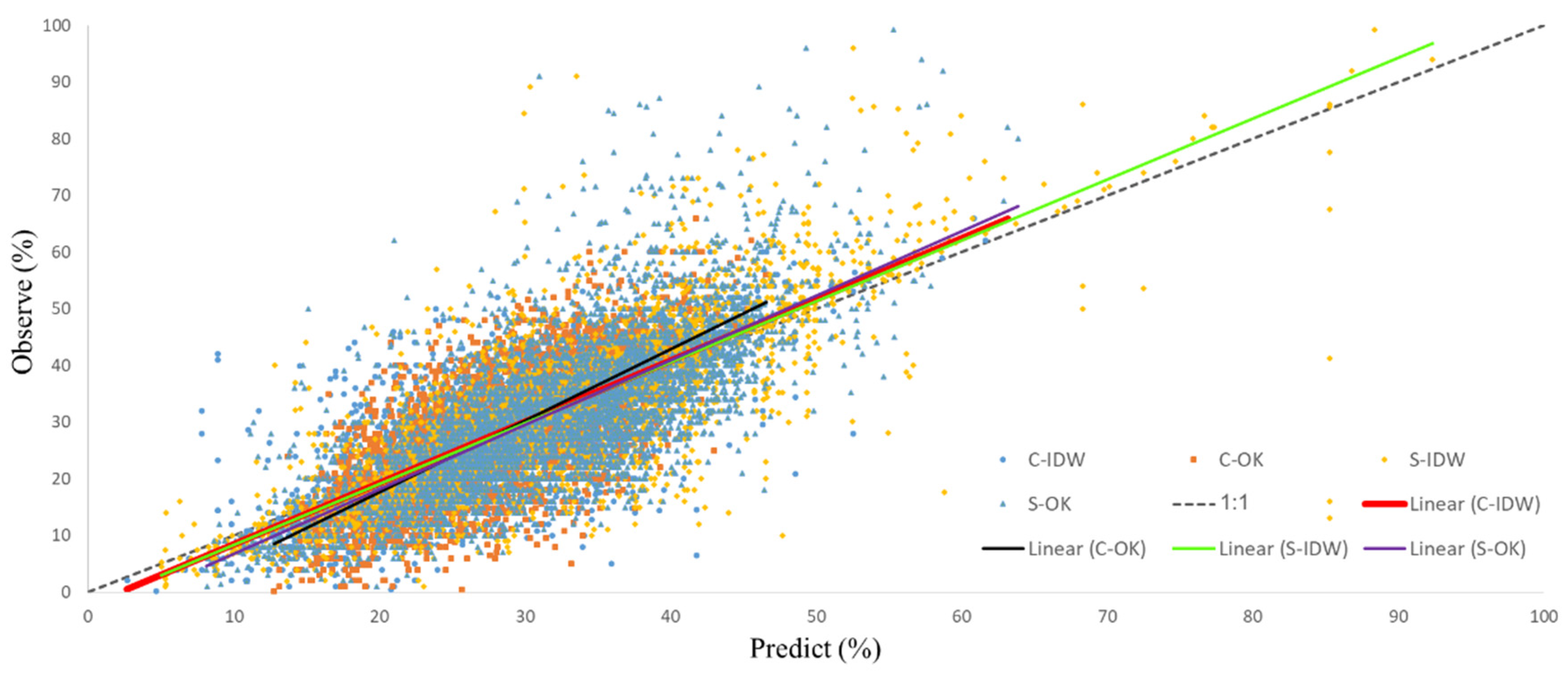
2.8.1. Interpolated Data Evaluation

The validation set provides an unbiased evaluation of the most probable model to avoid overfitting. Four common indices, namely coefficient of determination (R²), mean error (ME) and normalized root of mean squared error (NRMSE) were used for assessing the accuracy of interpolating STFs including sand, silt and clay particles. The MBE is an estimate of the average bias in the interpolation method, and the closer to 0, the lower the bias. Its positive values represent overestimation and its negative values underestimation. NRMSE is a percentage that represents the relative difference of the observed and estimated values. According to [75], NRMSE values of up to 10, 10–20, 20–30 and >30% represent excellent, good, relatively good and poor models, respectively. RMSE represents the predicted model accuracy, while MBE also suggests model performance but with less sensitivity to outliers compared to RMSE.

2.8.2. ANN-Predicted Soil Texture Class Evaluation

The KIA and P_a were used for evaluating the accuracy of the soil texture classification estimation maps. In addition, the identity line (the 1:1 line) was employed to fit the predicted values to the observed values of the variables. The KIA, P_a, MBE, and NRMSE equations are represented as Equations (2)–(5):

$$KIA=\frac{\left(P_0-P_e\right)}{1-P_e}$$

(2)

$$Pa=\frac{{{\displaystyle \sum }}_{j=1}^m\left(C_{\left(sj\right)}^{^}=C_{\left(sj\right)}\right)}{m}$$

(3)

$$MBE=\frac{{\displaystyle \sum }\left(P_i-O_i\right)}{n}$$

(4)

$$NRMSE=\sqrt{\frac{{{\displaystyle \sum }}_{i=1}^n{\left(O_i-P_i\right)}^2}{n}}\times \frac{100}{\overline{O}}$$

(5)

O_i is the observed value, P_i refers to the estimated value, n is the number of observations. KIA is the kappa coefficient, P₀ is the overall accuracy from the confusion matrix, and P_e denotes the hypothetical probability of chance agreement. The KIA is a statistical agreement indicator that calculates the probability of presence or absence of a class estimated by the model. It varies from 0 to 1. KIA values greater than 0.8, 0.8–0.6, 0.6–0.4, 0.4–0.2 and smaller than 0.2 indicate very good, good (strong), moderate, fair and poor agreement, respectively [76]. $C_{\left(sj\right)}^{^}$C is the estimated class at the Sj validation location and $C_{\left(sj\right) }$ the observed class at the Sj location. P_a varies from 0 to 100% and the higher value indicates the closeness between predicted and observed values [31].

2.9. Spatial Predictions

There are two main schemes of classification—pixel-based and object-based approaches—in thematic mapping according to [77]. In a pixel-based approach, image classifications are mostly performed pixel by pixel to produce soil texture classes. The advantages of this classifier correspond to both its capability in using data from different scales and its independence of prior assumptions [78].

In this case, to represent a continuous STCs map, the produced ANN related covariates to soil texture classes at each point. Consequently, the outputs of the most accurate ANN at the unvisited sites were first extracted. Then, the point-source dataset was converted to a pixel-based set after using conversion tools in ArcGIS 10.4, in which each pixel was only assigned to one soil texture class. There are various studies confirming that pixel-based classification is an authentic method for digital soil mapping [38,48,79,80,81,82,83,84].

3. Results and Discussion

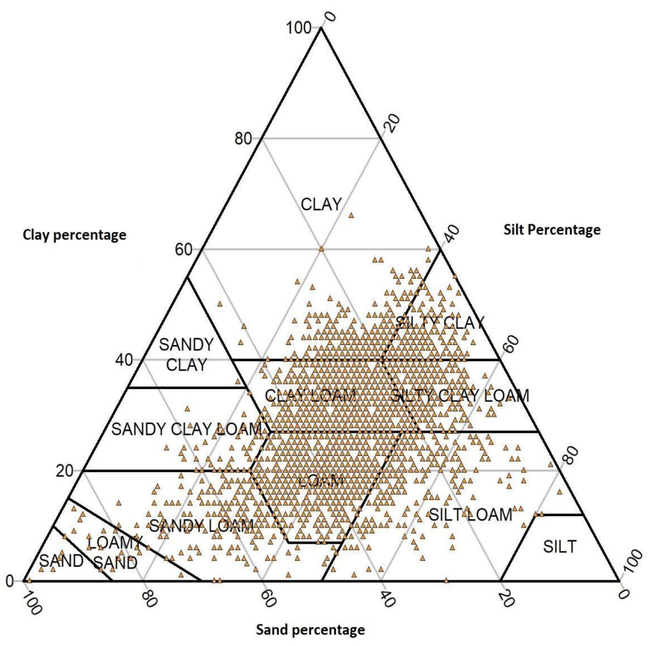
3.1. Soil Dataset Descriptive Statistics

The classical analysis of descriptive statistics related to the topsoil sand, clay and silt particles of the legacy soil dataset of Guilan Province are represented in

Table 3. Statistical summary of STFs of the total dataset for Guilan province (n = 4493).

Particle	Min	Max	AM	GM	Mode	Median	St. Dev	Skewness	Kurtosis	% C.V
Clay (%)	1	66	39.4	29.3	40	29.7	10.6	−0.408 *	−0.408 *	27
Sand (%)	1	99	31.5	30.8	24	30.4	13.4	−1.197 *	0.709 *	43
Silt (%)	1	81	39.8	39.8	42	39.6	9.14	−1.493 *	0.158 *	23

AM: arithmetic mean; GM: geometric mean; St. Dev: standard deviation; CV: coefficient of variation (%); * significance at 5% level.

. The silt fraction presented an average of 39.8%, whereas the clay and sand particles presented 29.3 and 30.8%, respectively. Soil texture fractions have a central tendency for the reason that the values of means are generally greater than the median [85]. Therefore, particular care should be taken to balance the variance in the transformation process [86].

The coefficient of variation (C.V %) was the highest for sand particles (43%) since it varies in a wide range from 1 to 99%. These results are in agreement with those reported by [87] in Mazandaran, a neighboring province. In contrast, clay particles had the lowest variation with 27%, while the variability of silt particles was moderate.

The median, mean and mode values were similar, and skewness and kurtosis were significant at the 5% level, which implies a normal frequency distribution (Table 3). The high coefficient of variation values for the sand particle indicate that this variable has a high level of nonuniform distribution. This may be the consequence of three simultaneous phenomena, namely marine sediments, mountain debris and riparian alluvial deposits, that usually have a bigger effect on the transport of large particles such as sand. Moreover, the accumulation of finer particles in low lands could be attributed to selective particle removal via soil erosion [88]. Despite the normal frequency, the clay particle has a platy kurtic distribution as indicated by the negative kurtosis, which may indicate the overlap of two populations with different means.

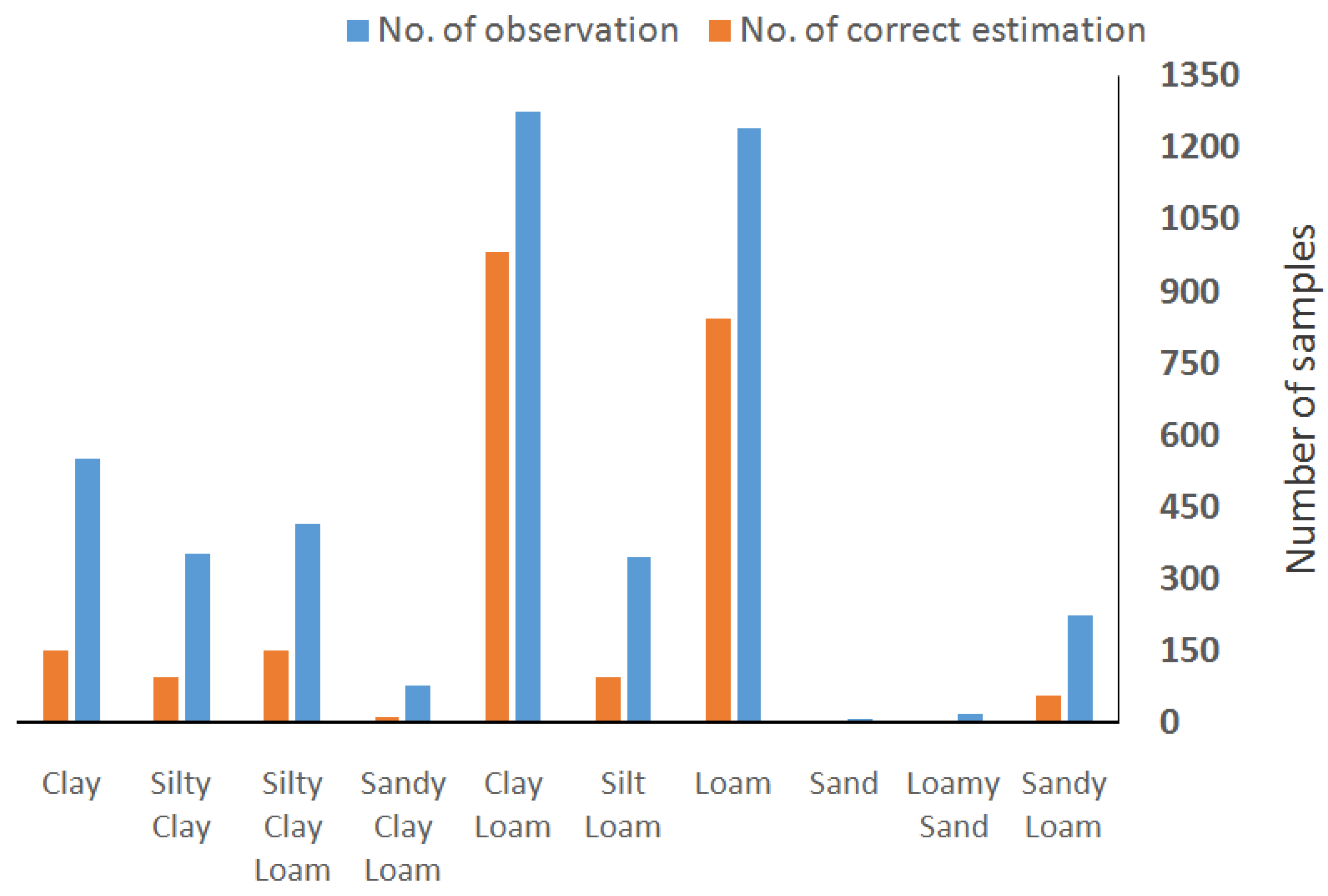
3.2. Soil Texture Class Evaluation

From the 4493 observations, soil textural classes (According to the USDA) were of clay (549 samples), silty clay (352 samples), silty clay loam (414 samples), sandy clay loam (75 samples), clay loam (1274 samples), silt loam (344 samples), loam (1239 samples), sand (6 samples), loamy sand (17 samples), sandy clay (1 sample) and sandy loam (222 samples), as shown in Figure 3. Half of the observational soil texture classes were typically classified as clay loam and loam, given that the silt particle had the maximum arithmetic and geometric mean (Table 3), in which it ranged from 15 to 53%.

3.3. STF Spatial Structure

Geostatistical analysis first required, evaluating the variables in terms of outliers, normality, and isotropy. According to the Norfolk test, 172 samples were considered outliers and omitted from the dataset. The silt and clay particles with a relatively nonnormal distribution were normalized via logarithmic transformations. Detailed results of the spatial structure evaluation of the variables using the components of the best-fitted semi-variogram model are presented in

Table 4. The best-fitted semi-variogram results on sand silt and clay soil particles.

STFs	Model	(C0)	(C0 + C)	A0 (m)	C0/(C0 + C) (%)	R2	RSS
Clay	Expo	60	110	4000	0.54	0.91	86
Sand	Expo	0/13	0/24	6000	0.54	0.94	0.001
Silt	Expo	62	89	8000	0.7	0.93	16.8

C₀: nugget effect; C₀ + C: sill; A₀: range; C₀/(C₀ + C): spatial dependence ratio.

. Obviously, the STFs were fitted using exponential models, where C₀ is the nugget effect, C₀ + C is sill and A₀ is range according to [66].

The semi-variogram model with the lowest RSS and highest R² was the best-fitted and allowed for the mapping of each STF. According to the spatial dependence (nugget to sill), sand and clay particles had moderate structure, whereas sill of silt particles found was 0.7%—which often means that the spatial dependency is relatively high—in the present sampling. Zhang et al. [34] investigated the spatial structure of soil texture fractions and showed that a ratio of C₀/(C₀ + C) > 50% was related to their nonuniform susceptibility to random components. Under such conditions, the interpolation techniques, which are a subset of spatial statistics based on spatial correlation of variables, are less efficient. The spatial distribution of mineral soil particles in the fields of Guilan Province appears to be affected by the sediment load from the Sepidrud River, mountain debris from the Alborz range and coastal sediments in addition to soil parent materials. Moreover, the variables of soil mineral particles showed regional non-isotropy (results not presented). Therefore, the anisotropic orientation was considered in the search radius for the OK interpolation method. In addition, all particles of the best-fitted model had a rather low nugget effect, meaning that the studied soils are homogeneous. This can be attributed to puddling practices and similar rice cultivation over the study area. Higher effective range produced a large patch over the continuous PSF map in silt and sand particles in particular (Figure 4a).

The accuracy assessment of the clay and sand particles using OK and IDW methods and deviation from the identity line (Figure 5) shows their goodness-of-fit (silt particle results not presented). A comparison of the predicted and observed values for the two interpolation methods of sand and clay particles against the identity line showed that IDW had a near-zero intercept, a slope closer to 1, and a higher coefficient of determination (Figure 5). The IDW method performed more accurately for clay and sand particles based upon lower NRMSE, ME and R² statistics of 0.22; 0.02 and 0.64; and 0.25, 0.03 and 0.67; respectively (

Table 5. Statistics validation of sand and clay particles interpolation.

Variable	Interpolation Method	R2	RMSE	NRMSE	d	ME	Equation
Clay	OK	0.54	7.3	0.25	0.8	0.006	y = 0.4365x + 16.366
	IDW	0.64	6.4	0.22	0.87	0.023	y = 0.5962x + 11.762
Sand	OK	0.52	9.3	0.29	0.8	0.29	y = 0.4565x + 17.429
	IDW	0.67	7.9	0.25	0.87	0.03	y = 0.6039x + 12.518

R²: coefficient of determination; RMSE: root mean square error; NRMSE: normalized root mean square error, d: index of agreement; ME: mean error; y: observe; x: predict.

).

Researchers have reported improvements in STFs predicting problems using machine-learning techniques in general. For instance, a key improvement was reported by [40] for clay particle prediction even with an RMSE of less than 1. In the present study, clay particle results achieved better ME and moderate RMSE as compared to other studies (

Table 6. Overview of selected research findings on STFs large-scale estimations.

Reference	No of Samples	Depth (cm)	Method	Particles
				Sand						Silt		Clay
				Fine Sand		Coarse Sand		Sand
				ME	RMSE	ME	RMSE	ME	RMSE	ME	RMSE	ME	RMSE
Zhao et al., 2009 [42]	442	NA	ANN LM	NA	NA	NA	NA	8.11	16.6	NA	NA	1.18	7.9
			ANN RP	NA	NA	NA	NA	1.12	14.9	NA	NA	2.07	8.5
Greve et al., 2012 [36]	45,224	0–30	RT	7.54	11.31	8.64	12.46	NA	NA	2.51	12.41	2.27	11.41
Wang et al., 2015 [25]	62	Topsoil	LRM	NA	NA	NA	NA	8.72	10.69	NA	NA	3.44	4.57
Song et al., 2016 [39]	119	0–120	ANN RF	NA	NA	NA	NA	NA	12.5	NA	NA	NA	3
Mehrabi et al., 2019 [38]	115	0–5	RT	NA	NA	NA	NA	0.09	6.98	0.21	4.64	0.04	5.07
			ANN	NA	NA	NA	NA	0.06	4.07	0.1	2.75	0.02	2.02
			ANFIS	NA	NA	NA	NA	0.06	4	0.09	2.68	0.02	2
Wang et al., 2020 [40]	640	0–20	ALR-BRT	NA	NA	NA	NA	0.57	15.99	−2.23	15.1	NA	1.75
			ALR-RF	NA	NA	NA	NA	0.38	15.7	−1.78	14.53	NA	1.4
			ALR-RK	NA	NA	NA	NA	−2.34	17.92	0.86	17.05	NA	1.49
			ILR-BRT	NA	NA	NA	NA	0.84	15.56	−2.44	14.71	NA	1.6
			ILR-RF	NA	NA	NA	NA	0.51	15.35	−1.89	14.2	NA	1.38
			ILR-RK	NA	NA	NA	NA	−2.66	16.91	1.77	16.6	NA	0.89
Khanbabakhani et al., 2020	105	0–15	ANN	NA	NA	NA	NA	NA	4	NA	4	NA	4
Zhou et al., 2022 [1,37]	943	0–20	SVM and SHAP	NA	NA	NA	NA	NA	NA	NA	NA	NA	NA

LM: Levenberg-Marquardt algorithm; RP: resilient algorithm; LRM: linear regression models; RT: regression-tree; ANN: artificial neural network; RF: random forest; ANFIS: neuro-fuzzy technique; ALR: additive log-ratio; BRT: boosted regression tree; RK: regression kriging; ILR: isometric log-ratio; NA: not available (not reported or used).

). There was no improvement in the prediction of sand particles in extensive studies, which reflects that the problems of this soil particle still remain. However, the results showed better estimates of sand particles than advanced methods such as machine learning. The authors of this study believe that non-isotropic spatial distribution of sand particles corresponds to the frequent disposal mainly caused by periodic variation in sea level, particularly in coastal areas. Toposequence is another driven factor that forms different physiographic units [89]. Coarse residuals are transported via mountains (colluvium) and alluvial plains to lowlands where the distance between mountain and sea is minimum. This mostly happened in eastern and western parts of the study region (Figure 4c).

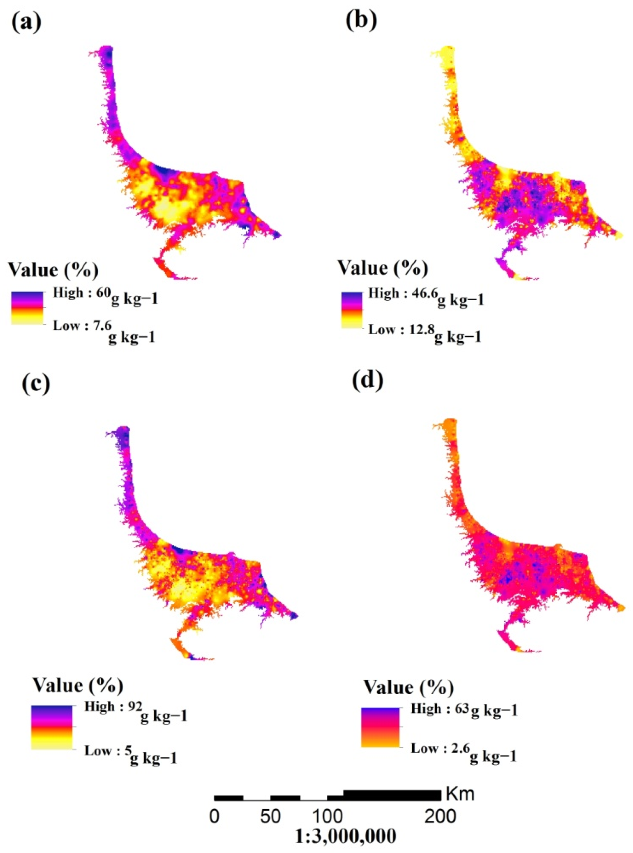
3.4. Soil Texture Fraction Mapping

The OK estimation for clay the fraction ranged between 12 and 46% (Figure 4b), while the IDW values varied from 2 to 63% (Figure 4d), which is closer to the observed values (1–66%). The values for the sand particles were between 7 and 60% using OK (Figure 4a) and 5 and 92% (Figure 4c) with IDW. However, the observed values of sand particles in Guilan Province ranged from 1 to 99% [29]. The regions located in the central part of the province had higher clay and lower sand particle content, which originated from the Sepidrud River’s sediment load. The areas in the eastern and western parts of the area, where there is a short distance between the mountainous and the Caspian Sea, contained higher a sand percentage in both (Figure 4). Alteration, suitable aeration and occurrence of ferrolysis lead to lower clay particle content in plateaued lands [89].

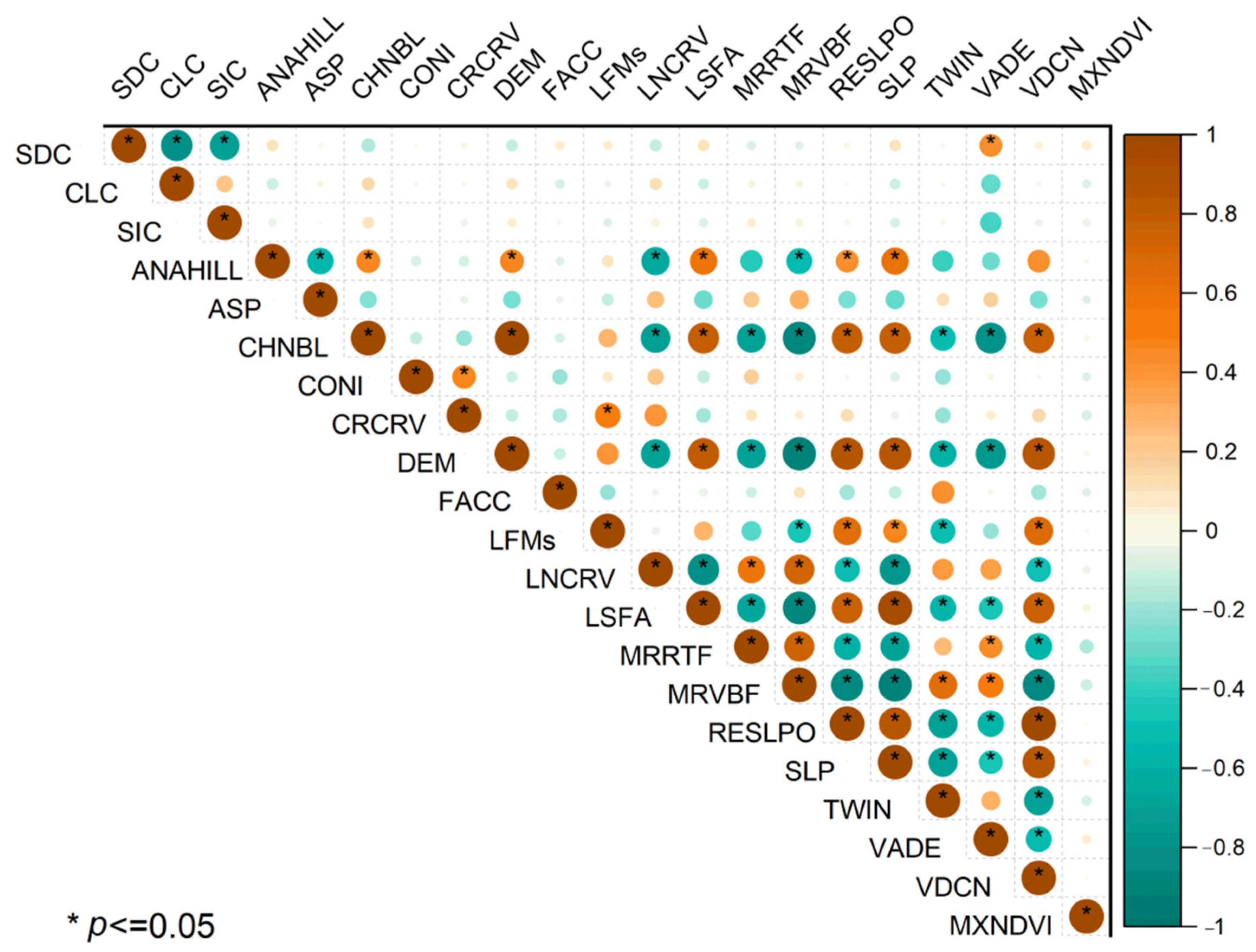
3.5. Important Covariates

The linear correlation matrix analysis of all environmental and soil-related covariates showed that 130 and 9 out of 210 paired comparisons were significant at 5% and 1% levels of confidence, respectively (Figure 6). This supports the reduction and also the selection of the most important covariates to avoid robust parallel correlation and covariance metrics. In addition, there were several negative correlations between covariates where the greatest rose between the channel network base level and DEM.

As can be seen, some of the covariates had more influence on the soil texture class predictions according to the removal method as a multiplelinear regression in the context of sensitivity analysis (

Table 7. Sensitivity analysis of related sets of covariates results.

Covariates	B	Std. Error	St. B	P.co	T	p-Value
CLC	0.051	0.005	0.156	0.162	10.270	0.000
SIC	−0.007	0.006	−0.019	−0.031	−1.273	0.038
ANAHILL	−0.383	0.531	−0.012	−0.006	−0.721	0.471
ASP	0.009	0.026	0.006	0.007	0.371	0.662
CHNBL	0.014	0.014	0.160	0.083	1.009	0.000
CONI	0.002	0.003	0.007	0.005	0.483	0.629
CRCRV	229.050	288.751	0.014	0.027	0.793	0.428
DEM	−0.008	0.014	−0.111	0.080	−0.588	0.000
FACC	2.820 × 10−10	0.000	0.003	−0.002	0.209	0.835
LFMs	−0.059	0.157	−0.007	0.032	−0.375	0.034
LNCRV	287.705	247.781	0.022	0.004	1.161	0.246
LSFA	−0.157	0.099	−0.056	0.032	−1.586	0.031
MRRTF	−0.145	0.034	−0.072	−0.0081	−4.308	0.000
MRVBF	0.061	0.051	0.028	−0.053	1.196	0.232
RESLPO	−247.250	67.044	−0.563	0.042	−3.688	0.000
SLP	5.694	2.881	0.086	0.053	1.976	0.000
TWIN	0.004	0.022	0.003	−0.019	0.161	0.202
VADE	0.000	0.001	−0.010	−0.053	−0.495	0.000
VDCN	0.132	0.036	0.591	0.047	3.688	0.000
MXNDVI	−0.313	0.432	−0.011	−0.012	−0.725	0.468

SDC: sand particle content; CLC: clay particle content; SIC: silt particle content; ANAHILL: analytical hill-shading; ASP: aspect; CHNBL: channel network base level; CONI: convergence index; CRCRV: cross-sectional curvature; DEM: digital elevation model; FACC: flow accumulation; LFMs: landforms; LNCRV: longitudinal curvature; LSFA: LS factor; MRRTF: multiresolution index of the ridgetop’s flatness; MRVBF: multiresolution index of the valley bottom’s flatness; RESLPO: relative slope position; SLP: slope; TWIN: topographic wetness index; VADE: valley depth; VDCN: vertical distance to channel network; MXNDVI: max NDVI (normalized difference vegetation index); B: unstandardized beta coefficient; Std. Error: standard error; St. B: standardized beta coefficient; P.co: partial correlation.

). It should be noted that these covariates selected by statistics are only beneficial for the modelling of soil texture classes and they are useless to explicit soil process and SCORPAN components. The most effective covariates were clay particles, DEM, channel network base level, relative slope position, slope, valley depth, vertical distance to channel network, MRRTF and cross-sectional curvature, respectively, in order of P-value and partial correlation metric. Surprisingly, time-series NDVI (normalized difference vegetation index) as plant indices derived from reflection-based satellite data were excluded, which is exactly the opposite of results reported by [1], which indicated that elevation, stratum and red-edge factors are critical variables for the prediction of soil texture classes. This is related to the site-specific-dependent prediction of soil texture class modelling. For instance, authors of [28] identified curvature parameters such as the shape of the slope as the most important predictive variables in a flood plain, while the stratum (legacy soil maps) and red-edge electromagnetic spectrum in addition to elevation were discovered as critical variables topredicting soil texture classes in multi-crop farming and the humid, subtropical monsoon climate of southwestern China [1]. In addition, authors of [28] reported elevation, slope, MRVBF, NDVI and B3 as critical variables. This can be due to the diversity in elevation (from 315 to 500 m above sea levels) and land use types that are cultivated in the regions.

These results were in line with those reported by [5,37,41,42], which where mostly located in areas with dense vegetation cover. They realized that terrain attributes have a great influence on the prediction of soil texture class. Notably, surface sand particle content was without any influence on the estimation of soil texture class against clay particle content of surface soil.

3.6. Soil Texture Class Prediction Performance

Pixel-based classification combined with ANN was used to estimate the soils’ textural classes in the unvisited pixels in which the texture class was unclear. Since IDW is superior in estimating sand, silt and clay particle content at unvisited points (Table 5), its continuous mapoutput was used as the network’s input variable. The ANN was trained very well using accuracy evaluation statistics. The training (2995 samples) and testing (1498 samples) achieved R² 0.98, RMSE 0.07 and 0.94, 0.08, respectively. This demonstrated its capability in determining each pixel of the regions without any soil texture class data. Results showed remarkable outputs for the predictive model in terms of the coefficient of determination and RMSE for the calibration dataset.

The aim of the accuracy assessment was to numerically assess how effectively the pixels (samples) were observed into the corresponding soil texture classes (Table 5). The confusion matrix displays the soil texture classes in the reference dataset as columns and the same information as in the output dataset. The individual cells within the table indicate the number of samples with a given combination of reference data and output data. Looking down the first row (A) (

Table 8. Confusion matrix of actual and predicted soil texture classes.

Class	C	S	LS	SL	SIC	SICL	SC	SCL	CL	SIL	L	Observation
C	147	-	0	0	19	24	-	0	334	0	25	549
S	0	-	3	0	0	0	-	0	1	0	2	6
LS	0	-	1	7	0	0	-	1	3	0	5	17
SL	0	-	2	53	0	0	-	3	26	1	137	222
SIC	20	-	0	0	92	75	-	0	157	2	6	352
SICL	2	-	0	0	12	146	-	0	201	13	40	414
SC	0	-	0	0	0	0	-	0	1	0	0	1
SCL	0	-	0	2	0	0	-	9	24	0	40	75
CL	20	-	0	5	6	39	-	5	979	2	218	1274
SIL	1	-	0	2	0	18	-	0	59	93	171	344
L	3	-	1	12	4	11	-	1	345	22	840	1239
Total	193	-	7	81	133	313	-	19	2130	133	1484	4493

C: clay; S: sand; LS: loamy sand; SL: sandy loam; SIC: silty clay; SICL: silty clay loam; SC: sandy clay; SCL: sandy clay loam; CL: clay loam; SIL: siltyloam; L: loam.

), out of 549 samples for clay soil texture class, 147 were classified correctly, and from the rest, 19 were indicated as silty clay, and 24 and 25 as silty clay loam and loam soil texture classes, respectively. However, the ANN could not achieve reasonable accuracy for more than 60% of soil texture classes within a class. The results from the error matrix show that in all textural classes, there were some samples representing other ones. It should be noted that the imbalanced distribution of STCs may have affected the results [90]. Nevertheless, out of 4493 samples, 2360 were predicted correctly. This finding was inconsistent with those reported by Kaya et al. [91] who used an RF algorithm to predict soil texture classes in northwestern Türkiye.

The evaluation of results according to the statistics showed that the ANN method achieved a reasonable pixel classification accuracy percentage (Pa) of 55% (

Table 9. Accuracy assessment results of the studied area’s soil texture class prediction map.

Soil Texture Class	Reference Totals	Classified Totals	Number Correct	PA	UA
Clay	193	549	147	76%	27%
Sand	0	6	0	0%	0%
Loamy sand	7	17	1	14%	6%
Sandy loam	81	222	53	65%	24%
Silty clay	133	352	92	69%	26%
Silty clay loam	313	414	146	46%	35%
Sandy clay	0	1	0	0%	0%
Sandy clay loam	19	75	9	47%	12%
Clay loam	2130	1274	979	46%	77%
Silt loam	133	344	93	70%	27%
Loam	1484	1239	840	56%	68%
Total	4493	4493	2360	55%	33.5%

PA: producer accuracy; UA: user accuracy. Overall accuracy = 52.53%; kappa = 0.38.

). In addition, the value of the kappa coefficient (0.38) using the ANN classification showed strong agreement between predicted and observed soil texture classes. The model performance for each class was examined individually and a noticeable improvement arose for 10 out of 12 soil texture classes. This finding was also in harmony with previous studies, such as [5,24], who could not correctly predict silt loam and clay loam classes using multiple stepwise regression and cokriging, and old soil texture classes of loose sand, light sand, medium clay and heavy clay using ANN, respectively, both in China. Uniquely, authors of [30] effectively predicted six soil texture classes of clay, sand, sandy loam, sandy clay loam, sandy clay and sandy loam with 120 surface soil samples (0–30 cm) in an arid region of central Iran. We believe that the analogous sampling depth with choice of method have a considerable effect on the success of estimates just as others [30,41] have examined surface soil samples against different approaches. Additionally, the variety of soil texture classes may affect the results. For example, Kaya et al. [91] employed five out of 12 soil texture classes that obtained an overall accuracy of 0.63 and a kappa index value of 0.14.

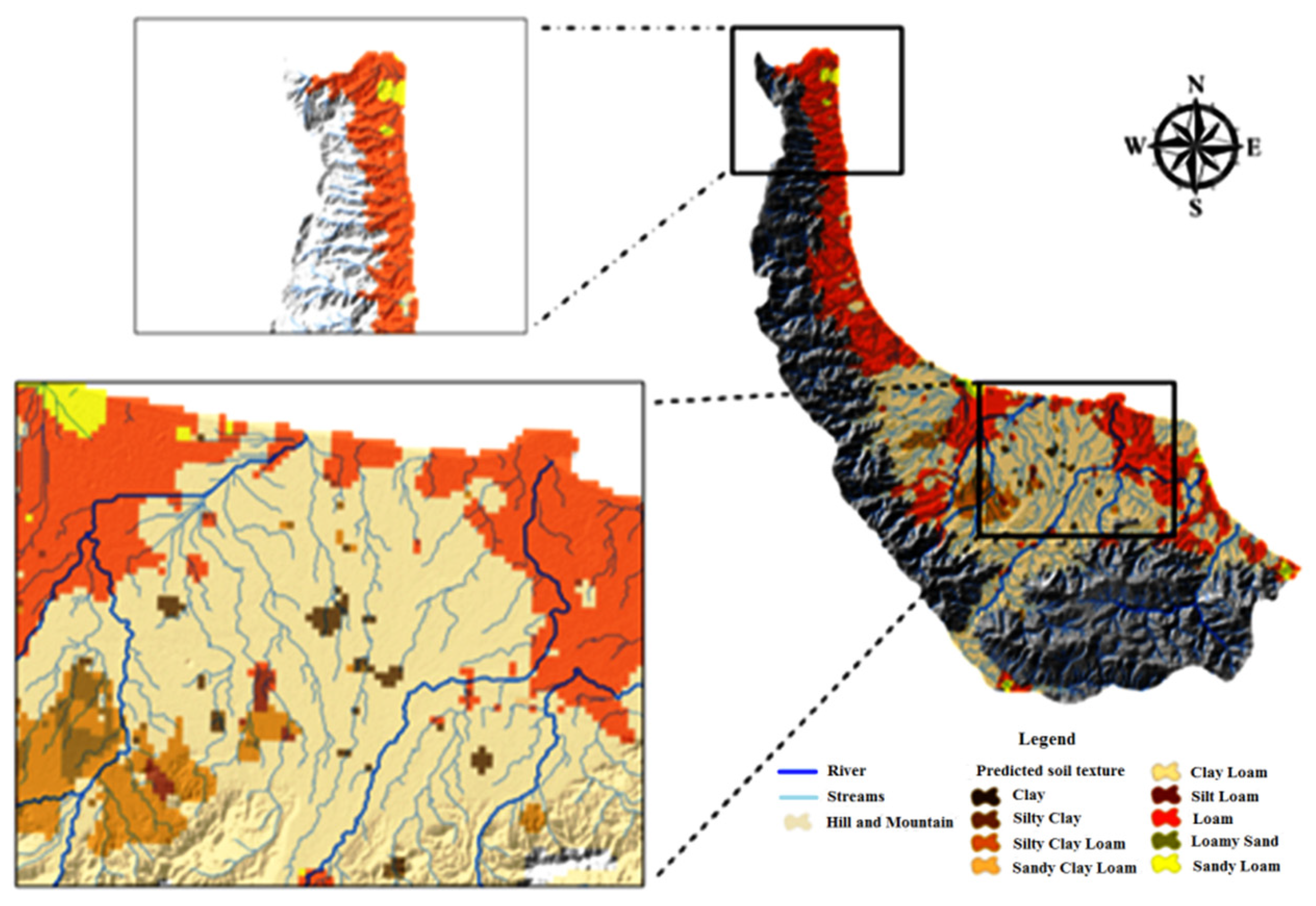
3.7. Predicted Soil Texture Class Map

Ten main USDA soil texture classes were detected, namely sandy loam, sand, loamy sand, loam, silty loam, clay loam, sandy clay loam, silty clay loam, silty clay and clay. The PBC predicted the loam and loam clay textural classes appropriately. These two classes had a higher number of samples compared to the other ones. Moreover, estimation accuracy was lower in fine-textured classes (sand, loamy sand, sandy loam, sandy clay loam) in which the sand particle was the predominant component in all discussed classes. This can be attributed to the low number of fine-textured class samples that had a lower share in the training dataset as well as a poorer relationship between the covariates and sand particle contents. This is in disagreement with findings by authors of [92,93,94], who worked in areas with higher sand particle content compared with silt and clay particle content. They had a diverse range of samples (50–1958 soil profiles) and a low variety of soil texture classes, which was in strong contrast to our research. Furthermore, it is noteworthy, however, that the clayey soil texture classes, despite having a higher number of samples, had a lower accuracy than the medium-textured classes such as loamy clay silt, clay silt, and loamy silt (Figure 7).

The most probable map produced by using the PBC approach using resampled data is represented in Figure 8. PBC was successful in estimating coarse-textured classes, especially in the central region where the soils contained less clay and more sand particles. The loam, loamy sand and sandy loam classes were mapped in the northern regions, which are almost coastal. The clayey loam class dominated in the center, and other classes were scarcely distributed in the study area. With respect to the predicted clay particle map (Figure 4d), there was higher clay content in the central than the southern region of the province, which matched with the river delta and flooding are as where the fine-texture particles are dominantly sedimented [87]. Moreover, clayey loam and silty clay loam heavy soil texture classes mostly happened in areas where four main rivers and their main stream meanders change over time due to fluctuation in water flow [95]. The samples with clay particle contents accounted for over 40% and mainly occurred at lower elevation. In comparison with clayey soil texture classes, the sand particle content was higher in the coastline edge of Caspian Sea, especially in the northwest, where the lands are mostly degraded, and parent materials are prone to erosion. Morphological characteristics and, accordingly, soil physical characteristics of paddy fields are highly influenced by artificial flooding and periodic wet (higher vermiculite/smectite ratio) and dry (lower vermiculite/smectite ratio) conditions [95].

Despite the fact that verification statistics (Table 8) confirm that PBC had reasonable accuracy, authors of [96] stated that ignoring the information on neighboring pixels may be beneficial to correctly identifying the target pixel’s class. This is one of the limitations of pixel-based classification. Indeed, it was expected that when the quantitative variables of sand, silt and clay particles were transformed into the qualitative variables of the soils’ textural class, the spatial similarity of the data as well as the effectiveness of the IDW interpolation method would increase. However, these expectations were not met in this research.

The IDW interpolation method is based on the hypothesis that the degrees of correlation and similarity between adjacent samples correspond to the distance between them. It seems that the abrupt soil texture class changes in the central part of the study area compared to its eastern and western parts, and the lack of the required number of samples, were among the most probable reasons for the increased uncertainty in estimating soil textural classes using this method, which was not feasible due to the high costs of sampling and lab measurement. The produced map can potentially be utilized as a base map for the agro-ecological modelling of future studies. Paddy rice fields should be developed in the clayey soil texture classes’ central parts to restrict water from penetrating the soil profile, while irrigation mismanagement in sandy soil texture class regions may lead to water loss and fertilizer leaching.

4. Conclusions

The proposed hybrid architecture was able to accurately predict and map various soil texture classes. Among considered covariates, soil texture fractions, specifically clay particles, made a significant contribution to modelling soil textural classes. This means without such an approach, we may fail to reach an accurate STC prediction using DSM.

IDW outperformed OK and produced better results for all STFs. Once combining STF data with multi environmental covariates (mainly terrain) the hybridized approach resulted in better performance across all metrics. ANN was able to find the nonlinear relationships between variables, which improves uncertainties. This advantage was more pronounced in the loam and loamy clay textural classes. We observed that the punctual value was better-estimated than the soil class value.

We highlighted the importance of contextual information in accordance with the geographical environment for soil texture studies. Since the vegetation cover of the area is almost evergreen, even the use of RS-based datasets adds more complexity to the modelling procedure. The ANN pixel-based classification method using hybridization of soil particles and terrain attributes proved beneficial in estimating such qualitative data, specifically in single crop-covered areas.

The high-resolution STFs and pixel-based USDA soil textural class maps prepared in this study can be practiced for integrated soil and water management to facilitate sustainable agricultural production even at regional scale. Access to legacy soil databases and producing large geographical maps of soil stable properties, i.e., soil texture classes is vital for sustainable land management and land use planning. They can also reduce laboratory test expenses and provide serviceable information to decisionmakers at the farm level with respect to irrigation and drainage management, and agricultural mechanization. The use of the proposed architecture for predicting soil texture class with a balanced number of observations using other models and in areas with multiple crop types is highly recommended for further research.

References

1. Zhou, Y.; Wu, W.; Wang, H.; Zhang, X.; Yang, C.; Liu, H. Identification of Soil Texture Classes Under Vegetation Cover Based on Sentinel-2 Data with SVM and SHAP Techniques. IEEE J. Sel. Top. Appl. Earth Obs. Remote Sens. 2022, 15, 3758–3770. [Google Scholar] [CrossRef]
2. Gozdowski, D.; Stępień, M.; Samborski, S.; Dobers, E.S.; Szatyłowicz, J.; Chormański, J. Determination of the Most Relevant Soil Properties for the Delineation of Management Zones in Production Fields. Commun. Soil Sci. Plant Anal. 2014, 45, 2289–2304. [Google Scholar] [CrossRef]
3. Bakker, A. Soil Texture Mapping on a Regional Scale with Remote Sensing Data. Ph.D. Thesis, Wageningen University, Wageningen, The Netherlands, 2012. [Google Scholar]
4. Bouma, J.; Stoorvogel, J.; Van Alphen, B.; Booltink, H. Pedology, Precision Agriculture, and the Changing Paradigm of Agricultural Research. Soil Sci. Soc. Am. J. 1999, 63, 1763–1768. [Google Scholar] [CrossRef] [Green Version]
5. Ding, X.; Zhao, Z.; Yang, Q.; Chen, L.; Tian, Q.; Li, X.; Meng, F.-R. Model Prediction of Depth-Specific Soil Texture Distributions with Artificial Neural Network: A Case Study in Yunfu, a Typical Area of Udults Zone, South China. Comput. Electron. Agric. 2020, 169, 105217. [Google Scholar] [CrossRef]
6. Koseva, I.S.; Watmough, S.A.; Aherne, J. Estimating Base Cation Weathering Rates in Canadian Forest Soils Using a Simple Texture-Based Model. Biogeochemistry 2010, 101, 183–196. [Google Scholar] [CrossRef]
7. Ghiri, M.N.; Abtahi, A. Factors Affecting Potassium Fixation in Calcareous Soils of Southern Iran. Arch. Agron. Soil Sci. 2012, 58, 335–352. [Google Scholar] [CrossRef]
8. Goli-Kalanpa, E.; Roozitalab, M.; Malakouti, M. Potassium Availability as Related to Clay Mineralogy and Rates of Potassium Application. Commun. Soil Sci. Plant Anal. 2008, 39, 2721–2733. [Google Scholar] [CrossRef]
9. Vaughan, E.; Matos, M.; Ríos, S.; Santiago, C.; Marín-Spiotta, E. Clay and Climate Are Poor Predictors of Regional-Scale Soil Carbon Storage in the US Caribbean. Geoderma 2019, 354, 113841. [Google Scholar] [CrossRef]
10. Xu, H.; Liu, K.; Zhang, W.; Rui, Y.; Zhang, J.; Wu, L.; Colinet, G.; Huang, Q.; Chen, X.; Xu, M. Long-Term Fertilization and Intensive Cropping Enhance Carbon and Nitrogen Accumulated in Soil Clay-Sized Particles of Red Soil in South China. J Soils Sediments 2020, 20, 1824–1833. [Google Scholar] [CrossRef]
11. Bockheim, J.; Hartemink, A. Distribution and Classification of Soils with Clay-Enriched Horizons in the USA. Geoderma 2013, 209, 153–160. [Google Scholar] [CrossRef]
12. Reichardt, K.; Timm, L.C. Solo, Planta e Atmosfera: Conceitos, Processos e Aplicações; Manole: Barueri, Brazil, 2004. [Google Scholar]
13. Dupuis, E.M.; Whalen, J.K. Soil Properties Related to the Spatial Pattern of Microbial Biomass and Respiration in Agroecosystems. Can. J. Soil Sci. 2007, 87, 479–484. [Google Scholar] [CrossRef]
14. Taghizadeh-Mehrjardi, R.; Mahdianpari, M.; Mohammadimanesh, F.; Behrens, T.; Toomanian, N.; Scholten, T.; Schmidt, K. Multi-Task Convolutional Neural Networks Outperformed Random Forest for Mapping Soil Particle Size Fractions in Central Iran. Geoderma 2020, 376, 114552. [Google Scholar] [CrossRef]
15. Behrens, T.; Zhu, A.-X.; Schmidt, K.; Scholten, T. Multi-Scale Digital Terrain Analysis and Feature Selection for Digital Soil Mapping. Geoderma 2010, 155, 175–185. [Google Scholar] [CrossRef]
16. Klein, V.A.; Baseggio, M.; Madalosso, T.; Marcolin, C.D. Soil Texture and the Estimation by Dewpoint Potential Meter of Water Retention at Wilting Point/Textura Do Solo e a Estimativa Do Teor de Agua No Ponto de Murcha Permanente Com Psicrometro. Ciência Rural 2010, 40, 1550–1557. [Google Scholar] [CrossRef] [Green Version]
17. Tümsavaş, Z.; Tekin, Y.; Ulusoy, Y.; Mouazen, A.M. Prediction and Mapping of Soil Clay and Sand Contents Using Visible and Near-Infrared Spectroscopy. Biosyst. Eng. 2019, 177, 90–100. [Google Scholar] [CrossRef]
18. Malone, B.P.; McBratney, A.B.; Minasny, B. Spatial Scaling for Digital Soil Mapping. Soil Sci. Soc. Am. J. 2013, 77, 890–902. [Google Scholar] [CrossRef] [Green Version]
19. Paterson, S.; Minasny, B.; McBratney, A. Spatial Variability of Australian Soil Texture: A Multiscale Analysis. Geoderma 2018, 309, 60–74. [Google Scholar] [CrossRef]
20. Mesgaran, M.B.; Madani, K.; Hashemi, H.; Azadi, P. Iran’s Land Suitability for Agriculture. Sci Rep 2017, 7, 7670. [Google Scholar] [CrossRef] [Green Version]
21. Roozitalab, M.H.; Toomanian, N.; Ghasemi Dehkordi, V.R.; Khormali, F. Major Soils, Properties, and Classification. In The Soils of Iran; Springer: Berlin/Heidelberg, Germany, 2018; pp. 93–147. [Google Scholar]
22. Zeraatpisheh, M.; Jafari, A.; Bagheri Bodaghabadi, M.; Ayoubi, S.; Taghizadeh-Mehrjardi, R.; Toomanian, N.; Kerry, R.; Xu, M. Conventional and Digital Soil Mapping in Iran: Past, Present, and Future. Catena 2020, 188, 104424. [Google Scholar] [CrossRef]
23. Ryżak, M.; Bieganowski, A. Methodological Aspects of Determining Soil Particle-size Distribution Using the Laser Diffraction Method. J. Plant Nutr. Soil Sci. 2011, 174, 624–633. [Google Scholar] [CrossRef]
24. Liao, K.; Xu, S.; Wu, J.; Zhu, Q. Spatial Estimation of Surface Soil Texture Using Remote Sensing Data. Soil Sci. Plant Nutr. 2013, 59, 488–500. [Google Scholar] [CrossRef]
25. Wang, D.-C.; Zhang, G.-L.; Zhao, M.-S.; Pan, X.-Z.; Zhao, Y.-G.; Li, D.-C.; Macmillan, B. Retrieval and Mapping of Soil Texture Based on Land Surface Diurnal Temperature Range Data from MODIS. PLoS ONE 2015, 10, e0129977. [Google Scholar] [CrossRef]
26. Goovaerts, P. Geostatistical Tools for Characterizing the Spatial Variability of Microbiological and Physico-Chemical Soil Properties. Biol. Fertil. Soils 1998, 27, 315–334. [Google Scholar] [CrossRef] [Green Version]
27. Kaya, F.; Başayiğit, L. Spatial Prediction and Digital Mapping of Soil Texture Classes in a Floodplain Using Multinomial Logistic Regression. In International Conference on Intelligent and Fuzzy Systems; Springer: Cham, Switzerland, 2021; pp. 463–473. [Google Scholar]
28. Amirian-Chakan, A.; Minasny, B.; Taghizadeh-Mehrjardi, R.; Akbarifazli, R.; Darvishpasand, Z.; Khordehbin, S. Some Practical Aspects of Predicting Texture Data in Digital Soil Mapping. Soil Tillage Res. 2019, 194, 104289. [Google Scholar] [CrossRef]
29. Mallah, S.; Delsouz Khaki, B.; Davatgar, N.; Bazargan, K.; Vahed, H.S.; Rezaee, L.; Shakouri Katigari, M.; Shokri Vahed, H.; Sheikholeslam, H.; Shirinfekr, A. Comparison of Three Geostatistics Methods for Prediction of Soil Texture Classes in Crop and Orchard Lands of Guilan Province. Iran. J. Soil Res. 2019, 33, 213–225. [Google Scholar]
30. Zaeri, K.; Hazbavi, S.; Toomanian, N.; Zadeh, J.T. Creating Surface Soil Texture Map with Indicator Kriging Technique: A Case Study of Central Iran Soils. Int. J. Agric. Crop Sci. (IJACS) 2013, 6, 518–521. [Google Scholar]
31. Hengl, T.; Toomanian, N.; Reuter, H.I.; Malakouti, M.J. Methods to Interpolate Soil Categorical Variables from Profile Observations: Lessons from Iran. Geoderma 2007, 140, 417–427. [Google Scholar] [CrossRef]
32. Ma, Y.; Minasny, B.; Malone, B.P.; Mcbratney, A.B. Pedology and Digital Soil Mapping (DSM). Eur. J. Soil Sci. 2019, 70, 216–235. [Google Scholar] [CrossRef]
33. McBratney, A.B.; Mendonça Santos, M.L.; Minasny, B. On Digital Soil Mapping. Geoderma 2003, 117, 3–52. [Google Scholar] [CrossRef]
34. Zhang, S.; Shen, C.; Chen, X.; Ye, H.; Huang, Y.; Lai, S. Spatial Interpolation of Soil Texture Using Compositional Kriging and Regression Kriging with Consideration of the Characteristics of Compositional Data and Environment Variables. J. Integr. Agric. 2013, 12, 1673–1683. [Google Scholar] [CrossRef] [Green Version]
35. Padarian, J.; Minasny, B.; McBratney, A.B. Machine Learning and Soil Sciences: A Review Aided by Machine Learning Tools. Soil 2020, 6, 35–52. [Google Scholar] [CrossRef] [Green Version]
36. Greve, M.H.; Kheir, R.B.; Greve, M.B.; Bøcher, P.K. Quantifying the Ability of Environmental Parameters to Predict Soil Texture Fractions Using Regression-Tree Model with GIS and LIDAR Data: The Case Study of Denmark. Ecol. Indic. 2012, 18, 1–10. [Google Scholar] [CrossRef]
37. Khanbabakhani, E.; Torkashvand, A.M.; Mahmoodi, M.A. The Possibility of Preparing Soil Texture Class Map by Artificial Neural Networks, Inverse Distance Weighting, and Geostatistical Methods in Gavoshan Dam Basin, Kurdistan Province, Iran. Arab. J. Geosci. 2020, 13, 237. [Google Scholar] [CrossRef]
38. Mehrabi-Gohari, E.; Matinfar, H.R.; Jafari, A. The Spatial Prediction of Soil Texture Fractions in Arid Regions of Iran. Soil Syst. 2019, 3, 65. [Google Scholar] [CrossRef] [Green Version]
39. Song, X.-D.; Liu, F.; Zhang, G.-L.; Li, D.-C.; Zhao, Y.-G. Estimation of Soil Texture at a Regional Scale Using Local Soil-Landscape Models. Soil Sci. 2016, 181, 435–445. [Google Scholar] [CrossRef]
40. Wang, Z.; Shi, W.; Zhou, W.; Li, X.; Yue, T. Comparison of Additive and Isometric Log-Ratio Transformations Combined with Machine Learning and Regression Kriging Models for Mapping Soil Particle Size Fractions. Geoderma 2020, 365, 114214. [Google Scholar] [CrossRef]
41. Wu, W.; Li, A.-D.; He, X.-H.; Ma, R.; Liu, H.-B.; Lv, J.-K. A Comparison of Support Vector Machines, Artificial Neural Network and Classification Tree for Identifying Soil Texture Classes in Southwest China. Comput. Electron. Agric. 2018, 144, 86–93. [Google Scholar] [CrossRef]
42. Zhao, Z.; Chow, T.L.; Rees, H.W.; Yang, Q.; Xing, Z.; Meng, F.-R. Predict Soil Texture Distributions Using an Artificial Neural Network Model. Comput. Electron. Agric. 2009, 65, 36–48. [Google Scholar] [CrossRef]
43. Heung, B.; Ho, H.C.; Zhang, J.; Knudby, A.; Bulmer, C.E.; Schmidt, M.G. An Overview and Comparison of Machine-Learning Techniques for Classification Purposes in Digital Soil Mapping. Geoderma 2016, 265, 62–77. [Google Scholar] [CrossRef]
44. Yang, L.; Cai, Y.; Zhang, L.; Guo, M.; Li, A.; Zhou, C. A Deep Learning Method to Predict Soil Organic Carbon Content at a Regional Scale Using Satellite-Based Phenology Variables. Int. J. Appl. Earth Obs. Geoinf. 2021, 102, 102428. [Google Scholar] [CrossRef]
45. Chen, T.; Niu, R.; Wang, Y.; Li, P.; Zhang, L.; Du, B. Assessment of Spatial Distribution of Soil Loss over the Upper Basin of Miyun Reservoir in China Based on RS and GIS Techniques. Environ. Monit. Assess. 2011, 179, 605–617. [Google Scholar] [CrossRef] [PubMed]
46. Gomez, C.; Dharumarajan, S.; Féret, J.-B.; Lagacherie, P.; Ruiz, L.; Sekhar, M. Use of Sentinel-2 Time-Series Images for Classification and Uncertainty Analysis of Inherent Biophysical Property: Case of Soil Texture Mapping. Remote Sens. 2019, 11, 565. [Google Scholar] [CrossRef]
47. Jafari, A.; Finke, P.; Vande Wauw, J.; Ayoubi, S.; Khademi, H. Spatial Prediction of USDA-great Soil Groups in the Arid Zarand Region, Iran: Comparing Logistic Regression Approaches to Predict Diagnostic Horizons and Soil Types. Eur. J. Soil Sci. 2012, 63, 284–298. [Google Scholar] [CrossRef]
48. Taghizadeh-Mehrjardi, R.; Minasny, B.; Sarmadian, F.; Malone, B.P. Digital Mapping of Soil Salinity in Ardakan Region, Central Iran. Geoderma 2014, 213, 15–28. [Google Scholar] [CrossRef]
49. Haykin, S. Neural Networks: A Guided Tour. In Soft Computing and Intelligent Systems: Theory and Applications; McMaster University: Hamilton, ON, USA, 1999; p. 71. [Google Scholar]
50. Merdun, H.; Çınar, Ö.; Meral, R.; Apan, M. Comparison of Artificial Neural Network and Regression Pedotransfer Functions for Prediction of Soil Water Retention and Saturated Hydraulic Conductivity. Soil Tillage Res. 2006, 90, 108–116. [Google Scholar] [CrossRef]
51. Pentoś, K.; Pieczarka, K.; Lejman, K. Application of Soft Computing Techniques for the Analysis of Tractive Properties of a Low-Power Agricultural Tractor under Various Soil Conditions. Complexity 2020, 2020, 7607545. [Google Scholar] [CrossRef]
52. Rajurkar, M.P.; Kothyari, U.C.; Chaube, U.C. Modeling of the Daily Rainfall-Runoff Relationship with Artificial Neural Network. J. Hydrol. 2004, 285, 96–113. [Google Scholar] [CrossRef]
53. Ray, A.; Halder, T.; Jena, S.; Sahoo, A.; Ghosh, B.; Mohanty, S.; Mahapatra, N.; Nayak, S. Application of Artificial Neural Network (ANN) Model for Prediction and Optimization of Coronarin D Content in Hedychium Coronarium. Ind. Crops Prod. 2020, 146, 112186. [Google Scholar] [CrossRef]
54. Zhao, Z.; Yang, Q.; Sun, D.; Ding, X.; Meng, F.-R. Extended Model Prediction of High-Resolution Soil Organic Matter over a Large Area Using Limited Number of Field Samples. Comput. Electron. Agric. 2020, 169, 105172. [Google Scholar] [CrossRef]
55. Li, Q.-Q.; Wang, C.-Q.; Zhang, W.-J.; Yu, Y.; Li, B.; Yang, J.; Bai, G.-C.; Cai, Y. Prediction of Soil Nutrients Spatial Distribution Based on Neural Network Model Combined with Goestatistics. Ying Yong Sheng Tai Xue Bao J. Appl. Ecol. 2013, 24, 459–466. [Google Scholar]
56. Song, Y.-Q.; Yang, L.-A.; Li, B.; Hu, Y.-M.; Wang, A.-L.; Zhou, W.; Cui, X.-S.; Liu, Y.-L. Spatial Prediction of Soil Organic Matter Using a Hybrid Geostatistical Model of an Extreme Learning Machine and Ordinary Kriging. Sustainability 2017, 9, 754. [Google Scholar] [CrossRef] [Green Version]
57. Zheng, Z.; Zhang, F.; Chai, X.; Zhu, Z.; Ma, F. Spatial Estimation of Soil Moisture and Salinity With Neural Kriging. In Computer and Computing Technologies in Agriculture II, Volume 2; IFIP Advances in Information and Communication Technology; Li, D., Zhao, C., Eds.; Springer US: Boston, MA, USA, 2009; Volume 294, pp. 1227–1237. ISBN 978-1-4419-0210-8. [Google Scholar]
58. De Martonne, E. Une Nouvelle Function Climatologique: L’indice d’aridité. Meteorologie 1926, 2, 449–459. [Google Scholar]
59. Banai, M.; MH, B. Soil Moisture and Temperature Regime Map of Iran. In Proceedings of the International Congress of Soil Science, Edmonton, AB, Canada, 19–27 June 1998. [Google Scholar]
60. Haghipour, A.; Aghanabati, A. Geological Map of Iran 1: 2.500. 000 Scale; Geological Survey of Iran: Tehran, Iran, 1989. [Google Scholar]
61. Saadat, S. Soil Quality Monitoring in Agricultural Lands; Soil and Water Research Institute: Karaj, Iran, 2018; p. 992. [Google Scholar]
62. Gee, G.; Bauder, J. Particle-Size Analysis. In Methods of Soil Analysis. Part 1. Agron. Monogr. 9; Klute, A., Ed.; ASA and SSSA: Madison, WI, USA, 1986; pp. 383–411. [Google Scholar]
63. Gerakis, A.; Baer, B. A Computer Program for Soil Textural Classification. Soil Sci. Soc. Am. J. 1999, 63, 807–808. [Google Scholar] [CrossRef]
64. Jackson, R.D.; Bell, M.M.; Gratton, C. Assessing Ecosystem Variance at Different Scales to Generalize about Pasture Management in Southern Wisconsin. Agric. Ecosyst. Environ. 2007, 122, 471–478. [Google Scholar] [CrossRef]
65. Ali, S.M.; Malik, R.N. Spatial Distribution of Metals in Top Soils of Islamabad City, Pakistan. Env. Monit. Assess 2011, 172, 1–16. [Google Scholar] [CrossRef] [PubMed]
66. Robertson, G. GS+:“Geostatistics for the Environmental Sciences”; Gamma Design Software: Plainwell, MI, USA, 2008; Available online: https://geostatistics.com/files/GSPlusUserGuide.pdf (accessed on 20 February 2022).
67. Trangmar, B.B.; Yost, R.S.; Uehara, G. Application of Geostatistics to Spatial Studies of Soil Properties. In Advances in Agronomy; Elsevier: Amsterdam, The Netherlands, 1986; Volume 38, pp. 45–94. ISBN 978-0-12-000738-7. [Google Scholar]
68. Isaaks, E.H.; Srivastava, R.M. Applied Geostatistics; Oxford University Press: New York, NY, USA, 1989; p. 561. [Google Scholar]
69. Kravchenko, A.; Bullock, D.G. A Comparative Study of Interpolation Methods for Mapping Soil Properties. Agron. J. 1999, 91, 393–400. [Google Scholar] [CrossRef]
70. Mueller, T.G.; Pierce, F.J.; Schabenberger, O.; Warncke, D.D. Map Quality for Site-Specific Fertility Management. Soil Sci. Soc. Am. J. 2001, 65, 1547–1558. [Google Scholar] [CrossRef]
71. Conrad, C.; Lamers, J.P.A.; Ibragimov, N.; Löw, F.; Martius, C. Analysing Irrigated Crop Rotation Patterns in Arid Uzbekistan by the Means of Remote Sensing: A Case Study on Post-Soviet Agricultural Land Use. J. Arid Environ. 2016, 124, 150–159. [Google Scholar] [CrossRef]
72. Karegowda, A.G.; Manjunath, A.; Jayaram, M. Comparative Study of Attribute Selection Using Gain Ratio and Correlation Based Feature Selection. Int. J. Inf. Technol. Knowl. Manag. 2010, 2, 271–277. [Google Scholar]
73. Cleveland, W.S.; Loader, C. Smoothing by Local Regression: Principles and Methods. In Statistical Theory and Computational Aspects of Smoothing; Springer: Berlin/Heidelberg, Germany, 1996; pp. 10–49. [Google Scholar]
74. Zhang, W.; Goh, A.T.C. Multivariate Adaptive Regression Splines and Neural Network Models for Prediction of Pile Drivability. Geosci. Front. 2016, 7, 45–52. [Google Scholar] [CrossRef] [Green Version]
75. Jamieson, P.; Porter, J.; Wilson, D. A Test of the Computer Simulation Model ARCWHEAT1 on Wheat Crops Grown in New Zealand. Field Crops Res. 1991, 27, 337–350. [Google Scholar] [CrossRef]
76. Landis, J.R.; Koch, G.G. The Measurement of Observer Agreement for Categorical Data. Biometrics 1977, 33, 159–174. [Google Scholar] [CrossRef] [PubMed] [Green Version]
77. Matinfar, H.; Sarmadian, F.; Alavi Panah, S.; Heck, R. Comparisons of Object-Oriented and Pixel-Based Classification of Land Use/Land Cover Types Based on Lansadsat7, Etm+ Spectral Bands (Case Study: Arid Region of Iran). Am. Eurasian J. Agric. Environ. Sci. 2007, 2, 448–456. [Google Scholar]
78. Versluis, A.; Rogan, J. Mapping Land-Cover Change in a Haitian Watershed Using a Combined Spectral Mixture Analysis and Classification Tree Procedure. Geocarto Int. 2010, 25, 85–103. [Google Scholar] [CrossRef]
79. Barthold, F.K.; Wiesmeier, M.; Breuer, L.; Frede, H.-G.; Wu, J.; Blank, F.B. Land Use and Climate Control the Spatial Distribution of Soil Types in the Grasslands of Inner Mongolia. J. Arid Environ. 2013, 88, 194–205. [Google Scholar] [CrossRef]
80. Brungard, C.W.; Boettinger, J.L.; Duniway, M.C.; Wills, S.A.; Edwards Jr, T.C. Machine Learning for Predicting Soil Classes in Three Semi-Arid Landscapes. Geoderma 2015, 239, 68–83. [Google Scholar] [CrossRef]
81. Pahlavan Rad, M.R.; Toomanian, N.; Khormali, F.; Brungard, C.W.; Komaki, C.B.; Bogaert, P. Updating Soil Survey Maps Using Random Forest and Conditioned Latin Hypercube Sampling in the Loess Derived Soils of Northern Iran. Geoderma 2014, 232–234, 97–106. [Google Scholar] [CrossRef]
82. Roecker, S.M.; Howell, D.W.; Haydu-Houdeshell, C.A.; Blinn, C. A Qualitative Comparison of Conventional Soil Survey and Digital Soil Mapping Approaches. In Digital Soil Mapping; Boettinger, J.L., Howell, D.W., Moore, A.C., Hartemink, A.E., Kienast-Brown, S., Eds.; Springer: Dordrecht, The Netherlands, 2010; pp. 369–384. ISBN 978-90-481-8862-8. [Google Scholar]
83. Stum, A.K.; Boettinger, J.L.; White, M.A.; Ramsey, R.D. Random Forests Applied as a Soil Spatial Predictive Model in Arid Utah. In Digital Soil Mapping; Boettinger, J.L., Howell, D.W., Moore, A.C., Hartemink, A.E., Kienast-Brown, S., Eds.; Springer: Dordrecht, The Netherlands, 2010; pp. 179–190. ISBN 978-90-481-8862-8. [Google Scholar]
84. Zeraatpisheh, M.; Ayoubi, S.; Jafari, A.; Finke, P. Comparing the Efficiency of Digital and Conventional Soil Mapping to Predict Soil Types in a Semi-Arid Region in Iran. Geomorphology 2017, 285, 186–204. [Google Scholar] [CrossRef]
85. Al-Omran, A.M.; Al-Wabel, M.I.; El-Maghraby, S.E.; Nadeem, M.E.; Al-Sharani, S. Spatial Variability for Some Properties of the Wastewater Irrigated Soils. J. Saudi Soc. Agric. Sci. 2013, 12, 167–175. [Google Scholar] [CrossRef] [Green Version]
86. Emadi, M.; Baghernejad, M.; Maftoun, M. Assessment of Some Soil Properties by Spatial Variability in Saline and Sodic Soils in Arsanjan Plain, Southern Iran. Pak. J. Biol. Sci. PJBS 2008, 11, 238–243. [Google Scholar] [CrossRef] [Green Version]
87. Taghizadeh-Mehrjardi, R.; Emadi, M.; Cherati, A.; Heung, B.; Mosavi, A.; Scholten, T. Bio-Inspired Hybridization of Artificial Neural Networks: An Application for Mapping the Spatial Distribution of Soil Texture Fractions. Remote Sens. 2021, 13, 1025. [Google Scholar] [CrossRef]
88. Kiani-Harchegani, M.; Sadeghi, S.H.; Asadi, H. Comparing Grain Size Distribution of Sediment and Original Soil under Raindrop Detachment and Raindrop-Induced and Flow Transport Mechanism. Hydrol. Sci. J. 2018, 63, 312–323. [Google Scholar] [CrossRef]
89. Javad, S.M. The Effect of Toposequence on Physical and Chemical Characteristics of Paddy Soils of Guilan Province, Northern Iran, Rasht. Afr. J. Agric. Res. 2013, 8, 1975–1982. [Google Scholar]
90. Mallah, S.; Delsouz Khaki, B.; Davatgar, N.; Scholten, T.; Amirian-Chakan, A.; Emadi, M.; Kerry, R.; Mosavi, A.H.; Taghizadeh-Mehrjardi, R. Predicting Soil Textural Classes Using Random Forest Models: Learning from Imbalanced Dataset. Agronomy 2022, 12, 2613. [Google Scholar] [CrossRef]
91. Kaya, F.; Başayiğit, L.; Keshavarzi, A.; Francaviglia, R. Digital Mapping for Soil Texture Class Prediction in Northwestern Türkiye by Different Machine Learning Algorithms. Geoderma Reg. 2022, 31, e00584. [Google Scholar] [CrossRef]
92. Adhikari, K.; Kheir, R.B.; Greve, M.B.; Bøcher, P.K.; Malone, B.P.; Minasny, B.; McBratney, A.B.; Greve, M.H. High-Resolution 3-D Mapping of Soil Texture in Denmark. Soil Sci. Soc. Am. J. 2013, 77, 860–876. [Google Scholar] [CrossRef]
93. Akpa, S.I.C.; Odeh, I.O.A.; Bishop, T.F.A.; Hartemink, A.E. Digital Mapping of Soil Particle-Size Fractions for Nigeria. Soil Sci. Soc. Am. J. 2014, 78, 1953–1966. [Google Scholar] [CrossRef]
94. Muzzamal, M.; Huang, J.; Nielson, R.; Sefton, M.; Triantafilis, J. Mapping Soil Particle-Size Fractions Using Additive Log-Ratio (ALR) and Isometric Log-Ratio (ILR) Transformations and Proximally Sensed Ancillary Data. Clays Clay Miner. 2018, 66, 9–27. [Google Scholar] [CrossRef]
95. Torabi Golsefidi, H.; Karimian Eghbal, M.; Kalbasi, M. Clay Mineral Investigation of Paddy Soils of Different Landforms of Eastern Guilan Province. J. Water Soil Sci. 2001, 15, 122–138. [Google Scholar]
96. De Wit, A.; Clevers, J. Efficiency and Accuracy of Per-Field Classification for Operational Crop Mapping. Int. J. Remote Sens. 2004, 25, 4091–4112. [Google Scholar] [CrossRef]
Figure 1. The proposed architecture of the procedure used in this study.
Agriengineering 05 00004 g001
Figure 2. Location map of the study area and topsoil samples collected from the horizon at a wide range depth (0–45 cm) over agricultural areas with elevations lower than 500 m.
Agriengineering 05 00004 g002
Figure 3. Soil texture distribution of study area plotted on the USDA soil texture triangle.
Agriengineering 05 00004 g003
Figure 4. Most probable soil particle distribution map of Guilan province (Mallah et al., 2019): (a) sand OK; (b) clay OK; (c) sand IDW; and (d) clay IDW.
Agriengineering 05 00004 g004
Figure 5. Scatter plots and best fit lines of linear regression between observed and predicted soil particle content according to identity line (gray dotted) and linear regression models. C: clay content; OK: ordinary kriging; S: sand content; IDW: inverse weighted distance.
Agriengineering 05 00004 g005
Figure 6. Correlogram overview of all the covariates used to develop the ANN prediction model.SDC: sand particle content; CLC: clay particle content; SIC: silt particle content; ANAHILL: analytical hill-shading; ASP: aspect; CHNBL: channel network base level; CONI: convergence index; CRCRV: cross-sectional curvature; DEM: digital elevation model; FACC: flow accumulation; LFMs: landforms; LNCRV: longitudinal curvature; LSFA: LS Factor; MRRTF: multiresolution index of the ridgetop’s flatness; MRVBF: multiresolution index of the valley-bottom’s flatness; RESLPO: relative slope position; SLP: slope; TWIN: topographic wetness index; VADE: valley depth; VDCN: vertical distance to channel network; MXNDVI: maximum NDVI (normalized difference vegetation index).
Agriengineering 05 00004 g006
Figure 7. Comparison of the predictability of soil texture classes.
Agriengineering 05 00004 g007
Figure 8. Predicted dominant USDA soil textural class map of Guilan Province.
Agriengineering 05 00004 g008