Article

Spectral Mixture Modeling of an ASTER Bare Soil Synthetic Image Using a Representative Spectral Library to Map Soils in Central-Brazil

by
Jean J. Novais
1,*,
Raul R. Poppiel
2,
Marilusa P. C. Lacerda
1,
Manuel P. Oliveira, Jr.
1 and
José A. M. Demattê
3
1
Faculty of Agronomy and Veterinary Medicine, Darcy Ribeiro University Campus, University of Brasília, ICC Sul, Asa Norte 70910-960, Brazil
2
Geoscience Institute, Darcy Ribeiro University Campus, University of Brasília, ICC Sul, Asa Norte 70910-960, Brazil
3
Department of Soil Science, Luiz de Queiroz College of Agriculture, University of São Paulo, Av. Pádua Dias, 11, Piracicaba 13416-900, Brazil
*
Author to whom correspondence should be addressed.
AgriEngineering 2023, 5(1), 156-172; https://doi.org/10.3390/agriengineering5010011
Submission received: 26 November 2022 / Revised: 4 January 2023 / Accepted: 17 January 2023 / Published: 19 January 2023
(This article belongs to the Special Issue Geotechnologies for Agriculture and Soil & Food Security)

Abstract

:
Pedological maps in suitable scales are scarce in most countries due to the high costs involved in soil surveying. Therefore, methods for surveying and mapping must be developed to overpass the cartographic material obtention. In this sense, this work aims at assessing a digital soil map (DSM) built by multispectral data extrapolation from a source area to a target area using the ASTER time series modeling technique. For that process, eight representative toposequences were established in two contiguous micro-watersheds, with a total of 42 soil profiles for analyses and classification. We found Ferralsols, Plinthosols, Regosols, and a few Cambisols, Arenosols, Gleisols, and Histosols, typical of tropical regions. In the laboratory, surface soil samples were submitted to spectral readings from 0.40 µm to 2.50 µm. The soil spectra were morphologically interpreted, identifying shapes and main features typical of tropical soils. Soil texture grouped the curves by cluster analysis, forming a spectral library (SL). In parallel, an ASTER time series (2001, 2004, and 2006) was processed, generating a bare soil synthetic soil image (SySI) covering 39.7% of the target area. Multiple Endmember Spectral Mixture Analysis modeled the SL on the SySI generating DSM with 73% of Kappa index, in which identified about 77% is covered by rhodic Ferralsols. Besides the overestimation, the DSM represented the study area’s pedodiversity. Given the discussion raised, we consider including subsoil data and other features using other sensors in operations modeled by machine learning algorithms to improve results.

1. Introduction

Food production and maintenance of environmental quality are just two of the vital functions performed by soils on Earth. Pedological maps can contain soil diversity in a region and assist in decisions regarding their exploration and preservation [1]. The great difficulties in having this material are associated with the high demands on financial resources, time, and specialized staff. Thus, techniques that overcome such limitations are needed [2,3].
Since the second half of the 20th century, several researchers have used remote sensing, RS (terrestrial, aerial, or orbital) to model the environment, especially in the optical spectra range. These geotechnologies confer efficiency and low cost to soil mapping, achieving high accuracy in soil surveying procedures, including topsoil multitemporal image compilation worldwide [4,5,6,7,8,9,10].
The ASTER (Advanced Spaceborne Thermal Emission and Reflection Radiometer) is an orbital multispectral sensor launched in 1999 by Japan and the United States by TERRA mission which provided a vast Earth observation at medium spatial resolution (20 m) [11]. The ASTER subsystems cover a spectral range from VNIR (Visible and Near-Infrared) to TIR (Thermal Infrared). The VNIR range contains three absorption bands with a spatial resolution of 15 m; while the SWIR (Shortwave Infrared) has six bands with cells at 30 m. It is noteworthy that this spectral range has been off since 2008 due to a crosstalk effect [12]. At last, the TIR wavelength has five bands with 60 m resolution [11]. However, this range was not used in this work, as we only intended to test the VNIR intervals.
Summing the records during several passages of a multispectral sensor, such as ASTER, over a given area results in a vast database of land use and land cover dynamics in a time series. Thus, the overlapping bare soil features form a mosaic of pedosphere surface reflectance, named Synthetical Soil Image (SySI) [13]. These data represent a source for soil classes and attributes mapping by endmembers modeling, e.g., [6,10,14].
However, we did not find any work on creating a multitemporal image of soils using Aster during the literature review. This sensor has valuable legacy data that can be used for various purposes, such as the one we propose in this article. With a few soil samples, it is possible to calibrate and model an image time series from any multispectral sensor with at least one record of exposed soil in the area of interest [13,15].
A Hierarchical Cluster Analysis can group the spectral curves based on the soil attributes and properties, such as color [14,16] or texture [10,17,18]. Therefore, soil spectral patterns are associated with pedological composition [18]. It is noteworthy that soil texture represents a relevant factor for soil classification because it allows for the differentiation of the main soil classes [19].
Due to the linear combination of spectral responses from ground components within a single pixel, we assumed that soil spectral patterns could be mixed in satellite data. This spectral mixture can be modeled using laboratorial soil spectra obtained from samples collected over representative areas and it can be used as endmembers for mapping soils in other areas with similar pedomorphogeological characteristics. Therefore, this work aimed to digitally map soils in a tropical microwatershed by modeling the spectral mixture from a 30 m ASTER bare soil image with a pedomorphologically representative soil spectra library.
In this paper, we discuss the applicability of spectral unmixing models based on soil and remotely sensed data that can be extrapolated to other areas since they present similar physiographic and geological characteristics. For this, we divided the article into sections to present the study area’s features, describe the fieldwork and laboratory activities, the characterization and processing of soil spectra, field and remotely sensed data, and the modeling and validation methods of DSM.

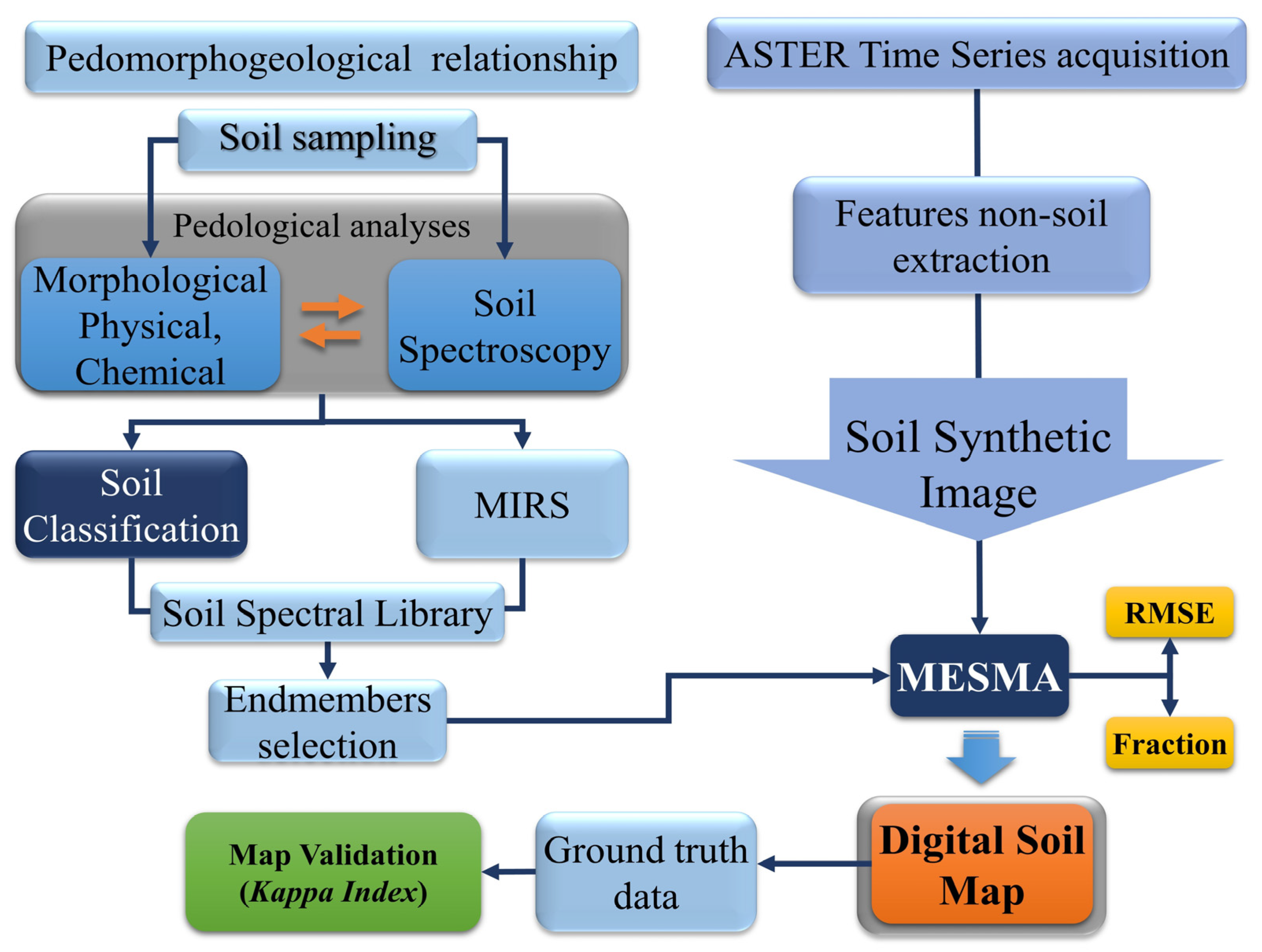
2. Materials and Methods

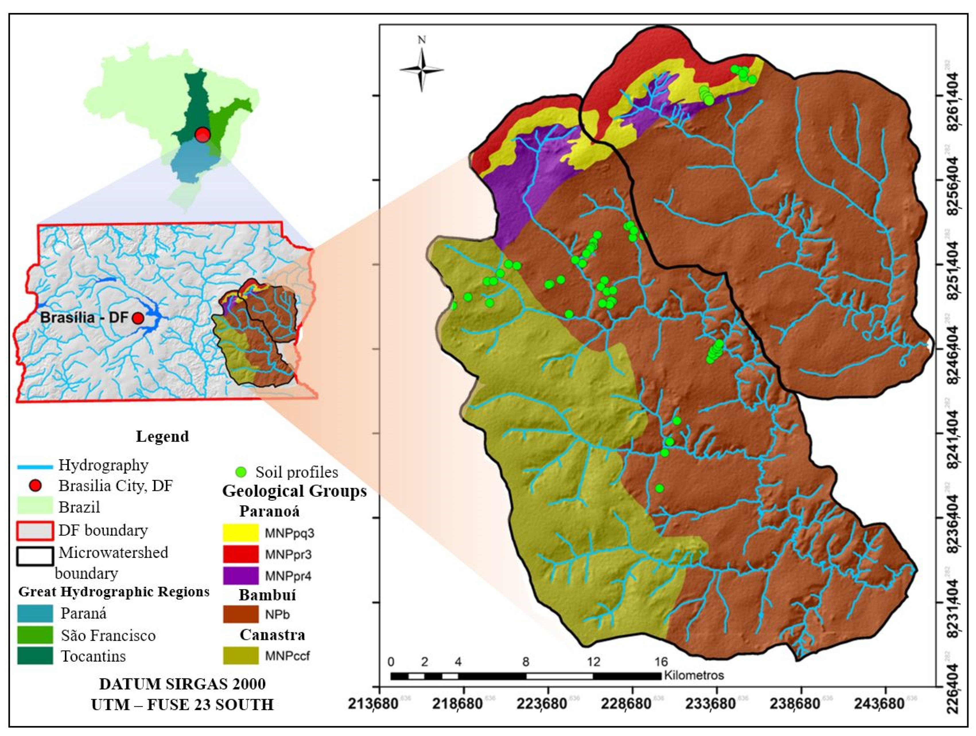
2.1. Study Area Characterization

The study area comprised two micro-watersheds, Rio Jardim (RJ–source area) and Ribeirão Extrema (RE–target area), with about 25,614 and 52.76 ha, respectively, of the Eastern Distrito Federal (DF) in UTM zone 23S coordinates: 213,680 m, 8,226,404 m, and 248,680 m 8,243,404 m, in Midwest Brazil (Figure 1). This area is on the Central Plateau geomorphological domain, developed over metasedimentary pelitic and psammitic rocks of the Paranoá, Canastra and Bambuí Groups, containing high levels of iron that gave reddish hues to the soils [20]. The soils are naturally acidic, with high aluminum contents and low exchangeable bases, which promote low natural fertility in local soils [10].
The physiographic conditions associated with a tropical climate favor the formation of highly weathered soils [10,16,21]. The Ferralsols cover most of the region in flat areas and at varying altitudes [22]. On slopes above 3%, Petric Plinthosols, which are associated with clayey Regosols, also occur. In a smaller proportion appear the Arenosols, Haplic Plinthsols, Cambisols, Argisols, Nitisols, Gleisols, and Histosols [10]. The pedological texture varies from very clayey to sandy, with high porosity (>50%) [10,21]. Most soils are acidic and dystrophic, a condition in which the exchangeable bases of the soil have almost all been leached so that Fe and Al sesquioxides remain basically [10,14,16,19].
The Cerrado (Savannah), in their various phytophysiognomies, covers part of the study area [23]. However, this region is characterized by intensive agricultural practices under a no-till system [2]. The region has a humid tropical climate with two well-defined seasons: rainy and hot in the summer (Aw) and dry in winter and Cwa, according to Köppen’s climatic classification, in which the annual rainfall average oscillates from 1200 to 1800 mm [24].

2.2. Fieldwork and Laboratory Activities

A general research workflow is shown in the Figure 2 to summarize the methods, which will be described in the subsequent sections.
Firstly, pedomorphogeological relationships were established in the study area following ref. [25], where 8 toposequences and 42 soil profiles were determined. The soil sampling occurred at an average depth of 0–15 cm in the surface layer and 20–100 cm in the subsurface layer for those soils that allowed the profile observation, following the ref. [26] recommendations. So, we performed pedological analyses, such as morphological (color), chemical (assortment complex, pH, and organic matter), and physical (texture) following ref. [26]. These steps were necessary for soil categorization in the Brazilian Soil Classification System [27] and correspondent classes at the World Reference Bases [1].
The reflectance of soil samples from surface horizons was obtained using the FieldSpec® Pro spectroradiometer, which has 2150 bands between 350 and 2500 nm (0.35 and 2.5 µm). Three readings were taken in different positions in which the electromagnetic radiation sensor stayed vertically oriented at 8 cm from the target, where the energy reflected the samples onto a plate, according to ref. [28]’s recommendations. The lighting source consists of two 50 W Quartz-Tungsten Halogen filament lamps, which are positioned 35 cm from the sample on reflective supports and are oriented 30 cm from the horizontal (angle of incidence). According to ref. [28], a white spectralon plate with more than 99% reflectance calibrated the equipment. The sensor was calibrated initially and every 20 min or 20 samples read, avoiding noise in the readings [18].

2.3. Soil Spectra Characterization

The morphological characterization of the soil spectra allows qualitative assessments based on the methods employed by ref. [18]. The qualitative analyses were carried out by observing the spectral curve’s specific features and pattern, including morphological characteristics, albedo intensity, shape aspects, general inclination, and curve inclination changes along the VNIR-SWIR spectral bands.
Afterward, hierarchical group analysis organized the spectral signatures according to the pedological class and, subsequently, the soil texture. We calculated the curve medians from the generated spectral soil classes. Thus, each endmember represented one pedological class near the study area, as performed by refs. [10,16]. The endmembers were transformed using a second derivative function of Kubelka-Munk to highlight the main soil features. Derivative spectra and soil attributes were analyzed using Pearson’s Correlation. Finally, a Soil Spectral Library (SSL) was developed with the resulting endmembers using the Spectral Library Builder application in ENVI 5.3. It was convolved into the eight first ASTER’s bands allocated into the VNIR and IR spectral ranges using ENVI software, as reported by ref. [4].

2.4. ASTER Digital Data Processing

Six images from the ASTER sensor were acquired during the dry season (from July to October) and covered the study area from the Earth Explorer digital platform (https://earthexplorer.usgs.gov/, accessed on 22 May 2022). During the dry season, there is low atmospheric moisture incidence and, consequently, a cloud cover smaller than 10%, increasing the sensor capacity in the soil spectral capitation. This capacity is favored in the study area due to the higher bare soil during the off-season crop [2], caused by the natural exposition of the soil surface in the drought season in the Savannah vegetation (Cerrado) [23]. The sensing period varied from July to November, 24 October 2001, 28 July 2004, and 20 September 2006. The ASTER products utilized were L1-B, processing level images with 8-bit radiometric resolution [11].
We acquired the following ASTER spectral bands: visible range B1 (green, 0.52–0.60 µm), B2 (red, 0.63–0.69 µm); Near Infrared B3N (NIR, 0.76–0.86 µm); and Shortwave Infrared (SWIR): B4 (SWIR 1, 1.60–1.70 µm), B5 (SWIR 2, 2.15–2.19 µm), B6 (SWIR 3, 2.19–2.23 µm), B7 (SWIR 4, 2.24–2.29 µm) and B8 (SWIR 5, 2.3–2.37 µm) [11].
We applied the FLAASH (Fast Line-of-Sight Atmospheric Analysis of Spectral Hypercubes) atmospheric correction to the ASTER images using the ENVI program version 5.4. Furthermore, the geometric and crosstalk effect corrections were performed as described in ref. [12]. The georeferencing of the images was supported by the stream and roads from the study area, following recommendations in ref. [11]. The ASTER SWIR bands (30 m of spatial resolution) were downscaled to 15 m to match the spatial resolution of the VNIR bands, according to ref. [4]. Subsequently, the images of the same date (2001, 2004, and 2006) were mosaicked into a single one, covering the entire study area.

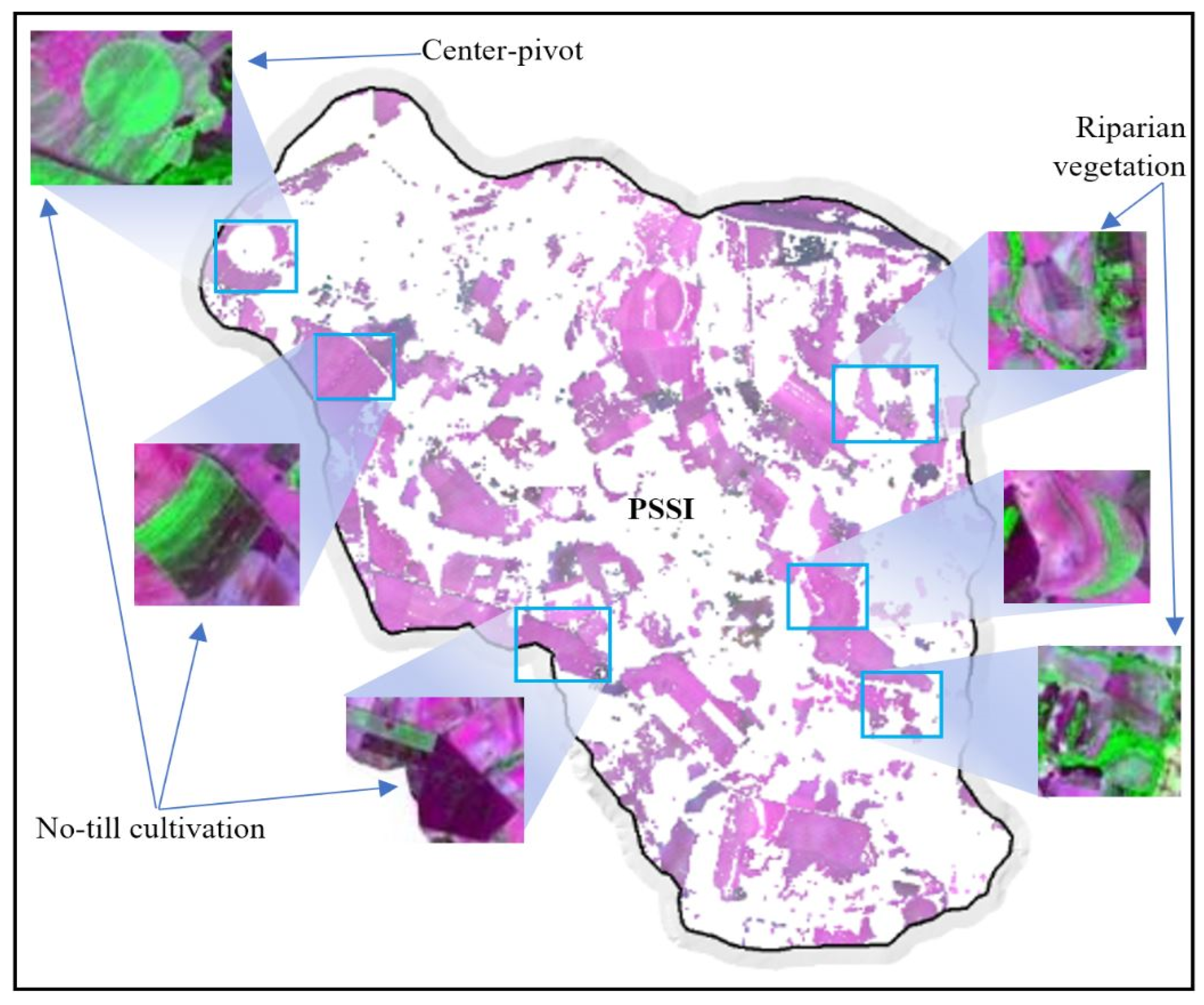
2.5. Bare Soil Image

The scenes’ non-soil features were masked by digital image processing combining spectral indices by conditional rules from threshold values of indices and quality images to classify exposed soil, according to [6,13,15]. The vegetation features were removed by the Normalized Difference Vegetation Index (NDVI) with values higher than 0.3. The NDVI was calculated according to Equation (1).
N D V I = ρ N I R ρ r e d ρ N I R + ρ r e d  
where, ρ N I R is the reflectance at Near-Infrared B3N (NIR, 0.76–0.86 µm) and ρ r e d corresponds to B2 (red, 0.63–0.69 µm) in the ASTER sensor system.
Features of water and burned areas were removed using the MAXVER classification algorithm (maximum likelihood). Straw features were extracted using the SINDRI index (Shortwave Infrared Normalized Difference Residue Index) according to ASTER bands, developed by Guy Serbin and collaborators [29], relating the SWIR intervals B6 and B7 to minimize crop residues on the soil spectral response (Equation (2)):
S I N D R I = B 6 B 7 B 6 + B 7
where, B6 and B7 are SWIR bands of the ASTER sensor.
Afterward, we built a mask using a band math function from ENVI with the following operation B4/{[2 (B4) + B5]/3}. This procedure standardized the effect of moisture on the soil surface to simulate the ASTER spectral range [30]. Finally, a soil mask was applied to each image to remove the non-soil features, which were then used to calculate the median values of the reflectance, resulting in a synthetical soil image (SySI) [13].

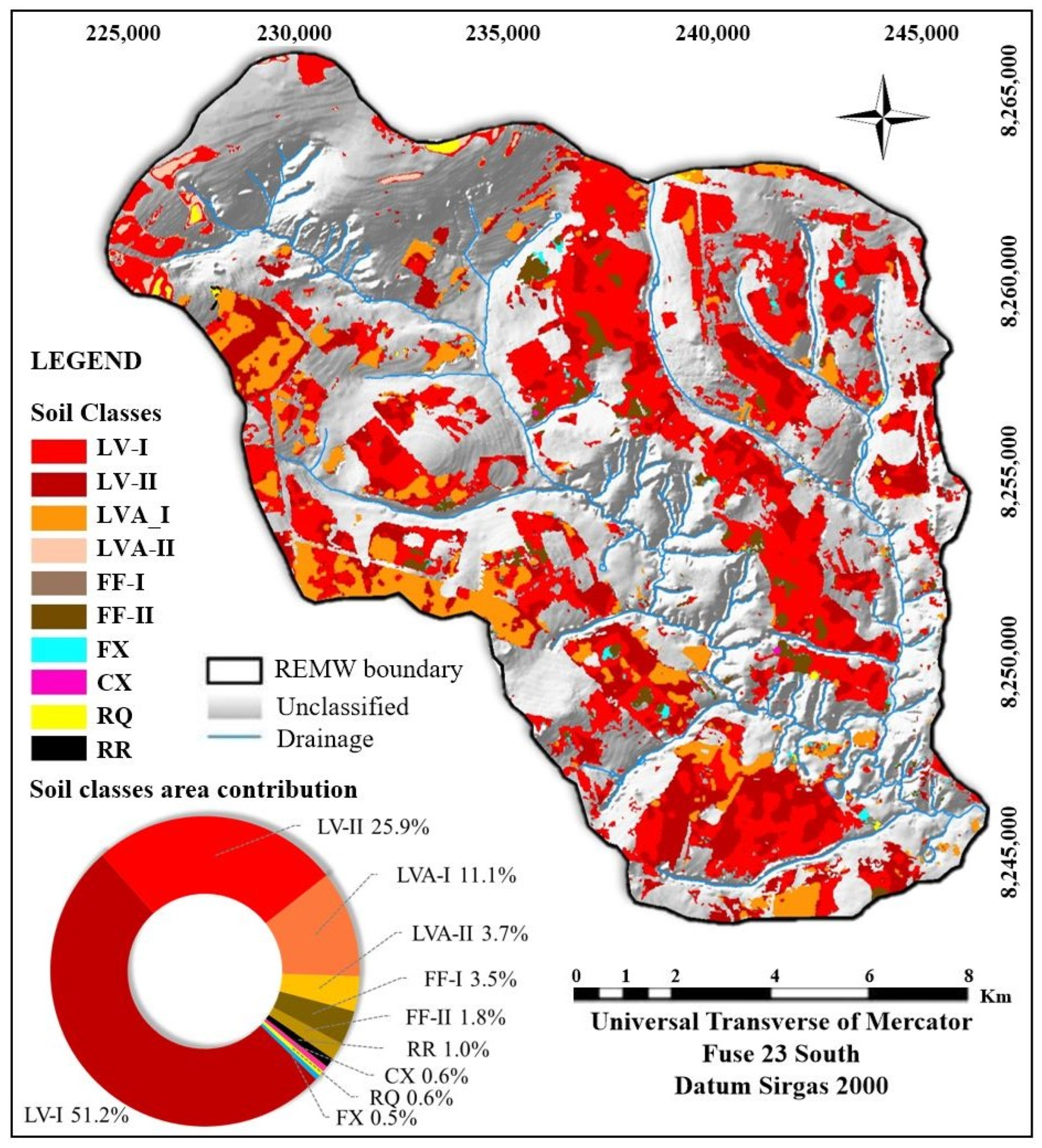
2.6. Digital Soil Mapping

The Multiple Endmember Spectral Mixture Analysis (MESMA), proposed by D. A. Roberts and other researchers [31], was applied using the soil endmembers and the SYSI to map the soil classes. The algorithm retuned three data types, namely: a fraction of modeled endmembers, an error image, and the spectral models’ images. It is noteworthy that we excluded the Gleisols and Histosols because they occurred in gap areas from the SySI. Therefore, these soil classes were not mapped but were described to represent the local pedodiversity.
The image with spectral unmixing models represents the soil classes identified by MESMA whose pixels are the highest proportion endmember. A median statistical convolution filter from a 5 × 5 size mask smoothed this data. Thus, the final map achieved a 15 m scale. Subsequently, the areas related to the spectral classification were calculated according to their corresponding endmembers. Finally, the models were labeled on the final map with contrasting colors based on ref. [27].

2.7. Digital Soil Map Validation

The accuracy of DSM occurred by checkering the errors and hits from points obtained in the field using a stratified 1100 × 1100 m grid, according to ref. [32]. The positions were determined randomly, according to each class area’s weight assignment. We utilized pedological data sources as field truth. They were obtained from Geoped’s soil database [10] with different locations of those points used in soil modeling. Afterward, we described the adopted procedures for hypothesis testing and discussion support.
It is noteworthy that those cells allocated to empty spaces in the grid were eliminated. Thus, only 161 points remained to continue in the validation process. The Kappa index assessed the mapping quality using the validation points, the user’s accuracy, the producer’s accuracy, and omission and commission errors, as ref. [32] recommended.

3. Results

3.1. Representative Soil Classes Description from the Study Area

During the surveying, 12 (Table 1) soil classes were found in the source and target areas, which were considered representative of the region’s pedodiversity, according to previous works [10,16,21]. We found Ferralsols, Plinthosols, Regosols and a few Cambisols, Arenosols, Gleisols, and Histosols, typical of tropical regions. besides, the soil texture provided an additional categorical level in the Brazilian System of Soil Classification [27].
In the Table 1, eleven profiles were classified as Dystric, Rhodic Ferralsol (LATOSSOLO VERMELHO Distrófico típico–LV), the texture ranged from very clayey (5 soil profiles) to clayey (6 soil profiles). Dystric, Haplic Ferralsol (LATOSSOLO VERMELHO-AMARELO Distrófico típico–LVA), four profiles presented clayey texture and the other four profiles presented loam-sandy. These textures were found only at RE (target area), formed from metarithmitics lithology, as observed in ref. [10]. The LV exhibited the 10R hue from Fe oxides–hematite predominant in LV and goethite in LVA (10YR) [16].
The Endopetric Plinthosol (PLINTOSSOLO PÉTRICO Concrecionário típico–FF), also presented two subtypes: four types with very clayey texture and four soils with clayey texture. Ref. [25] related a concretionary horizon occurrence inner profile of these soils in the DF’s High Plateaus, in which the water flow in the geomorphological edges alters the pedoenvironment. On the other hand, the Dystric Haplic Plinthosol (PLINTOSSOLO HÁPLICO Distrófico típico–FX) occurred only once, whose texture was clayey, showing redishes tones (10R 5/8) into horizon C to brownish (10YR 6/8) on horizon A, with horizons of variegated colors.
While the Dystric Regosols (NEOSSOLO REGOLÍTICO Distrófico típico–RR) presented in RJ (source area), six clayey texture profiles were observed. These soils showed an A horizon whose color ranged from dark reddish-brown (5YR 4/4) to reddish yellow (10YR 5/4) and from dark red (10R 3/6) to reddish yellow (2.5YR 6/8) in the C horizon, as described in ref. [16] in the RJ, the source area. Dystric Haplic Cambisol (CAMBISSOLO HÁPLICO Distrófico típico–CX) presented a clayey texture. According to Lacerda and Barbosa (2012), the soils developed from pelitic rocks of the Bambuí Group present colors ranging between 10 YR and 7.5 YR in horizons A and B, respectively. Two other profiles remaining represented the Dystric Arenosol (NEOSSOLO QUARTZARÊNICO Órtico típico–RQ). By definition, it is a sandy soil with low OM and iron oxides [10]. Its mineralogy predominantly consists of quartz, producing high reflectance intensity in the sand fraction [14].
Among soils with high organic matter (OM) content, the Dystric Haplic Gleysol (GLEISOLO HÁPLICO tb Distrófico típico–GX) occurred in two profiles presenting clayey texture, while Dystric Haplic Histosol (ORGANOSSOLO HÁPLICO Hêmico típico–OX) 275 occurred only in one profile, exhibiting clayey texture with less weathering and hydromorphic sedimentation, typical in these soils [1,27].

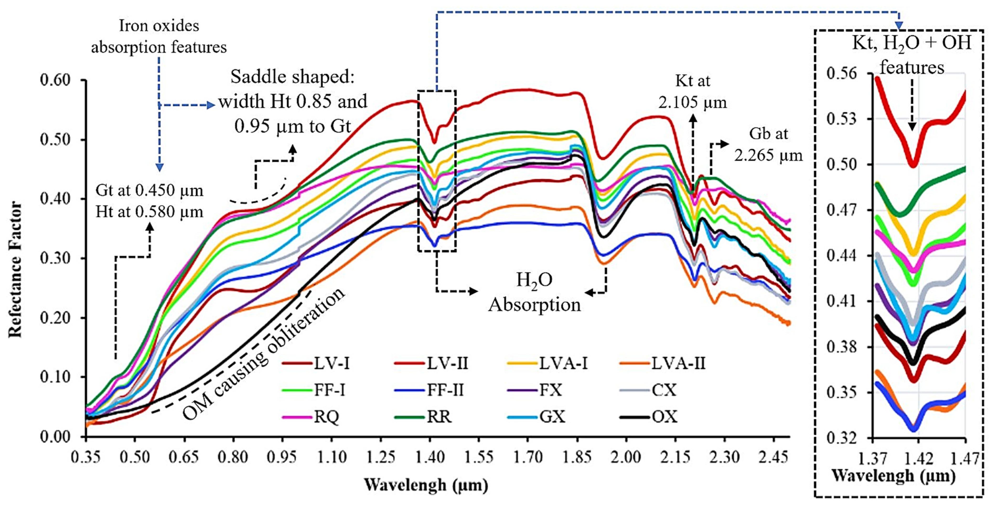
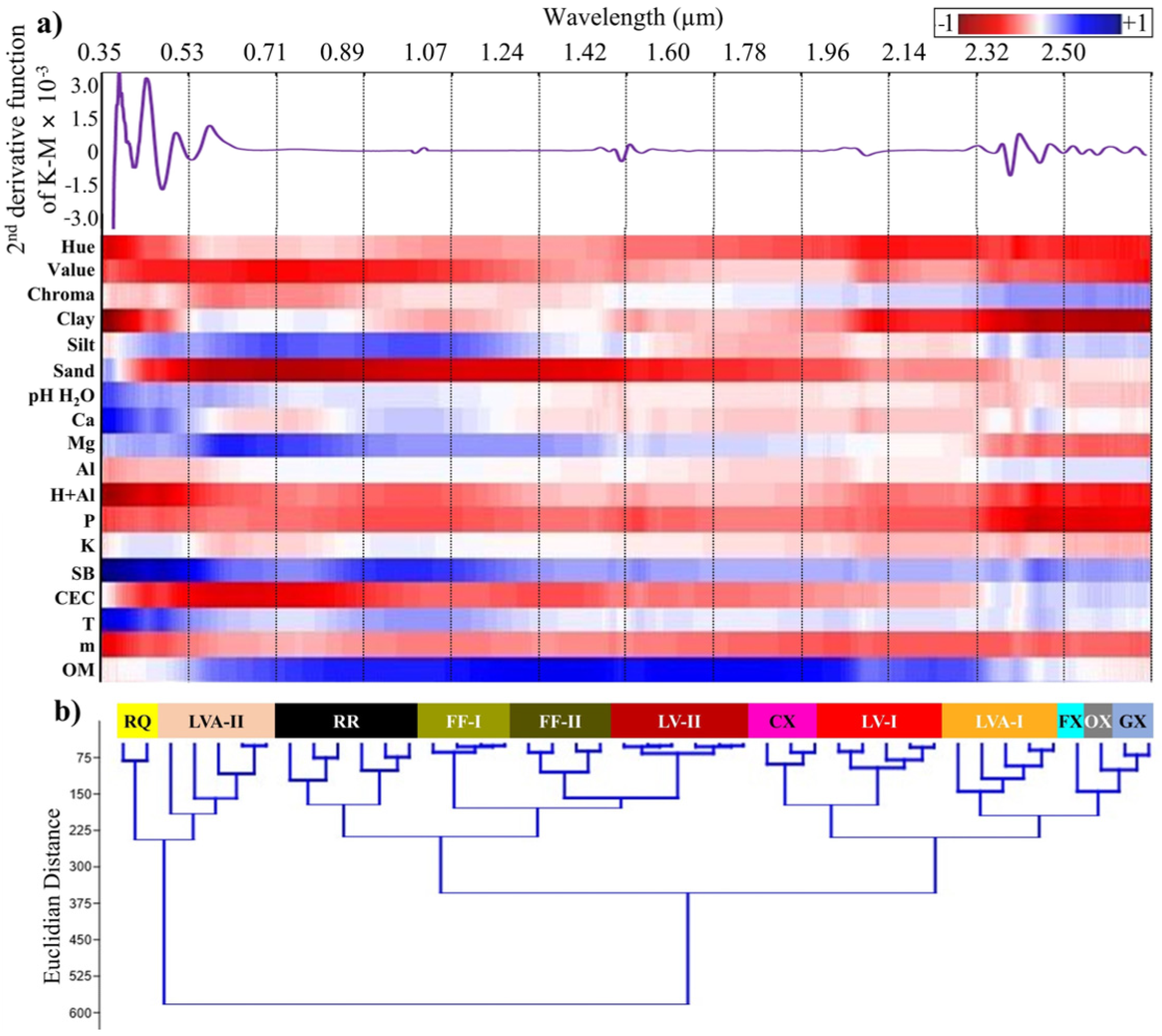
3.2. Spectral Patterns of Representative Soils

Figure 3 also shows the LVA (Haplic Ferralsol) spectra, which had eight samples, of which 4 represented LVA with a very clayey texture (LVA-I) from RJ (source area) that generated a median curve with a flattened aspect in the studied spectral range (0.35 to 2.5 µm). The LVA presented color 5YR due to the lower iron oxides or OM content and less clayey texture to obliterate the features [16]. Another four spectral signatures of the soils obtained in the northwest portion of RE (target area) represented the loam-sandy LVA (LVA-II). This curve’s highest intensity of the reflectance factor reached was 0.35, considered a low value for soils with a sandy texture, as stated by [19]. The Petric Plinthosols, represented by the acronym FF, are formed by two spectral classes: FF-I for clayey texture and FF-II for very clayey texture. These spectral curves showed a maximum reflectance factor of 0.35 in FF-I and 0.5 in FF-II. One grouping was defined for Haplic Plinthosols (FX) with a clay texture. The main features found in this soil were the iron oxides Gt and Ht, as also observed in ref. [10]. It presented a lower peak for the Gb feature and the hydroxyl group at 1.4, 1.9 (presence of 2:1 clay minerals), and 2.205 µm. The median spectrum of the soil class acronym RR (Regosols) showed a reflectance factor of 0.5. Despite being clayey soil, the content of more stable minerals such as quartz, particularly in the sand fraction, causes an increase in the RR soil reflectance. The spectral curve showed typical iron oxides’ characteristic absorption features, predominating Gt (0.48 and 0.9 µm), and a weak Kt at 2.205 µm, as shown in Figure 3.
The two GX (Gleisol) profiles analyzed generated one spectral class of clay texture. The reflectance factor’s maximum values were 0.5, with a strong influence from the OM between 0.35 and 1.3 µm. The ascending shape of the spectral curve, such as that of GX associated with weak oxide features in these soils, is characteristic of hydromorphism. Only one sample of the OX class was represented in this work [10]. Its spectral curve showed low reflectance in the VIS due to high OM contents, producing a flat to concave shape (see Figure 3 above). According to refs. [10,16], the SWIR features can reveal some 2:1 mineral characteristics and Gb, indicating a lower evolution degree.
The Cambisol (CX) was represented by a single spectral grouping from three representative samples of the class. This endmember reached the maximum intensity of the soil reflectance factor of 0.45 and had typical iron oxide features, hydroxyls, and the implications of the effects of OM, and its shape was similar to LVA (Figure 3). Finally, the RQ showed absorption regions of 1.4 and 1.9 µm, less intense due to the quartz hygroscopic effect. This soil class differed spectrally more from the others, agreeing with [19] findings. A high albedo was also observed from the low content of iron oxides, opaque minerals, sandy texture, low OM content, and the presence of quartz.

3.3. Endmembers Organization

The intraclass textural differences served as criteria for spectral grouping due to their effect on variation spectra. Thus, Pearson’s correlation demonstrates high correspondence with most soil attributes throughout the reflectance spectrum at all wavelengths (Figure 4a). The clay and sand contents mainly exhibited a high negative correlation in VNIR and SWIR ranges. Therefore, based on the clay content, the clustering analysis enabled 12 spectral subgroups, generating a dendrogram and Euclidean distance index with 0.79 correlation (Figure 4b).
The soil spectra resulted in 10 endmembers representative of local pedodiversity (except Histosols and Gleisols). It is worth mentioning that this analysis was carried out considering the taxonomic soil classes that are represented in Figure 4b by their acronyms, according to the Brazilian Soil Classification System [27] (see Table 1 in Section 3.1 for compatibility with the WRB-FAO System [1]).
These results are similar to those obtained in ref. [16], who modeled soils using color as a base attribute for clustering analysis in the RJ region, here it was utilized as the source area. Another study [10] utilized texture for endmember grouping in the same area and stated that pedological attributes could cluster the soil classes.

4. Discussion

4.1. Soil Synthetic Image Assessment

The methodology for extracting bare soil features from the single images in the time series (2001, 2004, and 2009) was responsible for removing 60.30% of the RE (target area). These areas without information correspond mainly to the areas covered by vegetation in their various phenological stages. On the other hand, the 2006’ image was responsible for more than 60% of the SySI contribution, as shown in Table 2. Therefore, the bare soil image covered only 39.7% of the target area. This low number was attributed to the use of a short imaging period from the ASTER orbital sensor [11], as well as to land use and land cover dynamics, which covered the soil during most of the time series.
Observing Figure 5, it is possible to identify the bare soil areas captured by method GEOS3 [13], which produced a Synthetic Soil Image (SySI), pointing out typical colors for soil exposure in the combinations of these spectrum bands. The number of pixels and areas with bare soil were adequately calculated and arranged in Table 2. The SySI covered 10,168 ha, 40% of the same area, with pixels representing bare soils using Land Sat imagery. The researchers cited in ref. [6] obtained 53% of bare soil covering with ASTER, and ref. [13] achieved 68%, both in São Paulo, Southern Brazil. Finally, ref. [33] achieved 100% of the soil image using kriging and cloud-based processing of LandSat data in a large area of the Brazilian Midwest over a 30-year time series.
The angular-shaped patterns are easily identifiable in the SySI and typical of areas occupied by crops. The high-intensity agricultural activities confer areas with polygonal shapes (Figure 5 above). Furthermore, the no-till cultivation system has low soil disturbance and crop residues’ keeping on the soil surface (straw in decomposition) [23]. These results showed that although the ASTER sensor no longer acquires data in the infrared range, its legacy data is still helpful for environmental modeling.

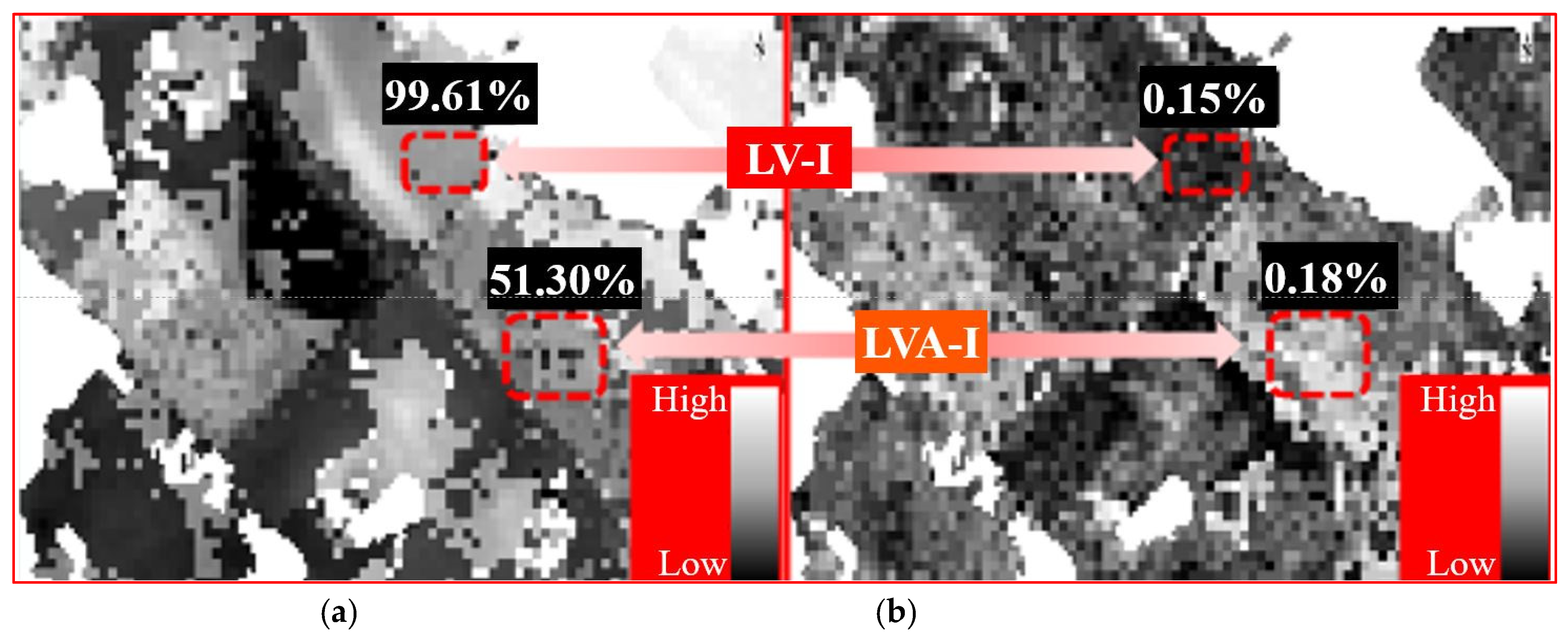
4.2. Spectral Mixture Analysis Model with Multiples Endmembers (MESMA)

The soil classes classified as LV (Rhodic Ferralsols) predominate in the study area (Table 3). According to our modeling, these soils occupied a total area of 7846 ha. Second, there is the LVA (Haplic Ferralsols), which covers an area of 1604 ha. These areas obtained from LV and LVA follow the region surveying carried out by ref. [21] on a scale of 1:100,000, which stated that Ferralsols cover 77% of the study area.
Table 3 also exhibits other soil classes with lower mapped areas, in which: 545 ha are assigned to FF, 30 ha to RR, 44 ha to CX, and 51 ha to FX. The low frequency of these classes of soils in the mapping carried out can be explained by developing more restricted areas in the target area with more steep slopes, which were excluded in the SySI processing. It is noteworthy mentioning the similarity of the soil classes FF and LVA spectra reported by [10]. These characteristics make the model mismatch since both spectra have a latossolic matrix, a feature typical of Ferralsols [19].
The algorithm modeled the pixels in a fraction image for each endmember demixed in the SySI in shades of gray, in which the lighter shade represents a greater probability of occurrence for the endmember (Figure 6a). These presented a root mean square error (RMSE) (Figure 6b) concerning the pixel’s spectral curve. In this study, the RMSE, or mean square error of the MESMA model, was 1.02%. Roberts et al. (1998) [31] stated that a suitable RMSE value should not exceed 2.5%. Despite crosstalk corrections, the spectral curves in the ASTER imagery were strongly damaged, modifying the spectral curves [12], hence this was considered the principal reason for higher RMSE values.
The soil classes’ distribution and arrangement throughout the study area reveal that the DSM (Figure 7) achieved its objective satisfactorily. The hillshade effect supported the soil arrangement observation, highlighting the weathered soils’ predominance in flat regions and less evolved soils where the relief was irregular. The soil classes mapped represented 39.7% of the RE (target area), corresponding to about 10.2 ha. This area was considered satisfactory due to the short time series achieved with the methodology adopted for mapping bare soils in this research, agreeing with ref. [13].
We observed occasional occurrences of Plinthosols (FF and FX) in the residual hills of the landscape. Their spatial representation decreases towards the downstream of the RE. These soil classes evidence the linking with erosive and pedogenetic processes towards the Rio Preto watershed. It is noteworthy that the Embrapa mapping from the 1970s did not include the soil classes FF and RR (Plinthosols and Regosols, respectively), nor did it after its updating by ref. [21]. Despite our map including the FF and RR soil classes, it does not show these classes, due to the spatial resolution and the suppression of areas during the map production that do not allow such observations. Thus, these soils were generalized. On the other hand, the DSM made in this work presented the particular distribution as verified infield for soils classes FF and RR. The RRs usually occur in the drainage fitting when the slope accentuates abruptly, because this the OM is lacking [22].

4.3. Digital Soil Classes Map Validation

The DSM evaluation generated in the RE watershed carried out by analyzing the error matrix with 161 validation points, presented a Kappa index of 0.73 or 73% (Table 4). This mapping’s global accuracy obtained “very good” performance [32]. Several studies on digital soil mapping based on other DSM techniques have shown variations in the Kappa index.
Some researchers achieved similar results. For instance, ref. [6] mapped soil attributes in São Paulo state, Brazil, using the MESMA, and they reached a Kappa index of 63%. The mapping performed by refs. [10,16] reached a Kappa index of 0.73 and 0.75, respectively, in the eastern part of the Brazilian Federal District. Comparing our results with other techniques from a literature review about DSM in Brazil carried out by [34], whose stated average Kappa values were around 48% for pedometric maps.
Soil class according to Brazilian Soil Classification System [27], see Table 1 for classes correspondence according World Reference Base for soil research [1]. UA: User’s Accuracy, PA: Producer’s Accuracy, OE: Omission Error, CE: Commission Error, a: LATOSSOLO VERMELHO Distrófico típico muito argiloso (LV-I); b: LATOSSOLO VERMELHO Distrófico típico argiloso (LV-II); c: LATOSSOLO VERMELHO-AMARELO Distrófico típico muito argiloso (LVA-I); d: LATOSSOLO VERMELHO-AMARELO Distrófico típico franco-arenoso (LVA-II); e: PLINTOSSOLO PÉTRICO Concrecionário distrófico muito argiloso (FF-I); f: PLINTOSSOLO PÉTRICO concrecionário distrófico argiloso (FF-II); g: NEOSSOLO REGOLÍTICO distrófico argiloso (RR); h: CAMBISSOLO HÁPLICO tb distrófico argiloso (CX); i: NEOSSOLO QUARTZARÊNICO Órtico típico distrófico (RQ) and j: PLINTOSSOLO HÁPLICO Distrófico típico argiloso (FX).

4.4. Limitations and Perspectives

Given the data obtained and the discussion raised, we describe the main technical limitations of the method so that future work can be explored to circumvent such limitations. The first problem concerns the sensor adopted for the study, as it has been out of operation in the infrared range since 2008 [12]. This factor limits the study to more stable targets, such as soil and rocks, to the detriment of monitoring dynamic targets, such as vegetation, water, and burned areas. We suggest using another orbital sensor to include these data as covariates in a machine learning model, for example, as performed by [33]. Secondly, the short time series did not allow us to extract all soil features altered by surface moisture, even by applying the index proposed here. A more extended time series could normalize these data through geoprocessing techniques, including cloud-based Remote Sensing data [10].
Another point is related to data quality. New studies may test the strategy in areas farther from the field data collection point. Moreover, we infer that the results will be better as soil surface information associated with subsurface characteristics that determine soil classification is included, e.g., Plinthosols and Ferralsols differentiation, as related by ref. [10]. In this sense, the use/development of pedotransfer algorithms that relate the characteristics of the topsoil (water holding capacity or land use and land cover) with the subsoil characteristics of interest (slope, aspect, geology) or the characteristics that are significantly influenced by their presence, they can help in the classification since different soils are formed under the same conditions.
Finally, we cite the low amount of data collected and the proximity of the target area, which may have biased the results. Therefore, expert integration of all these potential indicators of subsurface soil properties along with subsurface observations is needed to extrapolate and create maps for distant locations and compare them to legacy maps. On the other hand, since soil classification is often based on arbitrary ranges of certain subsurface features, it will be challenging to determine the extent of specific pedological categories without sufficient information collected in the soil profile.

5. Conclusions

Spectral modeling of a satellite bare soil image using laboratory endmembers and the MESMA method resulted in an accurate (Kappa index of 0.73) pedological map. Therefore, proximal and remote sensing data can provide detailed digital soil mapping with “very good” accuracy, according to the map quality.
Similar physiographic and geological characteristics can minimize modeling errors for spectral data extrapolation. However, other information, such as vegetation and hydric aspects, must be included in the modeling.
Furthermore, the legacy ASTER data can still be used to model the environment, although it does not acquire more data in the infrared range. Other sensors that include a higher spectral resolution, such as Sentinel-1, or more significant legacy imaging, such as the Landsat series sensors, can improve this technique by increasing the quality of the data modeled.

Author Contributions

Conceptualization, J.J.N., R.R.P., M.P.C.L. and J.A.M.D.; data curation, J.J.N., R.R.P. and J.A.M.D.; formal analysis, J.J.N.; funding acquisition, J.J.N., R.R.P., M.P.C.L. and J.A.M.D.; investigation, J.J.N. and R.R.P.; methodology, J.J.N., R.R.P. and J.A.M.D.; project administration, J.J.N., M.P.C.L., R.R.P. and M.P.O.J.; resources, J.J.N., M.P.C.L., J.A.M.D. and R.R.P.; software, R.R.P., J.J.N. and J.A.M.D.; supervision, M.P.C.L. and J.A.M.D.; validation, J.J.N., M.P.C.L. and M.P.O.J.; visualization, J.J.N. and R.R.P.; writing—original draft, J.J.N.; Writing— review and editing, J.J.N. and R.R.P. This article is part of a Ms. D. research project conducted by the first author under the supervision of the second and third authors. All authors have read and agreed to the published version of the manuscript.

Funding

This research was funded by the Coordination for the Improvement of Higher EducationPersonnel (Coordenação de Aperfeiçoamento de Pessoal do Ensino Superior—CAPES) (MS.D. scholarship, grant #88882.383908/2019-01). The Federal District Research Support Foundation (Fundação de Apoio à Pesquisa do Distrito Federal—FAP/DF): official notice 16733.78.29498.26042017. And the São Paulo State Research Support Foundation (Fundação de Apoio à Pesquisa do Estado de São Paulo – FAPESP): process number 2014/22262-0.

Data Availability Statement

The dataset related to physical, chemical, morphological and spectral soil analyses, as well as the shapefiles archives generated in this study are available on request directly from the first and second authors or Geoprocessing and Pedomorphology Laboratory—Geoped (geoped.unb@gmail.com).

Acknowledgments

The first author thanks the co-author for fieldwork and laboratory analyses assisting, methodological and theoretical support. Acknowledgments to the supervisors, particularly the fourth author on behalf of the Geotechnologies in Soil Science group (GeoCiS, https://esalqgeocis.wixsite.com/english, accessed on 18 January 2022) from ESALQ/ University of São Paulo, spectral readings and methodology teaching. It is worth thanking the Coordination for Improvement of Higher Education Personal (CAPES) and the Faculty of Agronomy and Veterinary Medicine from the University of Brasília–UnB for financial support and providing structure. In advance, we thank the editors and anonymous revisors who contribute to this text improvement.

Conflicts of Interest

The authors declare no conflict of interest.

References

  1. IUSS Working Group WRB; FAO; IUSS Working Group WRB. World Reference Base for Soil Resources 2014 International Soil Classification System; World Soil Resources Reports No. 106; FAO: Rome, Italy, 2015; ISBN 9789251083697. [Google Scholar]
  2. Novais, J.J.; Lacerda, M.P.C. Sentinel-2 imagery usage on environmental monitoring of land use and occupation in a microwatershed in Central Brazil. Gaia Sci. 2021, 15, 76–92. [Google Scholar] [CrossRef]
  3. Minasny, B.; McBratney, A.B. Digital soil mapping: A brief history and some lessons. Geoderma 2016, 264, 301–311. [Google Scholar] [CrossRef]
  4. Genú, A.M.; Roberts, D.; Demattê, J.A.M. The use of multiple endmember spectral mixture analysis (MESMA) for the mapping of soil attributes using ASTER imagery. Acta Sci. Agron. 2013, 35, 377–386. [Google Scholar] [CrossRef] [Green Version]
  5. Nawar, S.; Buddenbaum, H.; Hill, J.; Kozak, J. Modeling and mapping of soil salinity with reflectance spectroscopy and landsat data using two quantitative methods (PLSR and MARS). Remote Sens. 2014, 6, 10813–10834. [Google Scholar] [CrossRef] [Green Version]
  6. Gallo, B.C.; Demattê, J.A.M.; Rizzo, R.; Safanelli, J.L.; de Mendes, W.S.; Lepsch, I.F.; Sato, M.V.; Romero, D.J.; Lacerda, M.P.C. Multi-temporal satellite images on topsoil attribute quantification and the relationship with soil classes and geology. Remote Sens. 2018, 10, 1571. [Google Scholar] [CrossRef]
  7. Diek, S.; Schaepman, M.E.; de Jong, R. Creating multi-temporal composites of airborne imaging spectroscopy data in support of digital soil mapping. Remote Sens. 2016, 8, 906. [Google Scholar] [CrossRef] [Green Version]
  8. Rogge, D.; Bauer, A.; Zeidler, J.; Mueller, A.; Esch, T.; Heiden, U. Building an exposed soil composite processor (SCMaP) for mapping spatial and temporal characteristics of soils with Landsat imagery (1984–2014). Remote Sens. Environ. 2018, 205, 1–17. [Google Scholar] [CrossRef] [Green Version]
  9. Chabrillat, S.; Ben-Dor, E.; Cierniewski, J.; Gomez, C.; Schmid, T.; van Wesemael, B. Imaging Spectroscopy for Soil Mapping and Monitoring. Surv. Geophys. 2019, 40, 361–399. [Google Scholar] [CrossRef] [Green Version]
  10. Novais, J.J.; Lacerda, M.P.C.; Sano, E.E.; Demattê, J.A.M.; Oliveira, M.P. Digital soil mapping by multispectral modeling using cloud-computed landsat time series. Remote Sens. 2021, 13, 1181. [Google Scholar] [CrossRef]
  11. Abrams, M.; Hook, S.; Ramachandran, B. Aster User Handbook, 2nd ed.; Technology Institute: Foster City, CA, USA, 2007; Volume 2. [Google Scholar]
  12. de Baptista, G.M.M.; Vivaldi, D.D.; Meneses, P.R. Correção atmosférica e de “crosstalk” em dados Aster para mapeamento da relação mineralógica de solos. Pesqui. Agropecu. Bras. 2016, 51, 1272–1282. [Google Scholar] [CrossRef]
  13. Demattê, J.A.M.; Fongaro, C.T.; Rizzo, R.; Safanelli, J.L. Geospatial Soil Sensing System (GEOS3): A powerful data mining procedure to retrieve soil spectral reflectance from satellite images. Remote Sens. Environ. 2018, 212, 161–175. [Google Scholar] [CrossRef]
  14. Poppiel, R.R.; Lacerda, M.P.C.; Demattê, J.A.M.; Oliveira, M.P.; Gallo, B.C.; Safanelli, J.L. Pedology and soil class mapping from proximal and remote sensed data. Geoderma 2019, 348, 189–206. [Google Scholar] [CrossRef]
  15. Demattê, J.A.M.; Safanelli, J.L.; Poppiel, R.R.; Rizzo, R.; Silvero, N.E.Q.; de Mendes, W.S.; Bonfatti, B.R.; Dotto, A.C.; Salazar, D.F.U.; Mello, F.A.d.O.; et al. Bare Earth’s Surface Spectra as a Proxy for Soil Resource Monitoring. Sci. Rep. 2020, 10, 4461. [Google Scholar] [CrossRef] [PubMed] [Green Version]
  16. Poppiel, R.R.; Lacerda, M.P.C.; Demattê, J.A.M.; Oliveira, M.P.; Gallo, B.C.; Safanelli, J.L. Soil class map of the Rio Jardim watershed in Central Brazil at 30 m spatial resolution based on proximal and remote sensed data and MESMA method. Data Br. 2019, 25, 104070. [Google Scholar] [CrossRef]
  17. Coblinski, J.A.; Giasson, É.; Demattê, J.A.M.; Dotto, A.C.; Costa, J.J.F.; Vašát, R. Prediction of soil texture classes through different wavelength regions of reflectance spectroscopy at various soil depths. Catena 2020, 189, 104485. [Google Scholar] [CrossRef]
  18. Demattê, J.A.M.; Bellinaso, H.; Romero, D.J.; Fongaro, C.T. Morphological Interpretation of Reflectance Spectrum (MIRS) using libraries looking towards soil classification. Sci. Agric. 2014, 71, 509–520. [Google Scholar] [CrossRef]
  19. Lacerda, M.P.C.; Demattê, J.A.M.; Sato, M.V.; Fongaro, C.T.; Gallo, B.C.; Souza, A.B. Tropical texture determination by Proximal Sensing using a regional spectral library and its relationship with soil classification. Remote Sens. 2016, 8, 701. [Google Scholar] [CrossRef] [Green Version]
  20. Freitas-Silva, F.H.; Campos, J.E.G. Geologia do Distrito Federal. In Inventário Hidrogeológico e dos Recursos Hídricos Superficiais do Distrito Federal; Distrito Federal: Brasília, Brazil, 1998; Volume 1, 86p. [Google Scholar]
  21. Reatto, A.; Martins, E.S.; Farias, M.F.R.; Silva, A.V.; Carvalho Júnior, O.A. Mapa Pedológico Digital: SIG Atualizado do Distrito Federal Escala 1:100.000 e uma Síntese do Texto Explicativo, 120th ed.; Embrapa Cerrados—CPAC: Planaltina-DF, Brasil, 2004; ISBN 1517-5111. [Google Scholar]
  22. Lacerda, M.P.C.; Barbosa, I.O. Soil-Geomorphological relationships and pedoforms distribution in the ecological station of Águas Emendadas, Distrito Federal. Rev. Bras. Cienc. do Solo 2012, 36, 709–722. [Google Scholar] [CrossRef] [Green Version]
  23. Sano, E.E.; Rodrigues, A.A.; Martins, E.S.; Bettiol, G.M.; Bustamante, M.M.C.; Bezerra, A.S.; Couto, A.F.; Vasconcelos, V.; Schüler, J.; Bolfe, E.L. Cerrado ecoregions: A spatial framework to assess and prioritize Brazilian savanna environmental diversity for conservation. J. Environ. Manag. 2019, 232, 818–828. [Google Scholar] [CrossRef]
  24. Alvares, C.A.; Stape, J.L.; Sentelhas, P.C.; De Moraes Gonçalves, J.L.; Sparovek, G. Köppen’s climate classification map for Brazil. Meteorol. Zeitschrift 2013, 22, 711–728. [Google Scholar] [CrossRef]
  25. Barbosa, I.O.; Lacerda, M.P.C.; Bilich, M.R. Soils distribution model based on relation between geology, geomorphology and pedology, at the High Plateau of Distrito Federal, Brazil. Rev. Asoc. Geol. Argent. 2010, 66, 569–575. Available online: http://www.scielo.org.ar/pdf/raga/v66n4/v66n4a16.pdf (accessed on 18 January 2022).
  26. Burt, R. Soil Survey Staff Soil Survey Field and Laboratory Methods Manual. United States Dep. Agric. Nat. Resour. Conserv. Serv. 2014, 486. [Google Scholar] [CrossRef]
  27. Santos, H.G. Sistema Brasileiro de Classificação de Solos; Embrapa: Brasília, Brazil, 2018; ISBN 978-85-7035-198-2. [Google Scholar]
  28. ASD Inc. ASD Fieldspec® 4: The Industry-Leading Portable Device for Field Spectroscopy, 6th ed.; Analytical Spectral Device Inc.: Malvern, UK, 2019; 8p. [Google Scholar]
  29. Serbin, G.; Daughtry, C.S.T.; Hunt, E.R.; Reeves, J.B.; Brown, D.J. Effects of soil composition and mineralogy on remote sensing of crop residue cover. Remote Sens. Environ. 2009, 113, 224–238. [Google Scholar] [CrossRef]
  30. Novais, J.J. Digital Soil Mapping of the Ribeirão Extrema Watershed, Distrito Federal, from Multitemporal ASTER Images and Spectral Library; Graduate Program in Agronomy; Novais, J.J., Ed.; Faculty of Agronomy and Veterinary Medicine—FAV, University of Brasilia: Brasília-DF, Brasil, 2017. [Google Scholar]
  31. Roberts, D.A.; Gardner, M.; Church, R.; Ustin, S.; Scheer, G.; Green, R.O. Mapping chaparral in the Santa Monica Mountains using multiple endmember spectral mixture models. Remote Sens. Environ. 1998, 65, 267–279. [Google Scholar] [CrossRef]
  32. Congalton, R.G.; Green, K. Assessing the Accuracy of Remotely Sensed Data Principles and Practices, 2nd ed.; CRC Press/Taylor & Francis Group: Boca Raton, FL, USA; London, UK; New York, NY, USA, 2013. [Google Scholar]
  33. Poppiel, R.R.; Lacerda, M.P.C.; Safanelli, J.L.; Rizzo, R.; Oliveira, M.P.; Novais, J.J.; Demattê, J.A.M. Mapping at 30 m resolution of soil attributes at multiple depths in midwest Brazil. Remote Sens. 2019, 11, 2905. [Google Scholar] [CrossRef]
  34. Ten Caten, A.; Dalmolin, R.S.D.; Ruiz, L.F.C.; De Lourdes Mendonça-Santos, M. Digital soil mapping: Strategy for data pre-processing. Digit. Soil Assess. Beyond-Proc. Fifth Glob. Work. Digit. Soil Mapp. 2012, 36, 193–196. [Google Scholar]
Figure 1. Location map of Rio Jardim (RJ–source area) and Ribeirão Extrema (RE–target area), The green light dots represent the soil profile sampled spots. both overlaid with local geology, according to Freitas-Silva and Campos (1998) [20]. MNP: Mesoneoproterozoic age rocks (units: pq3–quartizite; pr3–rithmite; pr4–clay rithmite; b–bambuí; ccf–canastra).
Agriengineering 05 00011 g001
Figure 2. Methodology’s flowchart. MIRS: Morphological Interpretation Reflectance Spectrum; MESMA: Multiple Endmember Spectral Mixture Analysis; RMSE: Root Mean Square Error.
Agriengineering 05 00011 g002
Figure 3. Spectral library with the endmembers in the studied region, highlighting the following absorption features: Kt feature at 1.40 µm and organic material effect on OX spectra. Other features also are pointed, such as Ht: Hematite, Gt: Goethite, Kt: Kaolinite, Gb: Gibbsite.
Agriengineering 05 00011 g003
Figure 4. Data statistical analyzing: (a) Pearson’s correlation between soil attributes and different wavelengths of medium spectra; (b) Hierarchical clustering analysis by Euclidean distance similarity index based on texture (clay content). Where: Ca = Calcium, Mg = Magnesium, Al = Aluminium, P = Phosphorus, K = Potassium, SB = Sum of Bases, CEC = Cation Exchange Capacity, T = Bases Saturation, M = Aluminium Saturation, OM = Organic Matter; LV-I: LATOSSOLO VERMELHO Distrófico típico muito argiloso, LV-II: LATOSSOLO VERMELHO Distrófico típico argiloso; LVA-I: LATOSSOLO VERMELHO-AMARELO Distrófico típico muito argiloso; LVA-II: LATOSSOLO VERMELHO-AMARELO Distrófico típico franco-arenoso; FF-I: PLINTOSSOLO PÉTRICO Concrecionário distrófico muito argiloso; FF-II: PLINTOSSOLO PÉTRICO concrecionário distrófico argiloso; RR: NEOSSOLO REGOLÍTICO distrófico argiloso; CX: CAMBISSOLO HÁPLICO tb distrófico argiloso; RQ: NEOSSOLO QUARTZARÊNICO Órtico típico distrófico and FX: PLINTOSSOLO HÁPLICO Distrófico típico argiloso.
Agriengineering 05 00011 g004
Figure 5. Synthetic Soil Image from the study area outstanding the natural vegetation and agricultural features in the ASTER single images.
Agriengineering 05 00011 g005
Figure 6. Illustrative values of endmember fraction modeled (a) and Root Mean Square Error (b) for models LV-I (LATOSSOLO VERMELHO Distrófico típico muito argiloso–Rhodic Ferralsol) and LVA-I: LATOSSOLO VERMELHO-AMARELO Distrófico típico muito argiloso–Haplic Ferralsol).
Agriengineering 05 00011 g006
Figure 7. Digital soil classes map of the Ribeirão Extrema microwatershed (RE) with a pie chart showing the contribution percentage of soil classes to the mapped area. LV-I: LATOSSOLO VERMELHO Distrófico típico muito argiloso; LV-II: LATOSSOLO VERMELHO Distrófico típico argiloso; LVA-I: LATOSSOLO VERMELHO-AMARELO Distrófico típico muito argiloso; LVA-II: LATOSSOLO VERMELHO-AMARELO Distrófico típico franco-arenoso; FF-I: PLINTOSSOLO PÉTRICO Concrecionário distrófico muito argiloso; FF-II: PLINTOSSOLO PÉTRICO concrecionário distrófico argiloso; RR: NEOSSOLO REGOLÍTICO distrófico argiloso; CX: CAMBISSOLO HÁPLICO tb distrófico argiloso; RQ: NEOSSOLO QUARTZARÊNICO Órtico típico distrófico and FX: PLINTOSSOLO HÁPLICO Distrófico típico argiloso.
Agriengineering 05 00011 g007
Table 1. Brazilian and worldwide soil classification system of the study area.
1 SiBCS2 FAO3 Tex.4 Obs.5 EM.Origin
LATOSSOLO VERMELHO
Distrófico típico
Dystric Rhodic Ferralsolclayey5LV-IRJ
very-
clayey
6LV-IIRJ
LATOSSOLO VERMELHO-AMARELO Ditrófico típicoDystric Haplic Ferralsolclayey4LVA-IRJ
loam-
sandy
4LVA-IIRE
PLINTOSSOLO PÉTRICO
Concrecionário típico
Dystric Endopetric Plinthosolclayey4FF-IRJ
very-clayey4FF-IIRJ
PLINTOSSOLO HÁPLICO
Distrófico típico
Dystric Haplic Plintosolclayey1FXRJ
NEOSSOLO REGOLÍTICO
Distrófico típico
Clayic Dystric Regosolclayey6RRRJ
GLEISSOLO HÁPLICO
tb distrófico típico
Dystric Haplic Gleysolclayey2GXRJ
ORGANOSSOLO HÁPLICO
Hêmico típico
Dystric Hêmic
Histosol
clayey1OXRJ
CAMBISSOLO HÁPLICO
tb distrófico típico
Dystric Haplic Cambisolclayey3CXRJ
NEOSSOLO QUARTZARÊNICO
Órtico típico
Dystric Haplic Arenosolsandy2RQRE
1 Brazilian Soil Classification System [27]; 2 World Reference Base for soil resources [1]; 3 Texture; 4 Observations number; 5 Endmember abbreviated according to SiBCS pattern [27]. RE: Ribeirão Extrema (target area); RJ: Rio Jardim (source area).
Table 2. Bare soil contributing to each ASTER image of the study area.
* ASTER/TERRAPixelsArea
(ha)1 (%)2 (%)
10/24/200114,800.01332.05.213.1
07/28/200427,600.02484.09.724.4
09/20/200670,578.06352.024.862.5
Total112,978.010,168.039.7100.0
* Each image contributed differently to mosaic composition. 1 Percentage based on the microwatershed total area of 25,614.0 ha; 2 percent based on the total area of bare soils of 10,168.0 ha.
Table 3. Area of soil classes in the Riberão Extrema watershed (target area) digital map.
1 EM.Soil Class [27]Area (ha)
2 MUSoil ClassSySI3 Total
LV-ILATOSSOLO VERMELHO Distrófico típico muito argiloso5208.387845.7310,168.0025,614.00
LV-IILATOSSOLO VERMELHO Distrófico típico argiloso2637.35
LVA-ILATOSSOLO VERMELHO-AMARELO Distrófico típico muito argiloso1131.221503.94
LVA-IILATOSSOLO VERMELHO-AMARELO Distrófico típico franco-arenoso372.72
FF-IPLINTOSSOLO PÉTRICO Concrecionário distrófico muito argiloso360.07544.89
FF-IIPLINTOSSOLO PÉTRICO concrecionário distrófico argiloso184.73
RRNEOSSOLO REGOLÍTICO distrófico argiloso100.09100.04
CXCAMBISSOLO HÁPLICO tb distrófico argiloso62.8362.83
RQNEOSSOLO QUARTZARÊNICO Órtico típico distrófico58.7758.77
FXPLINTOSSOLO HÁPLICO Distrófico típico argiloso51.3451.34
Unmapped15,446.0015,446.00
1 Endmember; 2 Mapping Unit; 3 The value corresponds to the total microwatershed area.
Table 4. Matrix errors between the field truth and the digital soil map classes from Ribeirão Extrema microwatershed (RE–target area).
Soil ClassDigital Soil MapTotalUAOECE
%
abcdefghij
Field trutha41 7 1 49841614
b216 18891116
c1118 1 1 22732740
d32126 32811933
e 111 1 425750
f 29 3 14217940
g 11 141 8505043
h 2 2100033
i1 1 1 7 10703012
j 1 1250500
Total48193039157381161
PA %8584606710060576787100 119
Kappa = 73%
Disclaimer/Publisher’s Note: The statements, opinions and data contained in all publications are solely those of the individual author(s) and contributor(s) and not of MDPI and/or the editor(s). MDPI and/or the editor(s) disclaim responsibility for any injury to people or property resulting from any ideas, methods, instructions or products referred to in the content.

