Article

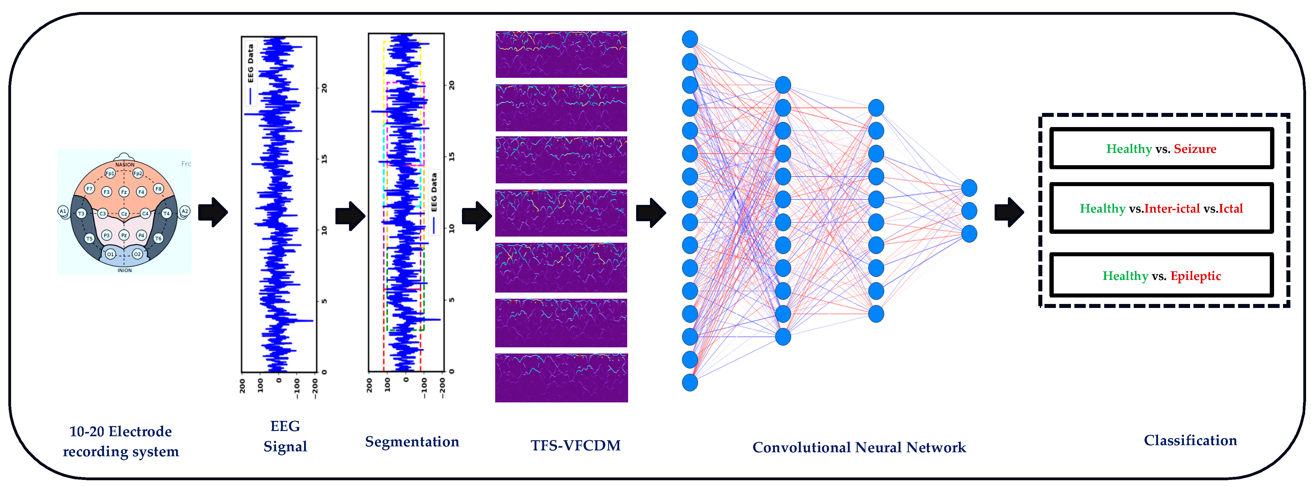
EEG-Based Seizure Detection Using Variable-Frequency Complex Demodulation and Convolutional Neural Networks

by
Yedukondala Rao Veeranki
,
Riley McNaboe
and
Hugo F. Posada-Quintero
*
Biomedical Engineering Department, University of Connecticut, Storrs, CT 06269, USA
*
Author to whom correspondence should be addressed.
Signals 2023, 4(4), 816-835; https://doi.org/10.3390/signals4040045
Submission received: 30 October 2023 / Revised: 21 November 2023 / Accepted: 25 November 2023 / Published: 28 November 2023
(This article belongs to the Special Issue Advanced Methods of Biomedical Signal Processing)

Abstract

:
Epilepsy is a complex neurological disorder characterized by recurrent and unpredictable seizures that affect millions of people around the world. Early and accurate epilepsy detection is critical for timely medical intervention and improved patient outcomes. Several methods and classifiers for automated epilepsy detection have been developed in previous research. However, the existing research landscape requires innovative approaches that can further improve the accuracy of diagnosing and managing patients. This study investigates the application of variable-frequency complex demodulation (VFCDM) and convolutional neural networks (CNN) to discriminate between healthy, interictal, and ictal states using electroencephalogram (EEG) data. For testing this approach, the EEG signals were collected from the publicly available Bonn dataset. A high-resolution time–frequency spectrum (TFS) of each EEG signal was obtained using the VFCDM. The TFS images were fed to the CNN classifier for the classification of the signals. The performance of CNN was evaluated using leave-one-subject-out cross-validation (LOSO CV). The TFS shows variations in its frequency for different states that correspond to variation in the neural activity. The LOSO CV approach yields a consistently high performance, ranging from 90% to 99% between different combinations of healthy and epilepsy states (interictal and ictal). The extensive LOSO CV validation approach ensures the reliability and robustness of the proposed method. As a result, the research contributes to advancing the field of epilepsy detection and brings us one step closer to developing practical, reliable, and efficient diagnostic tools for clinical applications.

1. Introduction

The World Health Organization (WHO) has found that epilepsy, a chronic noncommunicable group of neurological disorders of the brain, afflicts around 50 million people around the world regardless of age, race, and ethnicity [1,2,3]. In a normally functioning brain, small electrical impulses travel in a calculated and systematic manner, whereas epilepsy causes disruptions in the normal electrical balance, resulting in dynamic, repetitive seizures that can induce involuntary convulsions, loss of awareness, and altered sensations [4,5]. Patients are typically diagnosed with epilepsy after they have had two seizures that cannot be linked to any other previous/current medical condition [5]. The occurrence of seizures is not always synonymous with epilepsy and a comprehensive analysis must be administered to fully classify a patient as epileptic. To do so, healthcare providers will collect a full patient history and perform a neurological exam that includes the administration of an electroencephalogram (EEG), a diagnostic test that non-invasively measures the voltage potential resulting from current flow among the neurons of the brain [6,7]. In nominal brain activity, the electrical signals measured from EEG scalp electrodes follow a normal regulation. When a patient experiences a seizure, there is an increase in abnormal, large super-synchronous activity in either local or widespread areas with identifiable elliptic specific characteristics [8]. From EEG recordings, neurologists will visually scan the signals for any morphologic abnormalities representative of this activity that can indicate the presence of or even the type of epilepsy a patient may have to arrive at a final diagnosis.
While accuracy rates of epileptic diagnosis are high, traditional screening for epilepsy, most specifically the manual interpretation of EEG signals, has proven to be time-consuming when provided with many hours of recordings [9]. It has also shown to be variable and inaccurate in several cases, as the EEG readers level and technique of analysis may vary [10]. While this problem has been alleviated with the introduction of automatic seizure detection software, such implementations generally have poor sensitivity and are overfitted to a specific seizure occurrence, thus rendering them uncommon in most clinical settings. To avoid such issues and improve accuracy, new research has proposed various improvements and novel approaches to epileptic computer-aided diagnosis.
Recent research includes, but is not limited to, non-linear-, frequency-, time–frequency-, and time-based methods, as discussed by Acharya et al. [11]. Most of these methods have followed a similar approach, first establishing and extracting specific epileptic features in EEG waveforms, then performing a statistical analysis to rank the features, and finally, identifying the ideal classifier based on their respective performances. To further improve these methods, some groups have implemented deep convolution neural networks (CNN) to avoid feature extraction and selection [12,13,14,15]. This work has used custom CNNs and various DL models (Alexnet, VGG16, ResNet, etc.) in both 1D [12] and 2D [14,15] domains. The 2D approaches have explored the use of various inputs, including scaled spectrograms, the delta, and continuous wavelet transform scalograms.
In contrast to traditional machine learning algorithms, such as support vector machines or random forests, CNNs excel at automatically extracting hierarchical features from data, particularly in image-based tasks [16,17]. For EEG analysis, CNNs exhibit an inherent ability to differentiate subtle spatial and temporal relationships within time–frequency spectrum (TFS) images. This capability aligns well with the intricate variations in neural activity, characteristic of different epileptic states [18]. Furthermore, CNNs inherently possess translation invariance, allowing them to detect patterns regardless of their location within TFS images [18,19]. While other methods have demonstrated efficacy in various machine learning applications, the unique architecture and feature extraction capabilities of CNNs were deemed highly advantageous for deciphering the intricate patterns present in EEG data, ensuring a more nuanced and accurate classification of healthy and epilepsy states [20].
In this work, we propose using variable-frequency complex demodulation (VFCDM), a high-resolution, time–frequency domain method of analyzing various biomedical signals [21], to prepare 2D TFS of EEG signals for input into a deep convolution neural network for automated detection of epileptic traits. VFCDM can be summarized as a two-step procedure. First, complex demodulation is used to obtain an estimate of the time–frequency spectrum from which the dominant frequencies of interest are selected to be further refined. The second step involves passing the signal into a series of band-limited signals using a collection of low-pass filters (LPFs) to isolate the dominating frequencies. A Hilbert transform is applied to obtain an analytic signal for each band, providing a time–frequency spectrum containing simultaneous estimates of amplitude, frequency, and phase. To the best of our knowledge, no similar work has been performed with VFCDM spectrum-based inputs with convolutional neural networks.

2. Materials and Methods
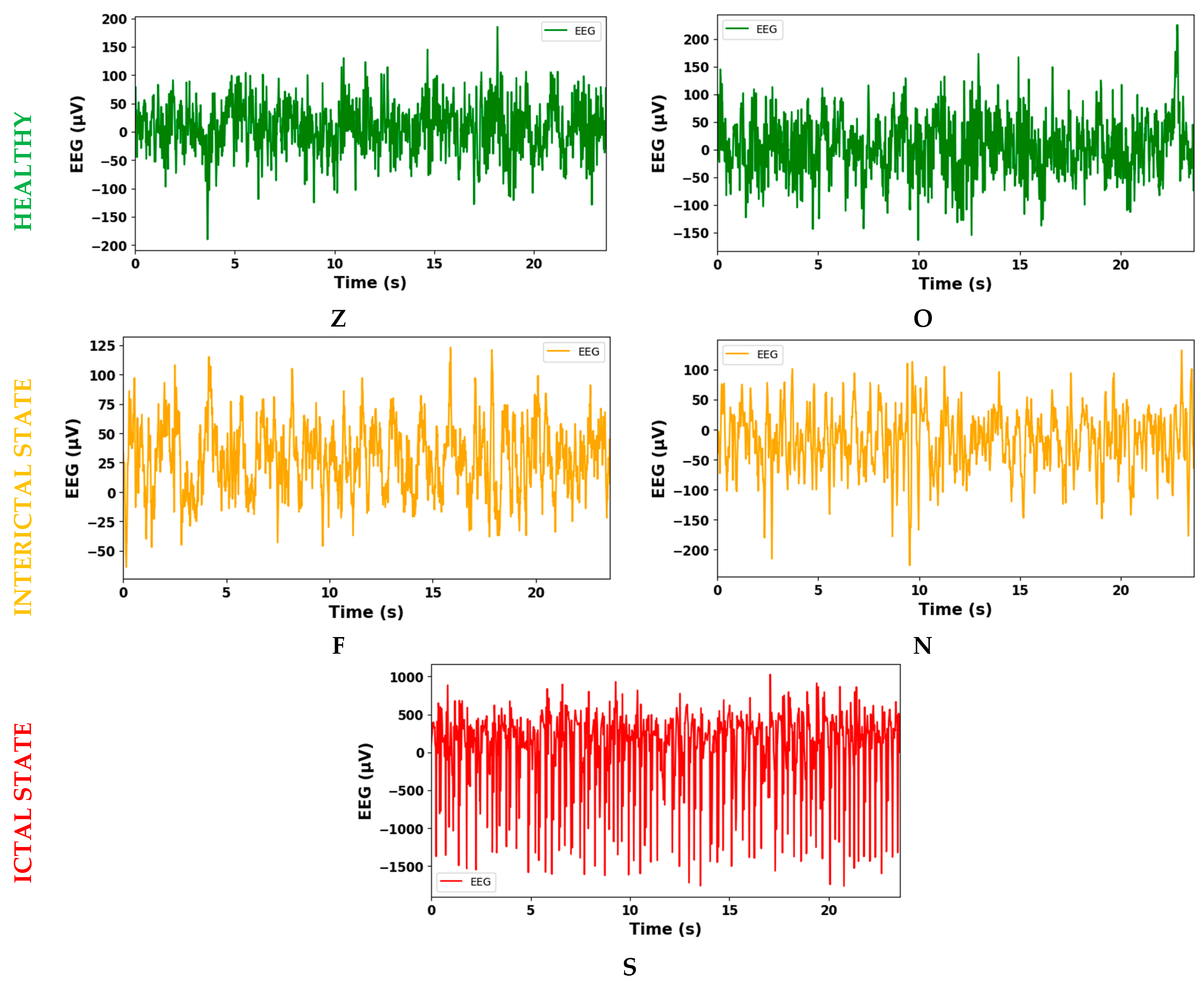
In this section, we present a detailed description of the basic steps involved during our research. We begin with an overview of the database used for EEG signal acquisition. This is followed by an explanation of the VFCDM method used for analysis and obtention of TFS. We then describe the CNN model that we used to accurately discriminate between different seizure states. Figure 1 illustrates the pipeline of the proposed methodology.

2.1. Database

In our study, we used the publicly available EEG dataset from the University of Bonn, as described by Andrzejak et al. [22]. The dataset has been extensively used to investigate various epilepsy states. It consists of five unique subsets (Z, O, N, F, and S) that are recorded using a 10–20 electrode placement system. Each subset contains one-channel 100 EEG segments of 23.6 s in length. The recordings were obtained at a sampling frequency of 173.61 Hz, resulting in 4097 samples for each EEG segment. Subsets Z and O were derived from recordings of five healthy volunteers, with Subset Z corresponding to segments collected with the eyes open and Subset O corresponding to segments collected with the eyes closed. N, F, and S subsets consist of EEG recordings taken from 5 epilepsy patients. Subsets N and F refer to seizure-free intervals during the interictal state. Note that Subset F includes segments recorded from the epileptogenic zone of the hippocampal formation, whereas Subset N signals were obtained from the contralateral hippocampal formation. Subset S includes EEG segments recorded during seizures (ictal state). Further, all the subsets were band-pass filtered to improve signal quality. The filter has a low cut-off frequency of 0.53 Hz and a high cut-off frequency of 40 Hz. To ensure the reliability of the dataset, an expert manually inspected all EEG segments for artifacts due to muscle activity and eye movements. The description of the dataset is shown in Table 1.
In this study, we used three distinct cases of grouping the segment into classes, designed to address specific classification scenarios. The details of these cases are presented in Table 2 for a comprehensive overview. Case I refers to the identification of segments collected from healthy subjects from seizure segments, whereas Case II refers to the three-class identification of healthy, interictal, and ictal segments. Finally, Case III refers to the identification of healthy vs. epileptic patients. Considering three classes in the classification scenarios enables the study to provide a comprehensive analysis of EEG data, allowing for the differentiation of healthy, interictal, and ictal states. This multi-class approach contributes to a deeper understanding of epilepsy and its neural dynamics, which is valuable for both diagnostic and research purposes.

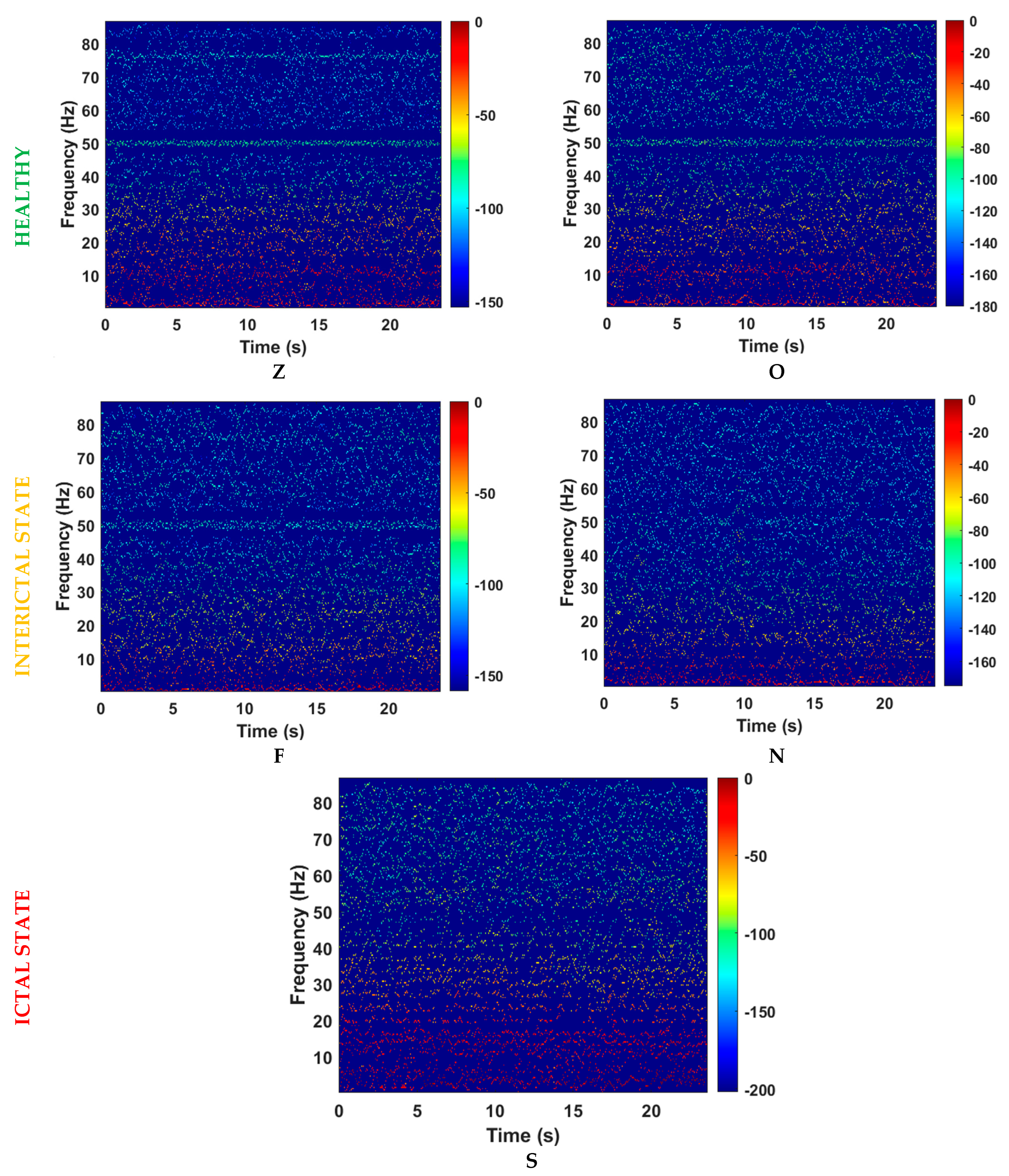
2.2. Variable-Frequency Complex Demodulation Algorithm

We used TFS obtained from EEG signals to objectively capture the changing dynamics in the central nervous system during normal and seizure conditions. To overcome the challenge of limited data samples, we employed a segmentation strategy that equally divided the EEG signals into seven segments. This increased the dataset and provided a more robust basis for TFS analysis. The foundation of our analysis is the use of the variable-frequency complex demodulation (VFCDM) technique. This approach has been extensively described in previous literature [21,23] and extensively validated with various physiological signals, such as blood pressure [21], renal blood flow [24], heart rate variability [25], and electrodermal activity [26,27].
The two-step process involved in estimating the TFS of EEG using VFCDM is as follows: First, an initial estimate of the TFS is obtained using fixed-frequency CDM (FFCDM) or complex demodulation. Second, the VFCDM approach is used to improve the time–frequency resolution by selecting the dominant frequencies of interest.

2.2.1. Complex Demodulation

In this step, each signal was decomposed into numerous band-limited signals using a series of low-pass filters (LPFs). Then, the Hilbert transform was applied to these signals. The result was analytical signals that provide estimates of instantaneous characteristics, such as amplitude, frequency, and phase, within their respective frequency bands. Consider a signal s t , which is characterized as a narrow-band oscillation. This signal exhibits a central angular frequency denoted as ω 1 and time-dependent attributes, including its instantaneous amplitude, represented as V t , and the initial phase, denoted as θ t . Additionally, s t includes a DC component, referred to as V d c , which contributes a constant offset to the signal:
s t = V d c + V t cos [ ω 1 t + θ t ]
The time-dependent attributes, such as V t , θ t for a specific carrier, can be extracted by multiplying s t by e j ω 2 t . This operation yields the unfiltered modulated signal m t :
m t = s t e j ω 2 t = V d c e j ω 2 t + V t 2 e j ω 1 ω 2 t + j θ t + e j ω 1 + ω 2 t j θ t
By assuming ω 1 ω 2 , the frequency spectrum of s t has been shifted left by an amount of ω 2 . If we subject s t to an LPF (cut-off frequency = ω c < ω 2 ), the signal m t is filtered such that only spectral components falling within the range [− ω c , ω c ] will remain. In this filtered output, the only component within this range corresponds to the difference frequency term. The outcomes can be expressed as follows:
m L P t = V t 2 e j θ t
V t = 2 m L P t
θ t = t a n 1 I m ( m L P t ) R e ( m L P t )
Here, m L P t is denoted as the CDM of a signal. The time derivative of θ t acts as a correction factor for the ω 2 , which can be employed to estimate the ω 1 of the input signal using Expression (6):
ω 1 t = ω 1 + d θ t d t

2.2.2. VFCDM

In a scenario where the modulating frequency is not constant, as previously described, but varies as a function of time, the signal s t can be represented in the following manner:
s t = V d c + V t cos 0 t 2 π f ( τ ) d τ + θ t ]
Following similar operations as those described in Equations (1) and (2), multiplying Equation (7) by e j 0 t 2 π f ( τ ) d τ results in the determination of both instantaneous amplitude V t and instantaneous phase θ t . This process yields:
m t = s t e j 0 t 2 π f ( τ ) d τ = V d c e j 0 t 2 π f ( τ ) d τ + V t 2 e j θ t + e j 0 t 4 π f τ d τ + θ t
Expanding from Equation (8), if we filter the signal m t using an ideal LPF, the result will be the filtered signal m L P t with identical instantaneous amplitude V t and phase θ t , as presented in Equations (4) and (5). The instantaneous frequency can be determined as provided in [28] and is given by:
f t = f 0 t + 1 2 π d θ ( t ) d t
In this study, the EEG signal is represented by the signal s(t). The Hilbert transform method was used to compute the instantaneous frequency and amplitude [29]. Applying the Hilbert transform to the equation above for all time points associated with the obtained low-pass-filtered frequency components resulted in the derivation of the complete time–frequency spectrum. The use of CDM and Hilbert transforms enabled the generation of a high-resolution TFS. This facilitated the accurate and precise extraction of amplitude information.
The procedure for implementing the TFS based on CDM is outlined as follows:
1.
Filter Design: Design a finite-impulse response LPF with a specified bandwidth ( F w ) and filter length ( N w ) . Set center frequencies as ( f 0 i ) :
f 0 i = 2 × F w i 1 ,   i = 1,2 , 3 , , i n t f m a x 2 × F w
  • 2 × F w = Spacing between neighboring center frequencies,
  • f m a x = Highest signal frequency.
2.
CDM Dominant Frequency Extraction: Employ the CDM technique to identify the dominant frequency within the defined bandwidth and iterate this process by incrementing  f 0 i  across the entire frequency band.
3.
Signal Decomposition: Decompose the signal into sinusoidal modulations using the CDM.
4.
Instantaneous Frequency Calculation: Calculate the instantaneous frequencies using Equation (9), based on the phase (as per Equation (5)) and the instantaneous amplitudes (as per Equation (4)) of each sinusoidal modulation component, using the Hilbert transform.
5.
Time–Frequency Representation: Obtain the TFR of the signal by using the estimated instantaneous frequencies and amplitudes, providing a detailed depiction of signal variations across both time and frequency domains. For more details about the VFCDM algorithm, please refer to [21].

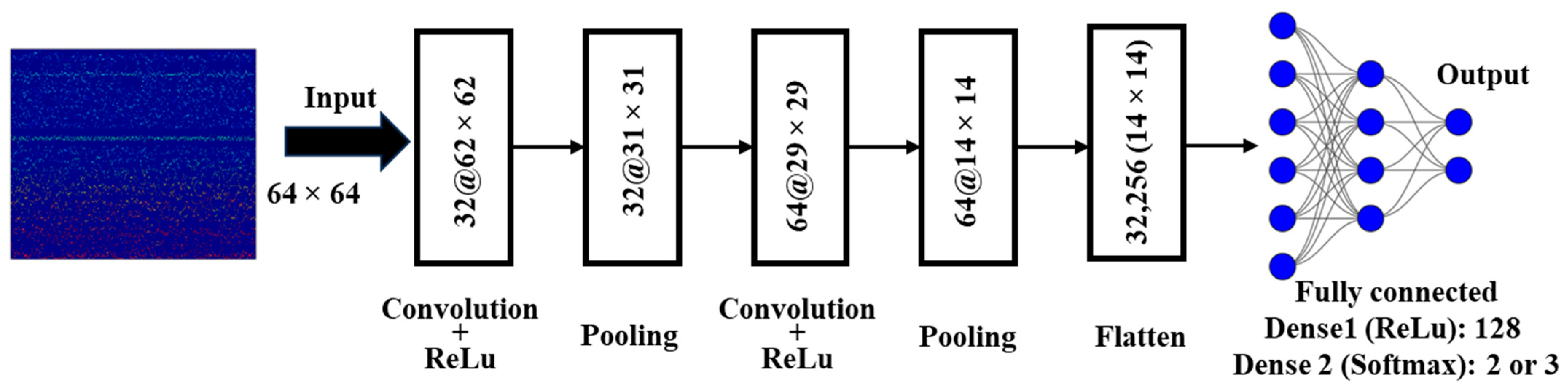
2.3. Convolutional Neural Networks

Convolutional neural networks are widely used across various domains due to their robust performance based on a deep feedforward architecture, reducing the number of parameters needed, smooth training, and expandability [30]. While there are specific CNN architectures that have been repeatedly used, all CNNs follow the same general structure that allows them to be easily modified, trained, and implemented depending on the desired application and restrictions presented [31,32]. CNNs have an intrinsic ability to automatically extract features and classify them, streamlining the typical extraction/classification work required in other models [33]. CNN operates by passing images through three sections that include an input layer, a collection of hidden layers, and an output layer. The hidden layers can be further segregated into specific components that consist of a (1) convolution layer, (2) pooling layer, and finally (3) a fully connected layer, which handles the classification.
(1)
Convolution Layer (CL)
The first hidden layer is the CL, which defines the operation of the entire CNN by extracting the features present based on the composition of its filters. The filter, commonly called a kernel or a weight vector, is a defined set of learnable parameters that is convoluted with a restricted area of the input that is dimensionally equivalent. This 2D convolution is repeated multiple times as the kernel slides along the length and width of the image. The frequency of the convolutions is controlled by the stride parameter, which defines the number of pixels the kernel shifts in each step. The output is then combined with an activation function that increases the non-linearity of the network. One of the most used functions is the rectified linear unit (ReLU), as it prevents the exponential growth in computational costs required to implement the CNN.
(2)
Pooling Layer (PL)
The next consecutive layer in the CNN is the PL, which works to reduce the size of feature maps and, in turn, reduce the overall computation time of the network. Since the location of a detected feature is not as relevant once identified [34], PLs, or rather sub/down-sampling layers, can reduce the parameters of the data by solely keeping meaningful information by implementing a specified pooling function (e.g., max, mean, and sum) determined by the type of PL. The function is applied using the sliding kernel method, similar to that of the CL. One of the most used pooling methods is max pooling.
(3)
Fully Connected Layer (FC)
The next consecutive layer is the FC layer. Defined by un-looped nodes, the FC is a feedforward layer that converts the condensed data layer into a 1D feature map. The map is calculated by taking the dot product of the weight matrix and input vector. A SoftMax function can also be commonly found in this layer.
The CNN used in this study consists of two CLs, two PLs, one flattened, and two FC layers. The CLs have the same architecture, both using a kernel of size 3 × 3 and stride 1. A ReLU activation function is implemented using the output. A max pooling layer of size 2 × 2 follows immediately after each CL to reduce the spatial dimension of the feature map. After the two sequential CL, the output is flattened, and two dense FC layers are used. The first FC layer consists of 128 ReLU-activated nodes and the second consists of 2 SoftMax-activated nodes. The structure is summarized in Figure 2.

2.4. Performance Evaluation of CNN

In order to thoroughly evaluate the performance of the model, a rigorous leave-one-subject-out (LOSO) cross-validation scheme was employed [35,36]. This meticulous approach ensured that the data from each patient were used for both the training and the testing of the model. Essentially, each patient served as an individual test case, with the remaining patients constituting training. This comprehensive evaluation strategy allowed us to assess the ability of the model to effectively generalize to the entire patient population. Additionally, the performance of the CNN was evaluated using accuracy (Acc), precision (Pre), recall (Rec), and F1-score (F1) metrics [37]. The mathematical expressions used to calculate each metric are described in Table 3.

3. Results

The representative EEG signals in healthy, interictal, and ictal states are shown in Figure 3. The amplitude and fluctuation characteristics of the representative EEG in each state are described below.
Z and O—Healthy State: In this state, the EEG signals have a root mean square (RMS) amplitude that is typically in the range of 40 to 43 µV. This low amplitude, with amplitude fluctuations averaging 28 to 29 µV, indicates a consistent and stable level of neural activity. These patterns are indicative of a baseline of neuronal excitability. This means that neuronal activities in the healthy brain remain within a steady and balanced range, typically hovering around 40–43 µV.
F and N—Interictal State: RMS amplitude values are significantly higher, ranging from 49 to 50.5 µV, in this state. This increased RMS amplitude may indicate increased neuronal excitability compared to healthy states. Examining fluctuations, interictal states show more pronounced and erratic fluctuations, reaching 49 to 50.5 µV. These increased fluctuations are indicative of neuronal instability, often associated with epilepsy or pre-seizure conditions. The increased variability reflects a transition to an altered neural state that may be predisposing the brain to seizure activity.
S—Ictal State: This state has an intermediate range of RMS amplitude values, around 36.5 µV. This is significantly lower than the interictal states. This suggests a neural state in transition, as these values fall between the amplitudes of the healthy and interictal states. However, the most characteristic feature of ictal states is the presence of intense amplitude fluctuations. These can reach up to 478.5 µV. These fluctuations are significantly more pronounced than those observed in healthy or interictal states and indicate an ongoing epileptic event.
These EEG signal characteristics and differences provide valuable insights into the state of the brain. Healthy states are characterized by stable and low-amplitude signals, interictal states show heightened fluctuations, and ictal states demonstrate rapid and synchronous neuronal activity. These distinctions are crucial for diagnosing and monitoring epilepsy and understanding the underlying neural dynamics.
The TFS of the representative EEG signals in healthy, interictal, and ictal states are shown in Figure 4. To find the variations across these states, we conducted a comprehensive analysis of several key features within each TFS. Specifically, we examined the mean, maximum, standard deviation, spectral energy, dominant frequency, and % of significant frequency transitions. This analysis provides valuable insights into the distinctions between healthy, interictal, and ictal states.
Z and O—Healthy State: These states exhibit moderate neural activity, as evidenced by the mean frequency range around 14.47 Hz. Their highest spectral power is within the range of 804 dB, indicating that extreme spikes in activity are relatively infrequent. The stability of neural dynamics is observed in the mean of the standard deviation of TFR, which remains around 65.6 Hz. The mean of total power suggests that there is a substantial amount of spectral power in these signals, at approximately 5.9241 × 10⁴ dB. Both Z and O have a peak frequency around 3 Hz, indicating the frequency with the maximum power. The mean of dominant frequency for healthy states is about 5.4 Hz, which is relatively low. These states also exhibit 28% of significant frequency transitions, implying a moderate variability in neural dynamics.
F and N—Interictal State: These states show a lower level of neural activity, as indicated by a mean frequency range of around 10 Hz. Their highest spectral power is within the range of 550 dB, lower than in the healthy state. The stability of neural dynamics remains moderate, at approximately 42 Hz. The mean of total power in the interictal state is about 4.1827 × 10⁴ dB, indicating less spectral power. Surprisingly, the peak frequency for interictal states reaches 500 Hz, suggesting a shift toward higher frequencies. A distinctive feature of the interictal state is the mean of dominant frequency, which is approximately 97 Hz, indicating increased activity in higher frequency bands. These states also have a moderate 5% of significant frequency transitions.
S—Ictal State: The ictal state stands apart with notably distinct TFS characteristics. This state is marked by a substantially higher mean frequency range, at approximately 1.6776 × 10³ Hz, pointing to intense neural activity during seizures. The mean of maximum TFS reaches around 6.3788 × 10⁴ dB, signifying high levels of neural activity during ictal events. However, this heightened activity also results in a significantly elevated stability of TFS. In terms of mean total power, the state exhibits notably high values, reaching approximately 6.8699 × 10⁶ dB, indicating a substantial amount of spectral power in these signals. Unlike healthy and interictal states, the ictal state exhibits a peak frequency close to 0 Hz, which suggests a wide range of frequency activity during seizures. The mean dominant frequency is remarkably low, approximately 0.0072 Hz, underlining the diversity of neural dynamics during seizures. In contrast to the other states, ictal states have a low significant frequency transition, around 0.0244%, suggesting relatively stable frequency patterns during seizures.
The TFS image of each EEG segment was used as input to the CNN for classifying various combinations of healthy and epileptic states. The results of each case are described below.

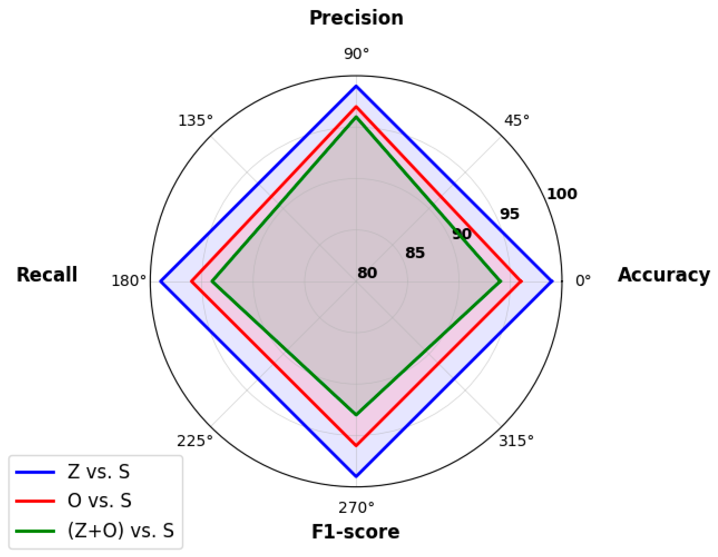
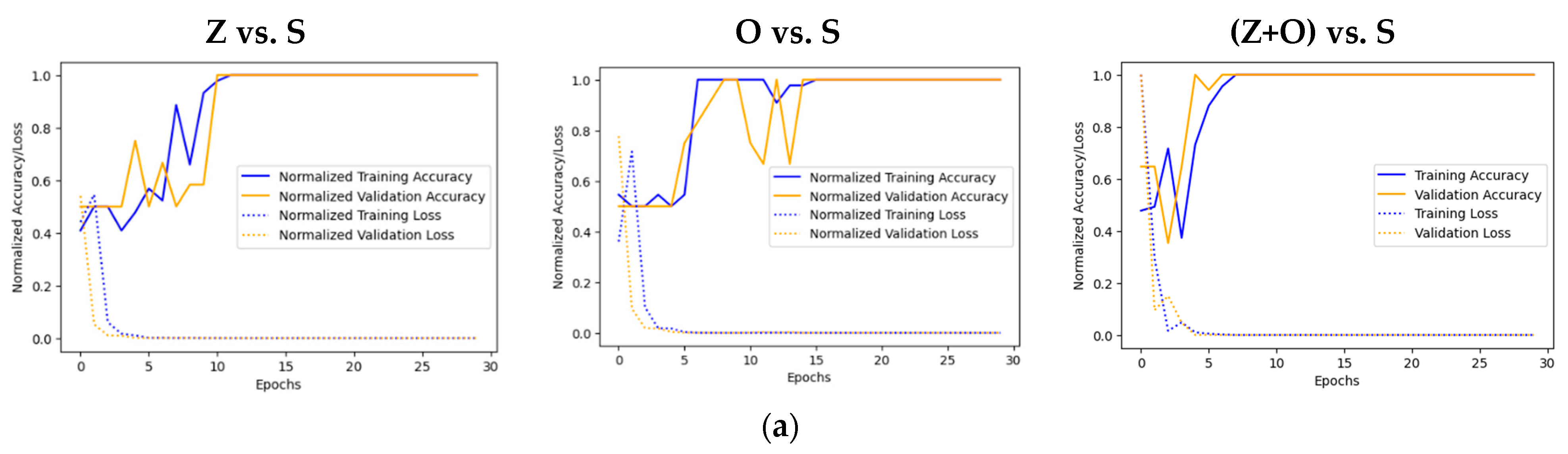
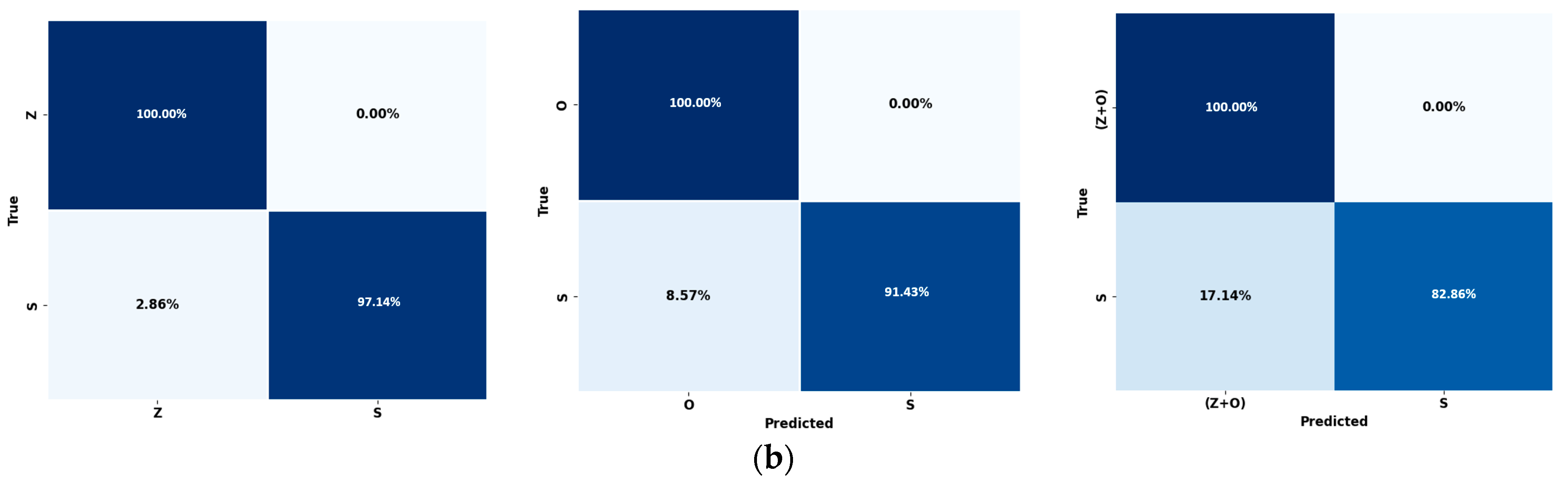
3.1. Case I: Healthy vs. Ictal State

The performance of CNN in classifying healthy and ictal states using LOSO CV is shown in Figure 5. The results demonstrate the robustness of the CNN model across multiple state classifications. The model yielded the highest Acc, Pre, Rec, and F1 of 99% when classifying healthy state Z compared to ictal state S. Additionally, the model achieved 96% accuracy in differentiating healthy O from ictal S, with Pre and Rec of 97% and 96%, respectively. The model also achieved 94% accuracy when considering the combined healthy states (Z+O) versus the ictal state S. The precision rate remains high at 96%, and the recall rate of 94% demonstrates the ability of the model to capture the majority of (Z+O) instances. These results demonstrate the ability of the CNN model to accurately characterize different states based on TFS images.
The training and validation metrics of the CNN, as shown in Figure 6a, exhibit different patterns in different classification scenarios. In the Z vs. S scenario, both normalized training accuracy (NTA) and normalized validation accuracy (NVA) fluctuated until the 10th epoch, but then stabilized at 1.0. The normalized training loss (NTL) and normalized validation loss (NVL) consistently decreased to 0, indicating a stable learning process. For O vs. S, NTA started at 0.54, reaching 1.0 by the 7th epoch, with NTL declining from 0.36 to 0. NVA steadily increased to 1.0, and NVL consistently decreased to 0, with minor fluctuations from the 10th to the 15th epoch. In (Z+O) vs. (S), the model exhibited significant stability, with NTA reaching 1.0 by the 7th epoch, NTL decreasing to 0, and NVA increasing to 1.0. This highlights the model’s consistent performance across various classification scenarios.
Figure 6b shows the normalized confusion matrices of the CNN for different classification scenarios. For Z vs. S binary classification, the model yielded 100% true positives (TP) and true negatives (TN), while avoiding false positives (FP) and false negatives (FN). In the O vs. S case, the model demonstrated strong performance, achieving a 100% TN rate while accurately detecting ictal states. However, there were some instances where ictal states were misclassified as healthy states, leading to an 8.57% FN rate. Finally, in the (Z+O) vs. S classification, the model accurately identified S with a TP rate of 2.86%. Nonetheless, the model exhibited an FP rate of 17.14%, indicating the misclassification of Z+O as S state. Despite this, the model demonstrated high overall Acc and F1. Collectively, the results highlight the model’s ability to effectively distinguish between these different states.

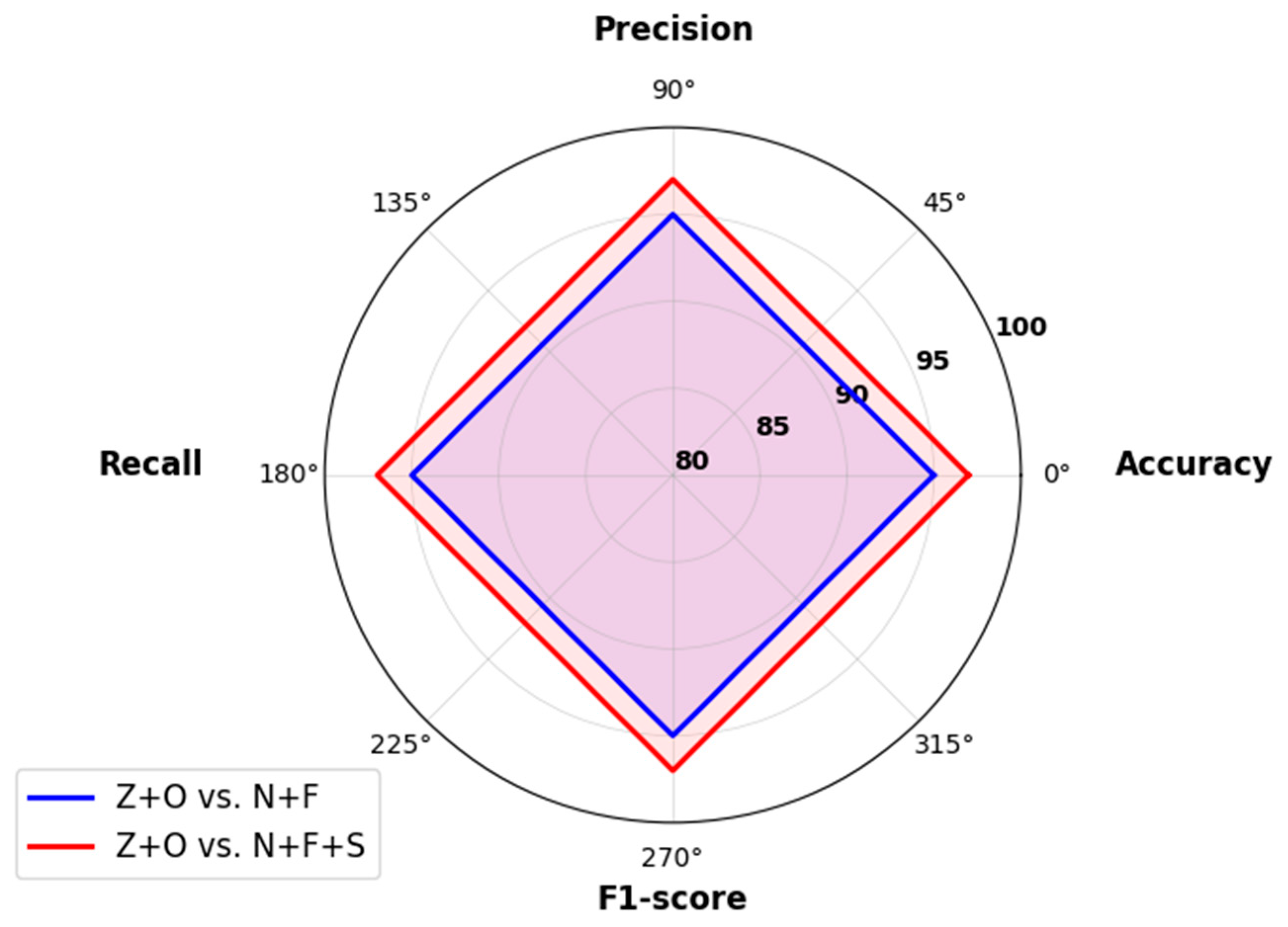
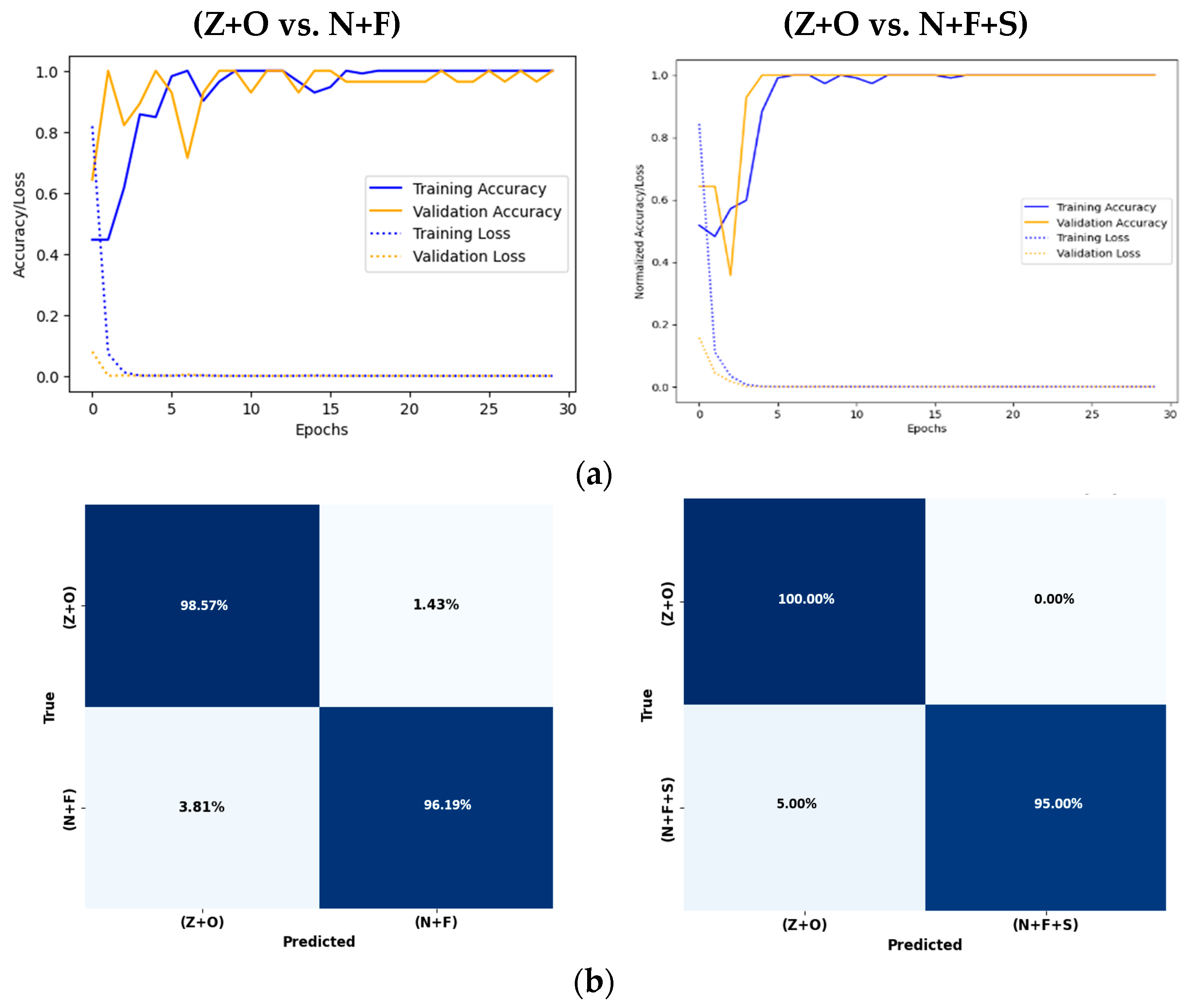
3.2. Case II: Healthy vs. Epilepsy Subjects

In our investigation, to classify healthy and epilepsy subjects using CNN, we considered two different scenarios. Specifically, we evaluated the effectiveness of the CNN in classifying various combinations of healthy (Z and O) and epilepsy (N, F, and S) states. The performance metrics for each case are shown in Figure 7. In the first case, when distinguishing between a collective group of healthy subjects (Z and O) and interictal subjects (N and F), the model achieved an Acc of 95%. Pre and Rec metrics, both at 95%, indicate the model accuracy while balancing false positives and negatives. This balance is further evidenced by its F1 of 95%. In the second case, we aimed to classify the combined healthy subjects (Z and O) from the interictal (N and F) and ictal (S) states of epileptic subjects. The model achieved 97% Acc, indicating a high degree of overall correctness. Further, Pre and Rec metrics were also 97%, indicating the model’s ability to accurately identify relevant data while managing false alarms.
The CNN training and validation metric curves shown in Figure 8a for healthy vs. epileptic subjects demonstrate effective learning. For the (Z+O) vs. (N+F+S) scenario, the model showed continuous improvement, reaching an NTA of 1.0 and an NTL of 0.0 by the 7th epoch. Although the NVA curve showed fluctuations, it also showed growth. Similarly, in (Z+O) vs. S, the model maintained stability during its learning process, with the NTA reaching 1.0 by the 6th epoch and the NTL decreasing to 0.0. The NVA continued to grow and remained stable. These results emphasize the model’s effectiveness in accurately classifying the chosen state combinations.
The normalized confusion matrices for the two significant classification scenarios considered in the CNN model are shown in Figure 8b. The model accurately classified Z+O from N+F combinations. It had a TPR of 98.57% for the identification of N+F states, with a low FNR of 1.43%. The TNR was 96.19% and the FPR was effectively minimized to 3.81%. In the complex classification scenario Z+O vs. N+F+S, the model demonstrated robust performance, yielding 100% TNR to accurately identify N+F+S states and maintaining a 5% FPR. This indicates minimal errors in the classification of (Z+O) as (N+F+S). These results demonstrate the model’s proficiency in the classification scenarios with remarkable overall Acc and F1 values.

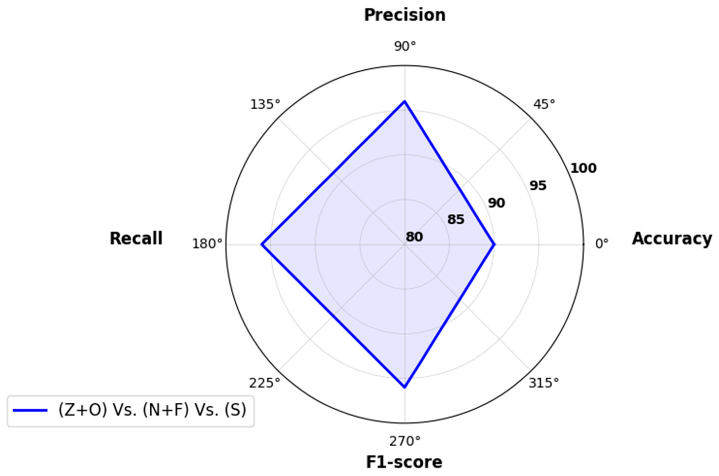
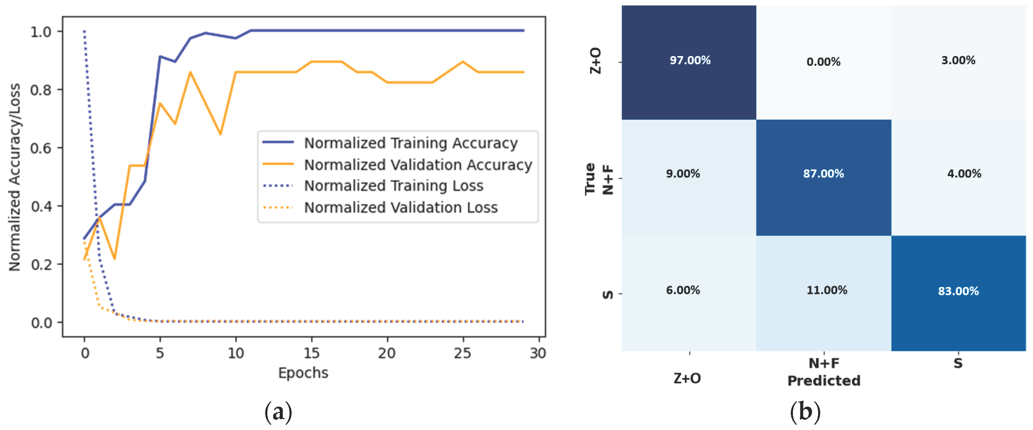
3.3. Case III: Healthy vs. Interictal vs. Ictal States

In this case, we extended our analysis to a more intricate scenario of distinguishing between healthy states (Z and O), interictal states (N and F), and ictal states (S), separately. The CNN performance metrics for this case are shown in Figure 9. In this comprehensive case, the CNN model yielded an Acc of 90%. Furthermore, the precision, recall, and F1-score metrics all reached an impressive 96%. These metrics emphasize the model’s ability to make accurate predictions. The model also demonstrated an effective approach to managing false positives and false negatives, maintaining a harmonious balance.
The CNN’s training and validation metric curves, as depicted in Figure 10a, provide a visual representation of the model’s performance in the scenario of (Z+O) vs. (N+F) vs. S. In this specific case, we observed a unique pattern compared to previous scenarios. The learning curves for both NTA and NVA exhibited fluctuations, with NTA reaching 1.0 by the 12th epoch and NVA at 0.85 by the 27th epoch. On the other hand, NTL and NVL consistently decreased, highlighting the ability of the model to determine complex differences within these state combinations. The fluctuating patterns reflect the adaptability of the model even in scenarios where accuracy and loss metrics occasionally vary.
In the multi-class classification scenario with Z+O, N+F, and S, as shown in Figure 10b, the CNN model exhibited significant performance. It yielded a 97% TPR for accurately categorizing Z+O, demonstrating a high degree of accuracy in classifying this state. Notably, Z+O was rarely misclassified as other states, as indicated by the absence of FPs. The model also demonstrated an 87% TPR for N+F, with a 9% FNR, suggesting reasonable identification of N+F. However, N+F had a 4% FPR, indicating rare misclassification as S. For the ictal state, the model achieved a significant 83% TPR, accompanied by a 6% FNR. Additionally, there was an 11% FPR for S, signifying few misclassifications as other states. Overall, the model showcased its capability to differentiate between these states, maintaining a good balance of accuracy and false positive/negative rates in this complex multi-class classification scenario.

4. Discussion

The accurate and timely detection of epileptic seizures remains a critical challenge in clinical neurology. While scalp EEG has long been the gold standard for seizure monitoring, manual interpretation of EEG data is both time-consuming and prone to human error. Automated seizure detection systems that can provide real-time alerts have the potential to significantly improve patient care by enabling timely interventions and reducing the risk of seizure-related complications. They also have the potential to reduce the burden on healthcare professionals and enhance the overall management of epilepsy. This study investigated the application of VFCDM and CNN approaches in epilepsy detection using EEG signals. The focus was on exploring the possibility of developing an automated system for differentiating healthy, interictal, and ictal states. The VFCDM time–frequency spectrum that accounts for non-linear and non-stationary variations of EEG signals was used to develop the system. The results of the proposed method showcased high accuracy and the ability to manage both simple and complex classification scenarios.
In this study, the Bonn dataset was specifically selected due to its robustness and extensive use in epilepsy research. Its publicly available nature promotes reproducibility and facilitates comparisons with previous studies. The dataset includes subsets representing healthy, interictal, and ictal states. It provides intricate neural activity patterns, making it well suited for multi-class classification tasks. To ensure the integrity and high quality of the data, rigorous preprocessing steps, including band-pass filtering and artifact removal, were implemented. The partitioning of the dataset into training and validation sets was carried out with the utmost care and consideration, using stratification techniques to ensure unbiased training and evaluation of the models. These deliberate choices profoundly influenced the results of the study, yielding valuable insights into the dynamics of epilepsy and significantly impacting the efficacy of learning-based methods.
EEG signals exhibit distinct characteristics that differentiate between healthy and epilepsy states. In healthy individuals, EEG signals show low amplitude and stable neural activity, reflecting a consistent and balanced level of neuronal excitability. In contrast, interictal states, which are the EEG patterns observed between seizures, show increased amplitude and pronounced fluctuations, suggesting greater neuronal instability, often associated with epilepsy or pre-seizure conditions. Ictal states, the EEG patterns observed during seizures, exhibit an intermediate range of amplitude values but are characterized by intense amplitude fluctuations. These distinct EEG signal characteristics form the basis for effective seizure detection and classification.
The analysis of the TFS of EEG signals using VFCDM further emphasized these distinctions. Healthy states demonstrated moderate neural activity with a mean frequency range of around 14.47 Hz. These states also exhibited stable dynamics. Interictal states exhibited lower neural activity with a mean frequency range of around 10 Hz. A significant shift toward higher frequencies was also observed in these states. Ictal states yielded substantially higher mean frequency ranges and intense neural activity. This demonstrates that there is a wide range of frequency activity during seizures. These TFS characteristics align with the amplitude and fluctuation patterns observed in EEG signals.
The CNN model exhibited significant classification performance. The model consistently demonstrated high performance for all three cases considered in the study. It accurately classified both simple and complex combinations of states while maintaining a balance between true positives and negatives. The highest performance (99%) was achieved when classifying healthy (Z) and seizure states. The model adapted well to complex differences within these state combinations, thus effectively managing variations in Acc and loss metrics.
Previous studies have reported various methods for automated epilepsy detection using the Bonn dataset. Numerous studies have addressed epilepsy detection, employing diverse methodologies and classifiers. Table 4 provides a comparison of our proposed work with the state-of-the-art methods. Faust et al. (2010) [38] employed the Yule–Walker method and an SVM, yielding an Acc of 93.3%. Similarly, Acharya et al. (2009) [39] computed non-linear measures, such as correlation and fractal dimension, and the Hurst and Lyapunov exponent. These features were fed into the GMM classifier and achieved an accuracy of 96.1%. These findings emphasize the potential of advanced methods and classifiers for precise epilepsy diagnosis. Researchers such as Acharya et al. (2013) [40] have focused on signal-processing methods. They employed DWT frequency band features and SVM for epilepsy detection, maintaining a high accuracy of 96.0%. Additionally, Sharmila et al. (2018) [41] used DWT entropy features with an SVM classifier, highlighting the significance of exploring various signal-processing techniques for improved classification.
The emergence of deep learning approaches in the field of EEG analysis is evident in the studies by Acharya et al. (2018) [13] and Ilias et al. (2023) [14]. While Acharya et al. [13] achieved an accuracy of 88.7% using 1D EEG features and a CNN, Ilias et al. [14] adopted spectrogram analysis with a CNN to attain an accuracy of 97.0%. These studies showcase the potential of deep learning models in EEG analysis and the advantages they offer in terms of accuracy. Further, the introduction of innovative feature extraction methods has significantly influenced epilepsy detection. Mahfuz et al. (2021) [15] employed CWT with a CNN classifier, achieving an accuracy of 98.46%. Their research highlights the potential of wavelet-based features when coupled with CNN models. Additionally, Yuan et al. (2017) [42] applied CWT scalogram analysis with GPCA and SDAE, achieving absolute accuracy and precision. These studies illustrate the ability of advanced feature extraction techniques.
Some studies have also used neural network architectures. Hussein et al. (2019) [43] introduced TD features and RNN/LSTM for epilepsy detection, achieving an accuracy of 100%. Meanwhile, Chanu et al. (2023) [44] used DWT with SONN, resulting in an accuracy of 99.2%. These studies emphasized the potential of neural networks in EEG analysis. Recent advancements in deep learning are reflected in studies such as that of Islam et al. (2022) [45], who explored TD features with the Epileptic-Net model, achieving an accuracy ranging from 99.95% to 99.98%. Further, Bhattacharyya et al. (2017) [46] examined EWT features with RF, reaching an accuracy of 99.4%. This highlights the need for a multimodal approach to enhance diagnostic accuracy.
Additionally, Sharma et al. (2017) [47] employed flexible WT and fractal dimension with SVM, achieving an accuracy of 99.2%. Their research shows the potential of combining multiple techniques for enhanced results. Further, Goel et al. (2023) [48] introduced recurrence plots with an SVM classifier, achieving an accuracy of 98.21% and a precision rate of 99.61%. These studies showcase the potential of unique approaches in feature extraction and classification.
Table 4. Comparison of various studies related to the automatic detection of epileptic classes using the Bonn University database of EEG signals.
AuthorMethodClassifierCross-ValidationPerformance (%)
AccPreRecF1
Faust et al. 2010 [38]Yule–WalkerSVM $˗93.3˗˗˗
Acharya et al. 2009 [39]Non-linear measuresGMM $˗96.1˗˗˗
Acharya et al. 2013 [40]DWT Frequency BandsSVM $˗96.0˗˗˗
Sharma et al. 2017 [47]Flexible WT/Fractal DimensionSVM10-Fold99.2˗˗˗
Acharya et al. 2018 [13]1D EEG FeaturesCNN10-Fold88.7˗˗˗
Ilias et al. 2023 [14]Spectrogram/DeltaCNN10-Fold97.097.14–97.18 *96.00–97.99 *96.41–97.52 *
Mahfuz et al. 2021 [15]CWTCNNSplit 10/9098.46˗˗˗
Hussein et al. 2019 [43]TDRNN/LSTM3/5/10-Fold100˗˗˗
Chanu et al. 2023 [44]DWTSONNSplit 30/7099.29810098.99
Islam et al. 2022 [45]TDEpileptic-Net10-Fold99.95–99.98 *˗˗˗
Yuan et al. 2017 [42]CWT ScalogramGPCA/SDAESplit 80/20100100100100
Ullah et al. 2018 [12]TDP-1D-CNN10-Fold97.4–100 *˗˗˗
Guo et al. 2011 [49]Genetic ProgrammingKNNSplit 60/4093.5˗˗˗
Bhattacharyya et al. 2017 [46]EWTRF10-Fold99.4˗˗˗
Sharmila et al. 2018 [41]DWT EntropySVMSplit 50/5078–100 *˗˗˗
Goel et al. 2023 [48]Recurrence PlotsSVM-98.2199.61˗˗
Abdulhay et al. 2020 [50]Entropy, non-linear, and spectraSCANN10-Fold98.5˗˗˗
Proposed ApproachVFCDMCNNLOSO CV90–99 *96–99 *94–99 *93–99 *
SVM = support vector machine; GMM = Gaussian mixture model; RF = random forest; RNN = recurrent neural network; LSTM = long short-term memory; SONN = self-organizing neural network; GPCA = global principal component analysis; SDAE = stacked denoising autoencoders; P-1D-CNN = pyramidal-1d CNN; WT = wavelet transform; DWT = discrete WT; EWT = empirical WT; CWT = continuous WT; TD = time domain. $ Performance of the classifier is evaluated using receiver operating characteristic (ROC) analysis. * Performance range in classifying between various combinations of healthy and epileptic states.
Building upon the foundations laid by previous works, the proposed approach in this study, which used VFCDM and CNN for automated epilepsy detection, demonstrated promising performance, with accuracy ranging from 90% to 99% across various classification scenarios. This performance compares favorably with other state-of-the-art techniques, such as those based on SVMs or RNNs, which typically achieve accuracies in the range of 80% to 95%. Interestingly, to the best of our knowledge, there are very few LOSO CV studies. LOSO CV offers a more robust evaluation of biomedical applications by accounting for subject-specific variability and ensuring clinical relevance.
In addition to its performance, the proposed approach offers several advantages over other techniques. VFCDM stands out from other TF methods in its ability to effectively handle the non-linear and non-stationary characteristics of EEG signals. By using variable frequencies, VFCDM adapts to the changing nature of EEG data, capturing intricate dynamics and preserving instantaneous amplitudes, crucial for identifying and characterizing neural activity. VFCDM’s non-parametric nature allows it to handle complex and unpredictable EEG patterns without relying on a priori assumptions, making it a powerful tool for analyzing EEG signals. Additionally, CNNs are powerful classifiers that can learn complex patterns from these features, making them well suited for seizure detection.
While the VFCDM and CNN combination demonstrated promising potential for automated epilepsy detection, further research is needed to fully evaluate its clinical utility. Additional studies on larger, more diverse datasets are required to confirm the approach’s generalizability. Prospective clinical trials should also be conducted to assess its effectiveness in real-world settings. Additionally, addressing limitations, such as the limited dataset scope, exclusion of the pre-ictal state, focus on single-channel EEG analysis, lack of testing in noisy environments, and the absence of comprehensive comparisons with other methods, will strengthen the proposed approach’s clinical applicability.
In summary, the proposed approach represents a promising step forward in the development of automated seizure detection systems. The combination of VFCDM and CNN offers a powerful and efficient method for extracting and classifying non-linear features from EEG signals. This approach has the potential to significantly improve patient care by reducing the burden on healthcare professionals and enhancing the overall management of epilepsy.

5. Conclusions

This study presented a novel approach for automated epilepsy detection using VFCDM in combination with CNN. The results demonstrated that VFCDM effectively extracted non-stationary and non-linear variations in EEG signals, enabling the discrimination of various epileptic states. The application of this method, in combination with LOSO CV, demonstrated significant performance, ranging from 90% to 99%. Considerations for real-world clinical implementation, including the development of user-friendly tools and validation in clinical settings, are vital for the practical application of this methodology.

Author Contributions

Y.R.V., formal analysis, investigation, methodology, resources, software, validation, visualization, writing—original draft preparation; R.M., methodology, writing—original draft preparation, validation, visualization; H.F.P.-Q., conceptualization, supervision, formal analysis, investigation, methodology, validation, visualization, writing—review and editing. All authors have read and agreed to the published version of the manuscript.

Funding

This research received no external funding.

Institutional Review Board Statement

As the data were pre-existing and publicly accessible, ethical review and approval were not necessary for this study.

Data Availability Statement

The dataset was retrieved from: https://repositori.upf.edu/handle/10230/42894 (accessed on 1 September 2023).

Acknowledgments

In this study, we used the EEG signals that are publicly made available by Bonn University. We acknowledge the contributions of the dataset creators, Andrzejak et al., for making this valuable resource publicly available. The dataset was retrieved from: https://repositori.upf.edu/handle/10230/42894 (accessed on 1 September 2023), and played a crucial role in the success of our research.

Conflicts of Interest

The authors declare no conflict of interest.

References

  1. Epilepsy. Available online: https://www.who.int/news-room/fact-sheets/detail/epilepsy (accessed on 16 October 2023).
  2. England, M.J.; Liverman, C.T.; Schultz, A.M.; Strawbridge, L.M. Epilepsy across the Spectrum: Promoting Health and Understanding.: A Summary of the Institute of Medicine Report. Epilepsy Behav. 2012, 25, 266–276. [Google Scholar] [CrossRef] [PubMed]
  3. Abreu, M.; Carmo, A.S.; Franco, A.; Parreira, S.; Vidal, B.; Costa, M.; Peralta, A.R.; da Silva, H.P.; Bentes, C.; Fred, A. Mobile Applications for Epilepsy: Where Are We? Where Should We Go? A Systematic Review. Signals 2022, 3, 40–65. [Google Scholar] [CrossRef]
  4. Epilepsy and Seizures. Available online: https://www.ninds.nih.gov/health-information/disorders/epilepsy-and-seizures (accessed on 16 October 2023).
  5. Epilepsy—Seizure Types, Symptoms and Treatment Options. Available online: https://www.aans.org/ (accessed on 16 October 2023).
  6. Biasiucci, A.; Franceschiello, B.; Murray, M.M. Electroencephalography. Curr. Biol. 2019, 29, R80–R85. [Google Scholar] [CrossRef] [PubMed]
  7. Noachtar, S.; Rémi, J. The Role of EEG in Epilepsy: A Critical Review. Epilepsy Behav. 2009, 15, 22–33. [Google Scholar] [CrossRef]
  8. Ramakrishnan, S.; Rayi, A. EEG Localization Related Epilepsies. In StatPearls; StatPearls Publishing: Treasure Island, FL, USA, 2023. [Google Scholar]
  9. Nigam, V.P.; Graupe, D. A Neural-Network-Based Detection of Epilepsy. Neurol. Res. 2004, 26, 55–60. [Google Scholar] [CrossRef] [PubMed]
  10. Angus-Leppan, H. Diagnosing Epilepsy in Neurology Clinics: A Prospective Study. Seizure 2008, 17, 431–436. [Google Scholar] [CrossRef]
  11. Acharya, U.R.; Vinitha Sree, S.; Swapna, G.; Martis, R.J.; Suri, J.S. Automated EEG Analysis of Epilepsy: A Review. Knowl.-Based Syst. 2013, 45, 147–165. [Google Scholar] [CrossRef]
  12. Ullah, I.; Hussain, M.; Qazi, E.-H.; Aboalsamh, H. An Automated System for Epilepsy Detection Using EEG Brain Signals Based on Deep Learning Approach. Expert Syst. Appl. 2018, 107, 61–71. [Google Scholar] [CrossRef]
  13. Acharya, U.R.; Oh, S.L.; Hagiwara, Y.; Tan, J.H.; Adeli, H. Deep Convolutional Neural Network for the Automated Detection and Diagnosis of Seizure Using EEG Signals. Comput. Biol. Med. 2018, 100, 270–278. [Google Scholar] [CrossRef]
  14. Ilias, L.; Askounis, D.; Psarras, J. Multimodal Detection of Epilepsy with Deep Neural Networks. Expert Syst. Appl. 2023, 213, 119010. [Google Scholar] [CrossRef]
  15. Rashed-Al-Mahfuz, M.; Moni, M.A.; Uddin, S.; Alyami, S.A.; Summers, M.A.; Eapen, V. A Deep Convolutional Neural Network Method to Detect Seizures and Characteristic Frequencies Using Epileptic Electroencephalogram (EEG) Data. IEEE J. Transl. Eng. Health Med. 2021, 9, 2000112. [Google Scholar] [CrossRef]
  16. Yamashita, R.; Nishio, M.; Do, R.K.G.; Togashi, K. Convolutional Neural Networks: An Overview and Application in Radiology. Insights Imaging 2018, 9, 611–629. [Google Scholar] [CrossRef] [PubMed]
  17. Ganapathy, N.; Veeranki, Y.R.; Swaminathan, R. Convolutional Neural Network Based Emotion Classification Using Electrodermal Activity Signals and Time-Frequency Features. Expert Syst. Appl. 2020, 159, 113571. [Google Scholar] [CrossRef]
  18. Craik, A.; He, Y.; Contreras-Vidal, J.L. Deep Learning for Electroencephalogram (EEG) Classification Tasks: A Review. J. Neural Eng. 2019, 16, 031001. [Google Scholar] [CrossRef]
  19. Jacovi, A.; Shalom, O.S.; Goldberg, Y. Understanding Convolutional Neural Networks for Text Classification. arXiv 2020, arXiv:1809.08037. [Google Scholar]
  20. Tajbakhsh, N.; Shin, J.Y.; Gurudu, S.R.; Hurst, R.T.; Kendall, C.B.; Gotway, M.B.; Liang, J. Convolutional Neural Networks for Medical Image Analysis: Full Training or Fine Tuning? IEEE Trans. Med. Imaging 2016, 35, 1299–1312. [Google Scholar] [CrossRef]
  21. Wang, H.; Siu, K.; Ju, K.; Chon, K.H. A High Resolution Approach to Estimating Time-Frequency Spectra and Their Amplitudes. Ann. Biomed. Eng. 2006, 34, 326–338. [Google Scholar] [CrossRef]
  22. Andrzejak, R.G.; Lehnertz, K.; Mormann, F.; Rieke, C.; David, P.; Elger, C.E. Indications of Nonlinear Deterministic and Finite-Dimensional Structures in Time Series of Brain Electrical Activity: Dependence on Recording Region and Brain State. Phys. Rev. E 2001, 64, 061907. [Google Scholar] [CrossRef]
  23. Chon, K.H.; Dash, S.; Ju, K. Estimation of Respiratory Rate From Photoplethysmogram Data Using Time–Frequency Spectral Estimation. IEEE Trans. Biomed. Eng. 2009, 56, 2054–2063. [Google Scholar] [CrossRef]
  24. Siu, K.L.; Sung, B.; Cupples, W.A.; Moore, L.C.; Chon, K.H. Detection of Low-Frequency Oscillations in Renal Blood Flow. Am. J. Physiol.-Ren. Physiol. 2009, 297, F155–F162. [Google Scholar] [CrossRef]
  25. Zhong, Y.; Jan, K.-M.; Chon, K.H. Frequency Modulation between Low- and High-Frequency Components of the Heart Rate Variability Spectrum May Indicate Sympathetic-Parasympathetic Nonlinear Interactions. In Proceedings of the 2006 International Conference of the IEEE Engineering in Medicine and Biology Society, New York, NY, USA, 30 August–3 September 2006; pp. 6438–6441. [Google Scholar]
  26. Posada-Quintero, H.F.; Florian, J.P.; Orjuela-Cañón, Á.D.; Chon, K.H. Highly Sensitive Index of Sympathetic Activity Based on Time-Frequency Spectral Analysis of Electrodermal Activity. Am. J. Physiol.-Regul. Integr. Comp. Physiol. 2016, 311, R582–R591. [Google Scholar] [CrossRef]
  27. Veeranki, Y.R.; Ganapathy, N.; Swaminathan, R. Classification of Dichotomous Emotional States Using Electrodermal Activity Signals and Multispectral Analysis. In Challenges of Trustable AI and Added-Value on Health; IOS Press: Amsterdam, The Netherlands, 2022; pp. 941–942. [Google Scholar]
  28. Monti, A.; Medigue, C.; Mangin, L. Instantaneous Parameter Estimation in Cardiovascular Time Series by Harmonic and Time-Frequency Analysis. IEEE Trans. Biomed. Eng. 2002, 49, 1547–1556. [Google Scholar] [CrossRef]
  29. Huang, N.E.; Shen, Z.; Long, S.R.; Wu, M.C.; Shih, H.H.; Zheng, Q.; Yen, N.-C.; Tung, C.C.; Liu, H.H. The Empirical Mode Decomposition and the Hilbert Spectrum for Nonlinear and Non-Stationary Time Series Analysis. Proc. R. Soc. London. Ser. A Math. Phys. Eng. Sci. 1998, 454, 903–995. [Google Scholar] [CrossRef]
  30. Indolia, S.; Goswami, A.K.; Mishra, S.P.; Asopa, P. Conceptual Understanding of Convolutional Neural Network—A Deep Learning Approach. Procedia Comput. Sci. 2018, 132, 679–688. [Google Scholar] [CrossRef]
  31. Smirnov, E.A.; Timoshenko, D.M.; Andrianov, S.N. Comparison of Regularization Methods for ImageNet Classification with Deep Convolutional Neural Networks. AASRI Procedia 2014, 6, 89–94. [Google Scholar] [CrossRef]
  32. Wang, J.; Lin, J.; Wang, Z. Efficient Convolution Architectures for Convolutional Neural Network. In Proceedings of the 2016 8th International Conference on Wireless Communications & Signal Processing (WCSP), Yangzhou, China, 13–15 October 2016; pp. 1–5. [Google Scholar]
  33. Tivive, F.H.C.; Bouzerdoum, A. Efficient Training Algorithms for a Class of Shunting Inhibitory Convolutional Neural Networks. IEEE Trans. Neural Netw. 2005, 16, 541–556. [Google Scholar] [CrossRef] [PubMed]
  34. Lecun, Y.; Bottou, L.; Bengio, Y.; Haffner, P. Gradient-Based Learning Applied to Document Recognition. Proc. IEEE 1998, 86, 2278–2324. [Google Scholar] [CrossRef]
  35. Hastie, T.; Tibshirani, R.; Friedman, J. The Elements of Statistical Learning; Springer Series in Statistics; Springer: New York, NY, USA, 2009; ISBN 978-0-387-84857-0. [Google Scholar]
  36. Veeranki, Y.R.; Kumar, H.; Ganapathy, N.; Natarajan, B.; Swaminathan, R. A Systematic Review of Sensing and Differentiating Dichotomous Emotional States Using Audio-Visual Stimuli. IEEE Access 2021, 9, 124434–124451. [Google Scholar] [CrossRef]
  37. Veeranki, Y.R.; Ganapathy, N.; Swaminathan, R. Analysis of Fluctuation Patterns in Emotional States Using Electrodermal Activity Signals and Improved Symbolic Aggregate Approximation. Fluct. Noise Lett. 2021, 21, 2250013. [Google Scholar] [CrossRef]
  38. Faust, O.; Acharya, U.R.; Min, L.C.; Sputh, B.H.C. Automatic Identification of Epileptic and Background Eeg Signals Using Frequency Domain Parameters. Int. J. Neural Syst. 2010, 20, 159–176. [Google Scholar] [CrossRef]
  39. Acharya, U.R.; Chua, C.K.; Lim, T.-C.; Dorithy; Suri, J.S. Automatic Identification of Epileptic Eeg Signals Using Nonlinear Parameters. J. Mech. Med. Biol. 2009, 09, 539–553. [Google Scholar] [CrossRef]
  40. Acharya, U.R.; Yanti, R.; Swapna, G.; Sree, V.S.; Martis, R.J.; Suri, J.S. Automated Diagnosis of Epileptic Electroencephalogram Using Independent Component Analysis and Discrete Wavelet Transform for Different Electroencephalogram Durations. Proc. Inst. Mech. Eng. H 2013, 227, 234–244. [Google Scholar] [CrossRef] [PubMed]
  41. Sharmila, A.; Aman Raj, S.; Shashank, P.; Mahalakshmi, P. Epileptic Seizure Detection Using DWT-Based Approximate Entropy, Shannon Entropy and Support Vector Machine: A Case Study. J. Med. Eng. Technol. 2018, 42, 1–8. [Google Scholar] [CrossRef] [PubMed]
  42. Yuan, Y.; Xun, G.; Jia, K.; Zhang, A. A Novel Wavelet-Based Model for EEG Epileptic Seizure Detection Using Multi-Context Learning. In Proceedings of the 2017 IEEE International Conference on Bioinformatics and Biomedicine (BIBM), Kansas City, MO, USA, 13–16 November 2017; pp. 694–699. [Google Scholar]
  43. Hussein, R.; Palangi, H.; Ward, R.K.; Wang, Z.J. Optimized Deep Neural Network Architecture for Robust Detection of Epileptic Seizures Using EEG Signals. Clin. Neurophysiol. 2019, 130, 25–37. [Google Scholar] [CrossRef] [PubMed]
  44. Chanu, M.M.; Singh, N.H.; Thongam, K. An Automated Epileptic Seizure Detection Using Optimized Neural Network from EEG Signals. Expert Syst. 2023, 40, e13260. [Google Scholar] [CrossRef]
  45. Islam, M.S.; Thapa, K.; Yang, S.-H. Epileptic-Net: An Improved Epileptic Seizure Detection System Using Dense Convolutional Block with Attention Network from EEG. Sensors 2022, 22, 728. [Google Scholar] [CrossRef] [PubMed]
  46. Bhattacharyya, A.; Pachori, R.B. A Multivariate Approach for Patient-Specific EEG Seizure Detection Using Empirical Wavelet Transform. IEEE Trans. Biomed. Eng. 2017, 64, 2003–2015. [Google Scholar] [CrossRef] [PubMed]
  47. Sharma, M.; Pachori, R.B.; Rajendra Acharya, U. A New Approach to Characterize Epileptic Seizures Using Analytic Time-Frequency Flexible Wavelet Transform and Fractal Dimension. Pattern Recognit. Lett. 2017, 94, 172–179. [Google Scholar] [CrossRef]
  48. Goel, S.; Agrawal, R.; Bharti, R.K. Automated Detection of Epileptic EEG Signals Using Recurrence Plots-Based Feature Extraction with Transfer Learning. Soft Comput. 2023. [Google Scholar] [CrossRef]
  49. Guo, L.; Rivero, D.; Dorado, J.; Munteanu, C.R.; Pazos, A. Automatic Feature Extraction Using Genetic Programming: An Application to Epileptic EEG Classification. Expert Syst. Appl. 2011, 38, 10425–10436. [Google Scholar] [CrossRef]
  50. Abdulhay, E.; Elamaran, V.; Chandrasekar, M.; Balaji, V.S.; Narasimhan, K. Automated Diagnosis of Epilepsy from EEG Signals Using Ensemble Learning Approach. Pattern Recognit. Lett. 2020, 139, 174–181. [Google Scholar] [CrossRef]
Figure 1. Pipeline of the proposed methodology.
Signals 04 00045 g001
Figure 2. Illustration of the CNN structure used in this study.
Signals 04 00045 g002
Figure 3. EEG signal characteristics in different brain states. Representative EEG signals depicting neural activity in healthy, interictal, and ictal states. The figure illustrates distinctive amplitude and fluctuation patterns: Healthy state (Z and O): low and stable RMS amplitude (40–43 µV) with consistent fluctuations (28–29 µV). Interictal state (F and N): higher RMS amplitude (49–50.5 µV) with pronounced and erratic fluctuations. Ictal state (S): intermediate RMS amplitude (36.5 µV) with intense, synchronous neuronal activity.
Signals 04 00045 g003
Figure 4. Time–frequency spectrograms (TFS) of EEG signals across brain states. Representative TFS depicting neural activity in healthy (Z and O), interictal (F and N), and ictal (S) states. The figure showcases key TFS features, including the mean frequency range, spectral power, stability, dominant frequency, and % of significant frequency transitions.
Signals 04 00045 g004
Figure 5. Radar plot representation of the CNN performance metrics for classifying various combinations of healthy and ictal states.
Signals 04 00045 g005
Figure 6. The (a) training and validation metrics and (b) normalized confusion matrix of CNN in classifying various combinations of healthy and ictal states.
Signals 04 00045 g006aSignals 04 00045 g006b
Figure 7. Radar plot representation of the CNN performance metrics for classifying healthy vs. epileptic subjects.
Signals 04 00045 g007
Figure 8. The (a) training and validation metrics and (b) normalized confusion matrix of CNN in classifying various combinations of healthy vs. epileptic subjects.
Signals 04 00045 g008
Figure 9. Radar plot representation of the CNN performance metrics for classifying healthy vs. interictal vs. ictal states.
Signals 04 00045 g009
Figure 10. The (a) training and validation metrics and (b) normalized confusion matrix of CNN in classifying healthy vs. interictal vs. ictal states.
Signals 04 00045 g010
Table 1. Detailed description of the database used in the study [22].
Healthy SubjectEpilepsy Subject
Eyes openEyes closedSeizure-free interval (interictal state)Seizure activity
(ictal state)
Hippocampal formationHippocampal formation
of the opposite hemisphere of the brain
ZONFS
Table 2. Description of cases considered for classification.
CaseClassesDescription
I
  • Z vs. S
  • O vs. S
  • (Z+O) vs. S
Healthy vs. Seizure
II
  • (Z+O) vs. (N+F) vs. (S)
Healthy vs. Interictal vs. Ictal
III
  • (Z+O vs. N+F+S)
  • (Z+O vs. N+F)
Healthy vs. Epileptic
Table 3. Description of metrics used to evaluate CNN.
MetricDescriptionExpression
AccMeasures the proportion of predictions that are correct. T P   +   T N T P   +   T N   +   F P   +   F N
PreQuantifies the accuracy of positive predictions. T P T P   +   F P
RecEvaluates the model’s ability to identify all actual positives. T P T P   +   F N
F1Harmonic means of precision and recall. It provides a balance between precision and recall, considering both false positives and false negatives. 2   ×   P r e   ×   R e c P r e   +   R e c
Disclaimer/Publisher’s Note: The statements, opinions and data contained in all publications are solely those of the individual author(s) and contributor(s) and not of MDPI and/or the editor(s). MDPI and/or the editor(s) disclaim responsibility for any injury to people or property resulting from any ideas, methods, instructions or products referred to in the content.

