Hybrid Wavelet–CNN Fault Diagnosis Method for Ships’ Power Systems

Abstract

Three-phase induction motors (IMs) are considered an essential part of electromechanical systems. Despite the fact that IMs operate efficiently under harsh environments, there are many cases where they indicate deterioration. A crucial type of fault that must be diagnosed early is stator winding faults as a consequence of short circuits. Motor current signature analysis is a promising method for the failure diagnosis of power systems. Wavelets are ideal for both time- and frequency-domain analyses of the electrical current of nonstationary signals. In this paper, the signal data are obtained from simulations of an induction motor for various stator winding fault conditions and one normal operating condition. Our main contribution is the presentation of a fault diagnostic system based on a hybrid discrete wavelet–CNN method. First, the time series of the currents are processed with discrete wavelet analysis. In this way, the harmonic frequencies of the faults are successfully captured, and features can be extracted that comprise valuable information. Next, the features are fed into a convolutional neural network (CNN) model that achieves competitive accuracy and needs significantly reduced training time. The motivations for integrating CNNs into wavelet analysis results for fault diagnosis are as follows: (1) the monitoring is automated, as no human operators are needed to examine the results; (2) deep learning algorithms have the potential to identify even more indistinguishable and complex faults than those that human eyes could.

1. Introduction

Induction motors are widely used in the industry for converting electrical into mechanical energy. Three-phase AC squirrel-cage motors are used in shipping because of their robust construction and efficient operation under harsh environments. Applications include lifts, cranes, auxiliary engine pumps, and blower fans. Although 3-phase IMs are relatively reliable, there is a chance for damage or deterioration, mostly in the shaft, bearings, and stator windings, according to [1,2]. The faults of various components are classified into two categories, electrical and mechanical, depending on the nature of the fault. Examples of mechanical faults are broken rotor bars, rotor mass unbalance, and bearing faults [3]. Other examples of electrical faults are an unbalanced voltage supply, single phasing, and short circuits between phases [3]. The authors in [1,2] reported that 32% of IM damage occurs in stator windings as a consequence of the electrical faults of short circuits, mainly because of insulation problems. Stator winding short circuits cause the flow of high currents in the system, and they are extremely dangerous for both the IM and the health of human operators. Therefore, there is a strong interest in the condition monitoring of IMs for instant fault diagnosis. Monitoring a system’s appropriate parameters is necessary to diagnose faults in electromechanical equipment. Examples of these monitoring parameters are vibrations, temperature, and current, according to [4].

Motor current-signature analysis is promising for achieving the condition monitoring for fault diagnosis, but in many cases, the time domain analysis of signals may not be sufficient. Frequency domain analysis is an alternative with respect to frequency rather than time, and Fourier techniques are employed for this kind of analysis. Wavelet analysis is a combination of both frequency- and time-domain analyses, and it is ideal for nonstationary signals composed of dynamic frequencies, according to [5]. Wavelet analysis is useful for fault diagnostic implementations when fast Fourier transform (FFT) is not efficient or time information about the fault is needed [5].

Machine learning (ML) is a subfield of artificial intelligence that regards techniques focusing on automatically recognizing patterns in data and drawing inferences. Deep learning (DL) is a subdomain of ML, and its algorithms imitate the way in which the human brain gains knowledge. DL and artificial neural networks (ANNs) are employed in various applications because of their high accuracy and generalization power, as highlighted in our previous studies [6,7,8].

This paper proposes a fault diagnostic system based on a hybrid discrete wavelet–CNN method. A 3-phase motor was simulated in MATLAB Simulink under healthy and faulty stator winding operation. Preliminary condition monitoring was achieved by performing discrete wavelet transform (DWT) analysis of the 3-phase stator currents. The next step involves using the results as input in a CNN model to automatically classify faults.

The remainder of this paper is organized as follows: Section 2 presents a review of related works. Section 3 describes the simulation model of the motor. Section 4 discusses the diagnostic methodology. The results of descriptive analysis, and the hybrid model’s parameters and accuracy are discussed in Section 5. Section 6 draws the conclusions and outlines future directions.

2. Related Works

Recently, researchers have separately utilized DL and wavelets to diagnose various faults in power systems. Jayaswal et al. [9] presented a review of recent advances, mentioning applications of ANNs, fuzzy logic, and wavelet transform. Verma et al. [10] studied the stator current time series from an experimental setup of an IM for both healthy and faulty operation. Statistical features were extracted from the acquisitioned raw time series and then fed into the ANN for classification. In this way, the authors claimed that the time required for training the DL model was reduced. Similarly, Duan et al. [11] used a DL model for the interturn fault diagnosis of a transformer. The time series included both primary and secondary voltage and current waveforms. The signals were obtained from MATLAB Simulink simulations. In total, the study included 16 different interturn short-circuit faults, and the time series with the corresponding labels were fed into an autoencoder to classify the fault. Laamari et al. [5] simulated the stator winding interturn short circuits of a permanent-magnet synchronous motor. On the basis of stator current analysis, the authors concluded that time–frequency domain analysis with DWT is more reliable than frequency domain analysis with FFT. Ashfaq et al. [12] applied DWT to determine if the operation of a transformer was healthy or faulty. The transformer was simulated in MATLAB Simulink, and the authors highlighted that there was a change in the analyzed DWT wave shape when a fault occurred. Lastly, Hussain et al. [13] studied signal-processing techniques such as fast Fourier transform, short-time Fourier transform, and mainly continuous wavelet transform for the diagnosis of short circuits in the stator of a simulated 3-phase IM. Additionally, the authors applied many DL models, such as ANN, CNN, and RNN, to the raw time series of the currents, and successfully identified the type of fault.

A new trend in fault diagnosis is to apply signal processing, such as the various wavelet techniques for feature extraction, and then to use the extracted data in DL methods. Hsueh et al. [14] studied an experimental setup and proposed a diagnostic system in a 3-phase IM. Specifically, five different types of fault and a normal operation could be classified after current analysis. By applying an empirical wavelet transform, the raw signals were transformed into two-dimensional grayscale images retaining valuable information. Then, a CNN model was utilized to detect the faults by automatically extracting robust features from grayscale images. Towards the same direction, Wang et al. [15] studied an experimental rotor system, and the authors concluded that CNN models could reach higher classification accuracy when the models had been trained with scalograms of continuous wavelet transform (CWT) instead of hand-crafted features from the signals. Agrawal et al. [16] presented a comparative study of ANN and support vector machines (SVMs) using CWT for the diagnosis and classification of rolling element bearing faults. SVM are considered supervised ML models and are implemented as advanced signal-processing techniques. The signals were obtained from experiments, and statistical features were extracted from the wavelet coefficients. The results showed that SVMs are more efficient than ANNs. Xiaoan et al. [17] presented a novel method, the deep order-wavelet convolutional variational autoencoder. Specifically, the authors presented a method on the experimental vibration data of a motor to diagnose bearing faults under fluctuating speed conditions. Attallah et al. [18] designed a similar method to ours for detecting stator interturn winding faults, but focusing on 2D data (images). DWT, as a time–frequency feature extraction method, was utilized before DL implementation. DL models included three advanced 2D CNN architectures (Inception, MobileNet, Xception).

Early fault detection is extremely crucial in the energy sector, and a combination of wavelets and DL is applied in various power systems. The authors in [19] presented a method based on a CNN in coordination with DWT that could diagnose and locate defects in power system operators for substation equipment. Tang et al. [20] diagnosed defects in the hydraulic piston pump of a transmission system. The authors conducted their analysis on an experimental setup, and besides the normalized CNN in conjunction with the wavelet transform, an interesting addition was the Bayesian algorithm that was implemented to automatically tune the model. Many of the latest studies of 2022 focused on fault event classification in grid-connected photovoltaic systems [21,22,23]. Ahmadipour et al. [21] tested an intelligent scheme using a wavelet transform and an extreme learning machine, and achieved outstanding accuracy on simulated noisy data. Similarly, Allan et al. [22] introduced an approach based on CNN and CWT for the extraction of scalograms. The grid-connected photovoltaic system was modeled in Simulink, and the detection was achieved within 2 s. Venkatesh et al. [23] presented a method for the visual faults of photovoltaic modules such as discoloration, delamination, and glass breakage. DWT was applied to preprocess captured images, and other signal-processing techniques were evaluated, including the gray-level co-occurrence matrix, FFT, and the gray-level difference method. Afterwards, the preprocessed experimental images were fed into ensemble deep neural networks.

In our previous work [8], 1D CNN models were utilized for fuel-oil consumption estimation and failure detection. Moreover, we proposed signal-preprocessing methods in conjunction with DL for condition monitoring cases [6,7]. Specifically, we generated spectrograms to train 2D CNN models, efficiently detecting defective behavior in the operational state of vessels [6], and oil and gas pipelines [7]. Going one step further in the current study, we investigate wavelet efficiency for preliminary signal analysis instead of spectrograms.

3. System Description

The experimental analysis of electromechanical systems is not feasible for both healthy and faulty operation because the equipment could be damaged through experiments. Moreover, the damage caused in laboratory and/or industrial environments cannot be fully controlled, causing fault parameters to exhibit large deviations that do not contribute to proper system fault diagnostic verification and fine tuning. Hence, a 3-phase low-voltage squirrel-cage motor was simulated in MATLAB Simulink. Specifically, a 3-phase squirrel-cage motor was chosen because it is used in a wide variety of electromechanical systems, including of ships, and it was simulated as a low-voltage motor since a similar setup was available for future experimental analysis.

3.1. Description of Simulation Model

The simulation model was based on a 3-phase squirrel-cage 4 kW IM and a fault block for simulating the faulty operation. The completed model is depicted in Figure 1, and information about the basic blocks of our model, which are the IM and the block of fault, is presented in

Table 1. Parameters of the IM and block of fault.

Block Name	Parameter	Value
Three-phase squirrel-cage IM (4 kW, 400 V, 50 Hz, 1430 rpm)	Stator resistance	1.4050 Ω
	Rotor resistance	1.3590 Ω
	Stator inductance	0.005839 H
	Rotor inductance	0.005839 H
	Pole pairs	2
	Friction factor	0.002985 N m s
	Inertia	0.0131 J/kg m²
	Mutual Inductance	0.1722 H
Three-phase block of fault	Fault resistance	0.1 Ω
	Ground resistance	0.01 Ω
	Snubber resistance	106 Ω

. Our aim was to simulate stator winding faults in the IM that were caused by short circuits. The 3-phase block of faults provided by Simulink is ideal for causing not only phase to phase faults, but also phase to ground faults. Six different kinds of short circuits were simulated: Phase A—ground (G), Phases B–G, Phases C–G, Phases A–B, Phases A–C, and Phases C–B. Lastly, fault resistance (R) is an important parameter of the simulation model since it controls the fault intensity. When the value of the fault resistance decreases to near zero, the insulation faults increase to a full interturn short-circuit value, according to [5]. On the other hand, increased resistance causes indistinguishable faults.

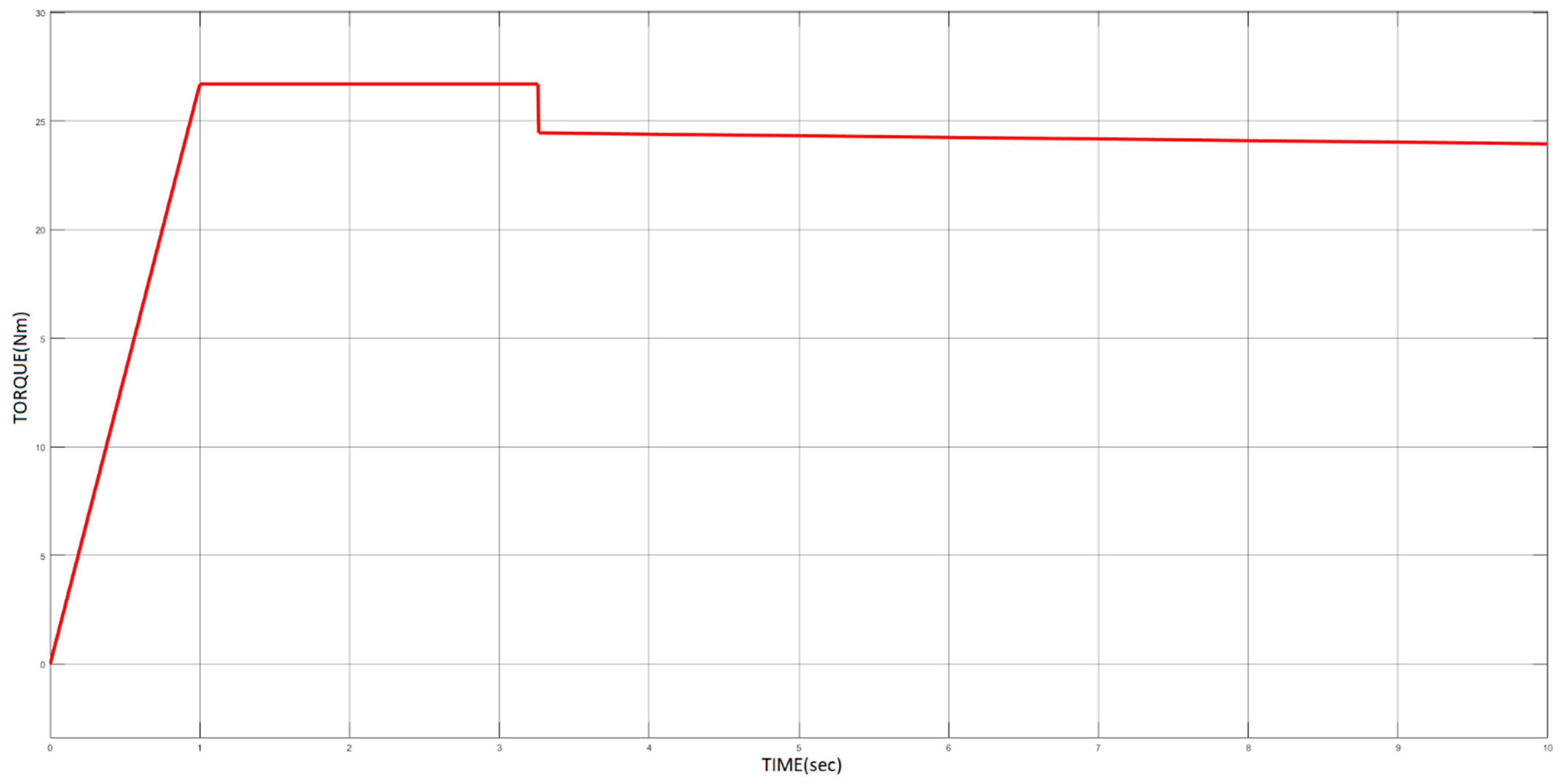
3.2. Running the Simulation

Each simulation lasted 5 s, and the sampling rate of the monitored parameters, which were the 3-phase stator’s currents, was 20.000 Hz. The IM was subjected to variable load torque that had been induced by a step function; the value, duration, and rotational speed for each load torque are summarized in

Table 2. Different load conditions of step load torque.

Duration (s)	Load Torque (Nm)	Rotational Speed (rpm)
0–1	0	1499
1–2	26.72	1434
2–3	13.36	1468
3–4	6.68	1484
4–5	0	1499

. The time series of the 3-phase currents of the stator during healthy operation are depicted in Figure 2, and the maximal current flowed during the maximal load torque. When there was a change in the load, there was a proportional change in the waveforms of the currents, as expected. The time series of the 3-phase currents of the stator during faulty operation are depicted in Figure 3, where we can easily distinguish that the operation was faulty from 1.4 to 1.7 s. Our ultimate goal was to develop a method for both the accurate and automated condition monitoring of power systems. The research methodology that is presented in Section 4 was utilized for the diagnosis of stator winding faults.

4. Research Methodology

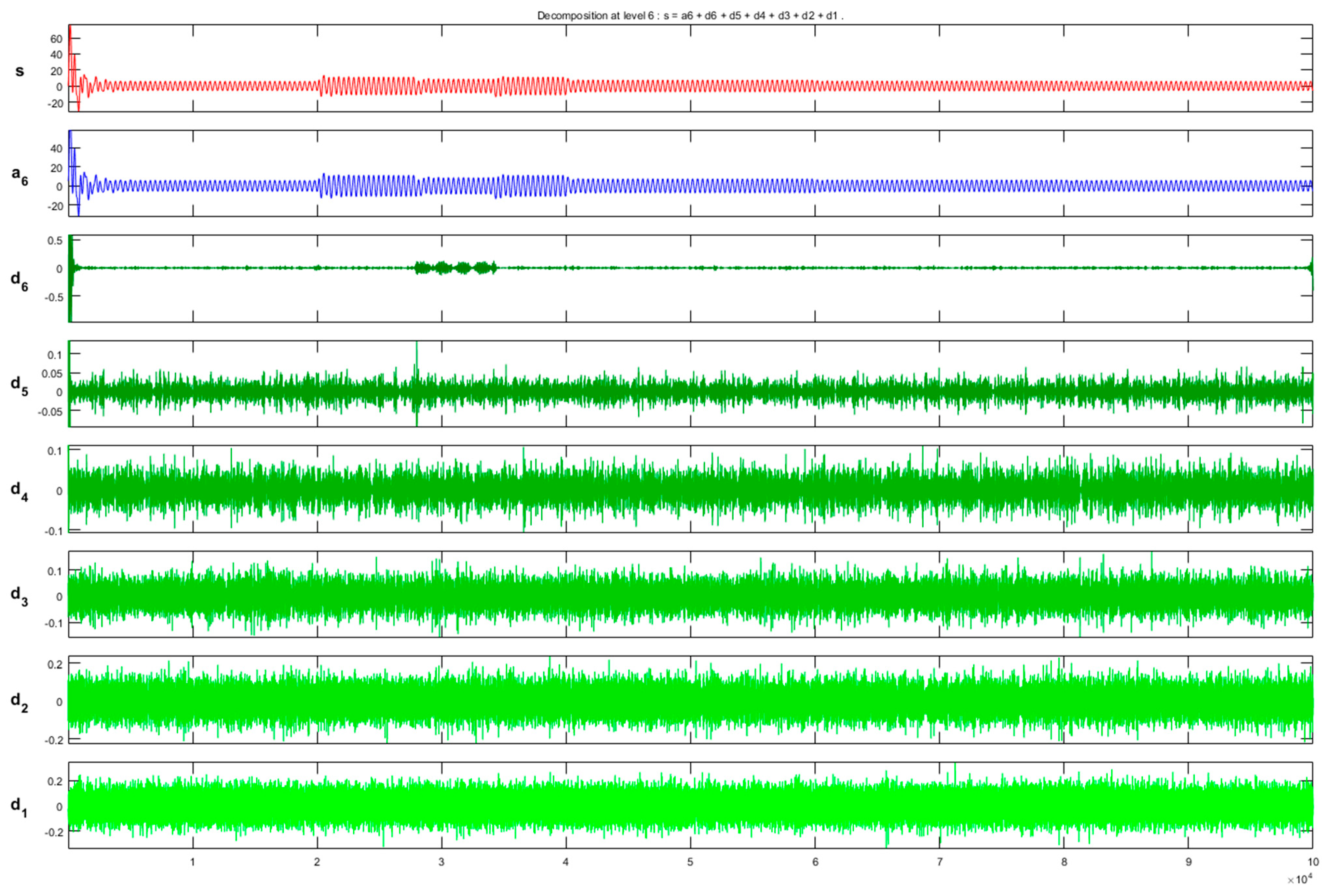
4.1. Discrete Wavelet Analysis

There are several types of wavelet transformations, each with its own set of applications, but the two main ones are continuous wavelet transform (CWT) and discrete wavelet transform (DWT), as highlighted in [9,12,24]. The CWT is mathematically expressed with the following equation [24]:

$$W\left(a, b\right)=\frac{1}{\sqrt{a}}\underset{-\infty }{\overset{+\infty }{{\displaystyle \int }}}f\left(x\right)\phi \left(\frac{x-b}{a}\right)dx$$

(1)

where $\varphi$ is the mother wavelet, $a$ is the scale factor, and $b$ is the translation factor. The values of the factors are continuous, which means that there is an infinite number of wavelets. The main difference of DWT is that discrete values are used for the scale and translation factors. DWT is mathematically expressed with the following equation [24]:

$$W\left(a, b\right)=2^{-\left(\frac{a}{2}\right)}{\displaystyle \sum }_{t=0}^{T-1}f\left(t\right)\phi \left(\frac{t-b{2}^a}{2^a}\right)$$

(2)

DWT can be utilized as a filter bank, meaning that the signal is decomposed into several frequency sub-bands (Stephane Mallat multidecomposition theory). According to the authors of [9], the DWT is implemented by convoluting the signal with sub-band low- and high-pass filters. The output of the filters returns the DWT coefficients. Decomposition theory is applied to many levels. At the first level, the signal is split into a high- and a low-frequency part to analyze it at its maximal frequency. At the second level, the previous low-frequency part is again split into high- and low-frequency parts in order to analyze it at half of its maximal frequency. This process is repeated until the maximal decomposition level, ending up with a set of approximation and detail coefficients from each level. The coefficients can be used to reconstruct the original signal.

In some cases, it is desirable to exclude detail coefficients from various levels to reconstruct the original signal without the high-frequency behavior (denoising). Harmonic frequencies are generated during faulty operation in the current; thus, in our case, it was desirable to reconstruct the original signal by keeping the detail coefficients from the appropriate levels at which faulty operation was indicated if it existed. Additionally, the selection of the appropriate mother wavelet for signal representation is crucial. There are several DWT families and they are categorized on the basis of the features of the produced basis functions. Examples of different families are Haar, the discrete approximation of Meyer, Symlet, and Daubechies.

There were cases in our simulation where the fault was indistinguishable in the time series of the currents (Figure 4). DWT was utilized to solve this problem since it is ideal for the analysis of nonstationary signals [5]. As mentioned above, the selection of an appropriate type of Wavelet is significant. In addition, the level of decomposition is important for the efficient implementation of the DWT. Reconstructed signals from various detail coefficients are depicted in Figure 5 for the case of an indistinguishable fault in the time series. On the basis of the descriptive analysis in Figure 5 and after experimenting with various types of DWT, we concluded that the discrete approximation of Meyer (Dmey) was a good option. Dmey is ideal for the computation of fast discrete wavelet transforms and it does not exhibit many disadvantages compared to other DWT types [25]. Moreover, we decided to focus on the results of the reconstructed signals from the detail coefficients of Level 5 (d5) since higher levels add unnecessary complexity, as depicted in Figure 5. Diagnosis using DWT was successful since the harmonic frequencies of the fault were captured. The MATLAB Wavelet Toolbox was used for the implementation of DWT analysis.

4.2. Convolutional Neural Networks

Convolutional neural networks (CNNs) are similar to ANNs since they are composed of neural networks, but they include some distinctive features, which are the convolutional and pooling layers. Convolution acts as a sliding filter and it was first introduced by Kunihiko Fukushima [26] back in 1980. Researchers utilize CNN to cope with challenging problems that are mainly divided into two main categories: (1) computer vision tasks with 2D input data such as image classification, object detection, and image segmentation; (2) sequential problems with 1D input data such as time series forecasting, time series classification, and natural language processing. The power of CNNs lies in extracting valuable regional information. Furthermore, they are more effective to search for features in smaller portions rather than the entire data. The structure of a 1D CNN consists of three basic types of layers: 1D convolutional and 1D pooling layers for feature extraction, and fully connected layers for the final decision. The 1D CNN operation is briefly explained below, as described in our previous work [8]:

First, raw 1D input vector $x\left[n\right]$ is fed into a 1D convolutional layer. Output $f\left[n\right]$ is called the feature map and it is calculated as in (3).

$$f\left[n\right]=x\left[n\right]\ast k\left[n\right]={{\displaystyle \sum }}_{m=0}^{w-1}k\left[m\right]x\left[n-m\right]$$

(3)

Equation (3) is a linear elementwise multiplication, and the filters of kernels $\kappa \left[n\right]$ are convolved with $x\left[n\right]$ to produce feature map $f\left[n\right]$. The most important parameter is the size of the kernel, expressed as $w$, because it defines the size of the feature map [8].

The feature map of the convolutional operation is fed into a nonlinear activation function, expressed as $F$, to produce output $Z\left(n\right)$ on the basis of Equation (4). A common activation function was sigmoid, but gradient vanishing problems during back-propagation prompted researchers to investigate alternative activation functions according to the authors of [8]. One of the most promising is rectifier linear unit (ReLU), expressed as in (5).

$$Z\left(n\right)=F\left(f\left(n\right)\right)$$

(4)

$$ReLU\left(x\right)=\max \left(0,\mathrm{x}\right)$$

(5)

The output of the activated convolutional layer is then fed into a pooling layer, aiming at decreasing computational costs. There is a variety of pooling operations, but 1D max pooling is a good option [27]. A window, such as the kernel stated in the convolutional layer, slides through the activated feature map to keep only the maximal values while discarding all other information.

Many convolutional and pooling layers could be combined for a final output feature map. A special layer flattens the output, which is then fed into some fully connected layers. The fully connected layers follow the ANN structure. To overcome problems of overfitting, a dropout layer is implemented in many cases. This layer drops some neurons from the neural network during the training process. Lastly, depending on the task, the number of neurons and the type of activation function of the final dense layer must be chosen wisely. For a 3-class classification task, the dense layer is expressed as in (6).

$$a^{\left[L\right]}=Softmax(W^T{a}^{\left[L-1\right]}+b)$$

(6)

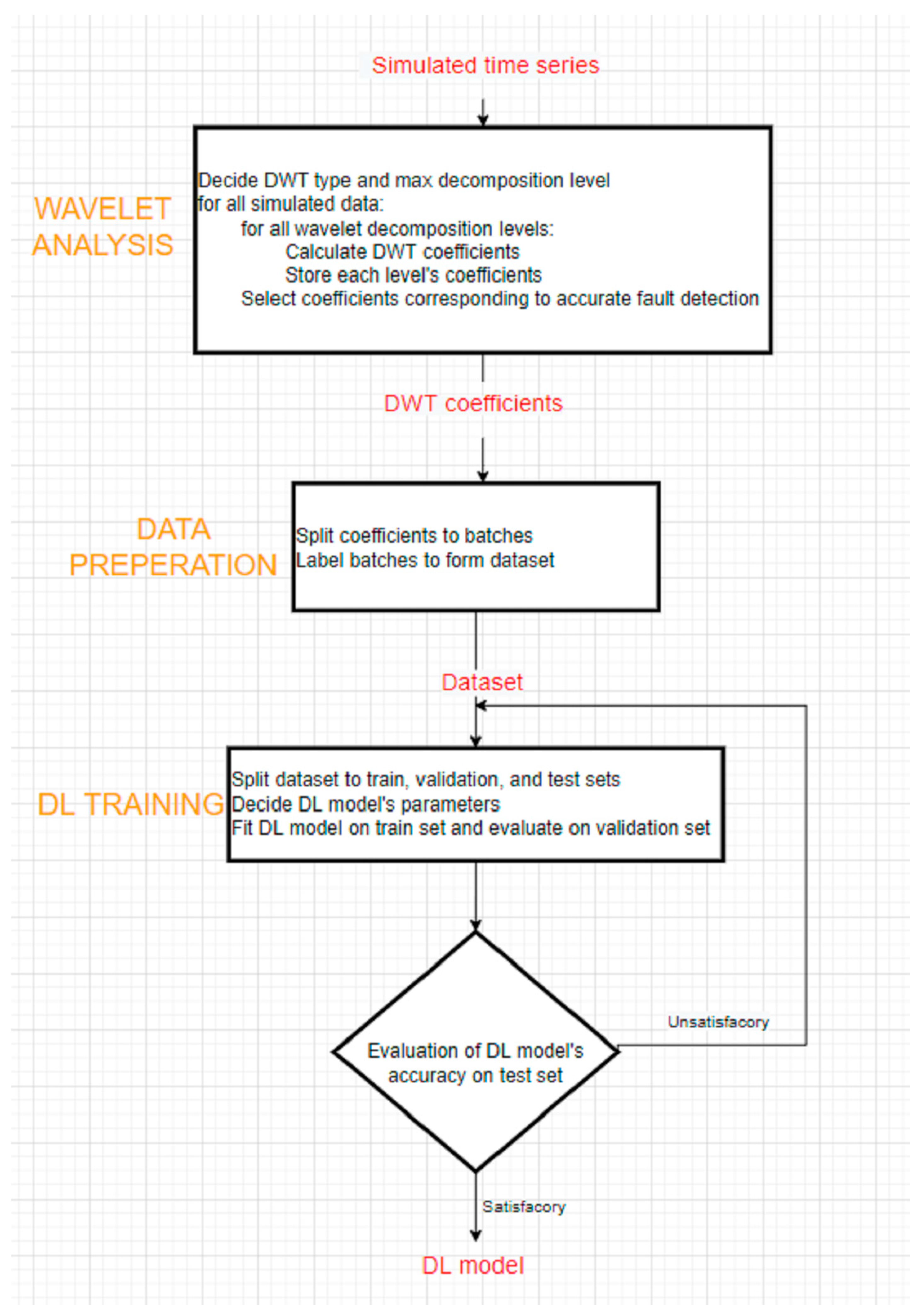
4.3. Hybrid Discrete Wavelet–CNN Method

The hybrid method consists of two main blocks, DWT analysis and a CNN model. For concluding an inference model, it is necessary to train the model with pairs of batches of DWT-analyzed signals and the corresponding labels for normal and faulty operation. The DWT analysis block is utilized for the feature extraction of valuable information from the time series. The features could be generated from the coefficients of each level. In more detail, these features could be statistical values, such as variance, standard deviation, mean, median, and the 70th percentile or just the raw values of the coefficients. Data preparation is needed to prepare a training dataset that is employed to train a CNN model.

5. Results

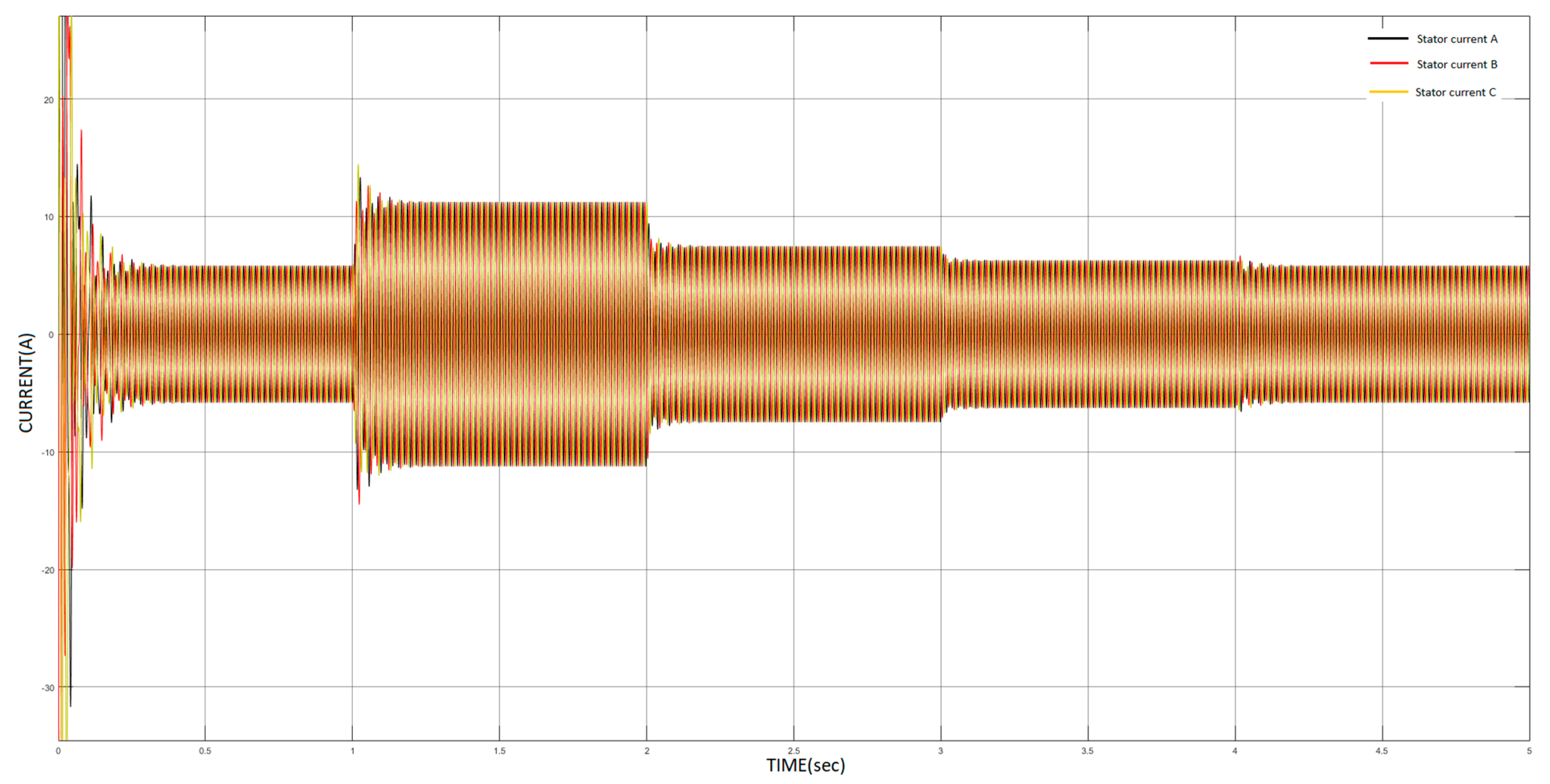
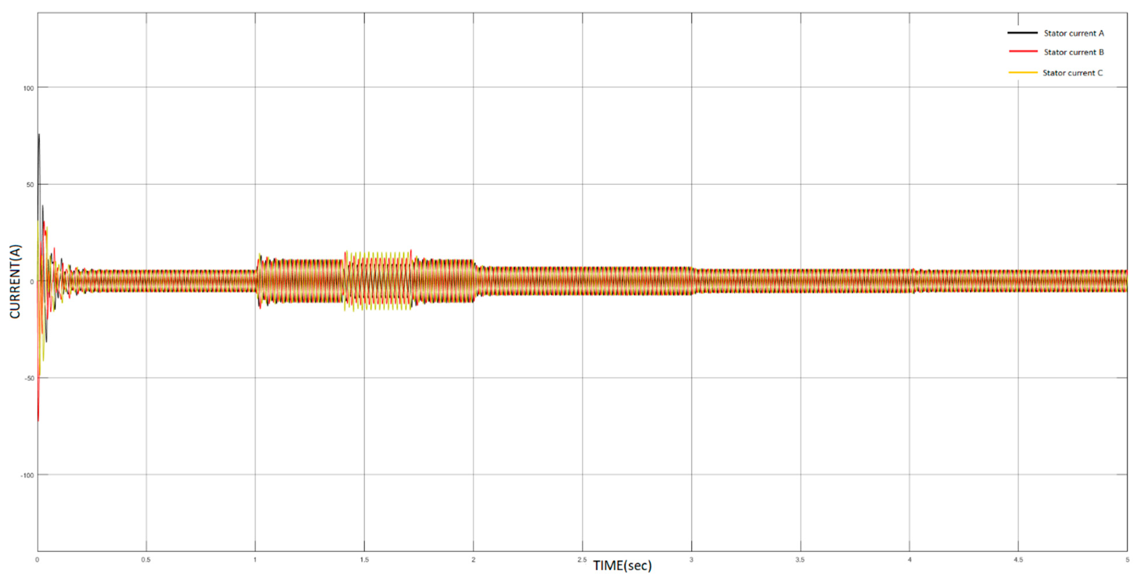
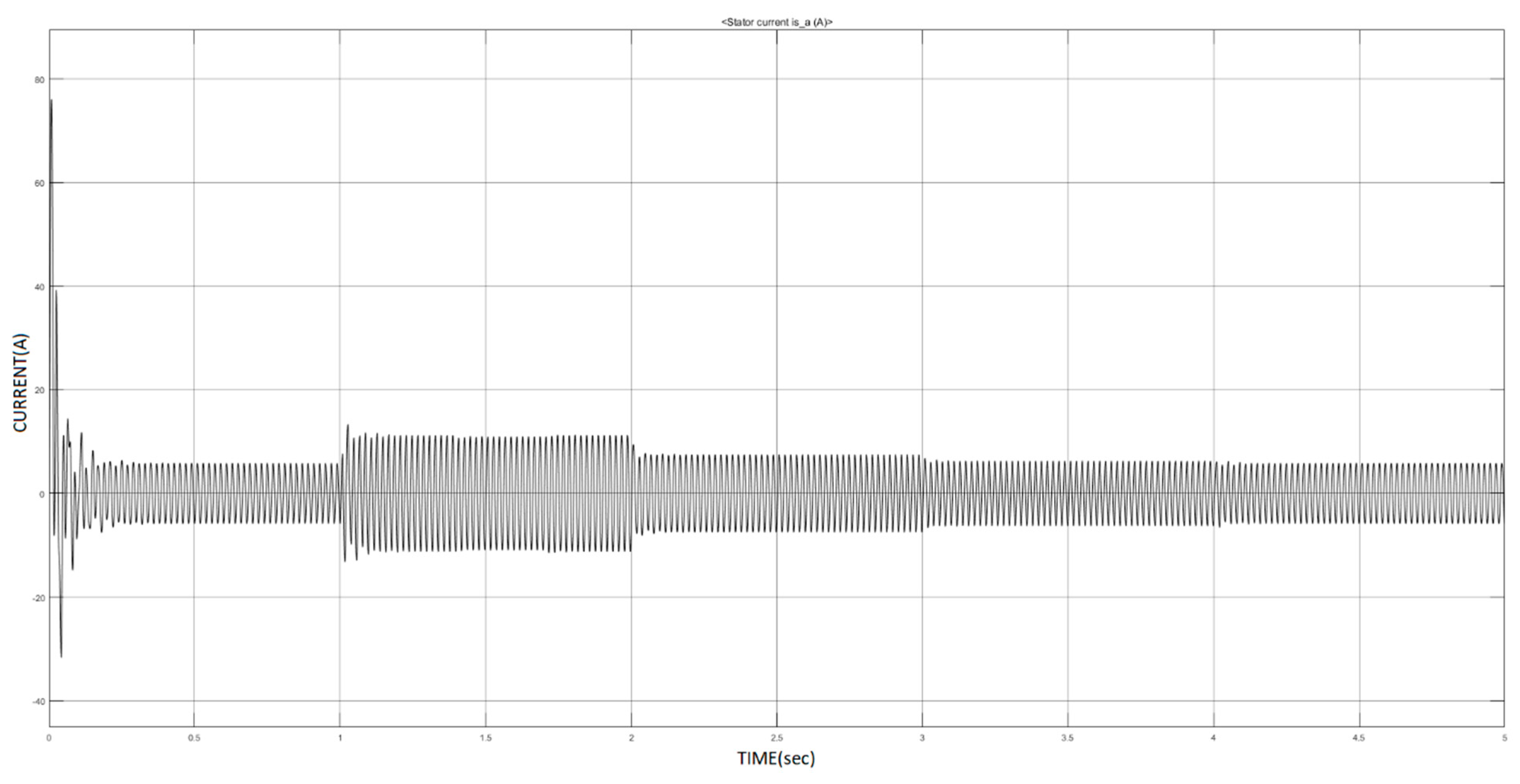
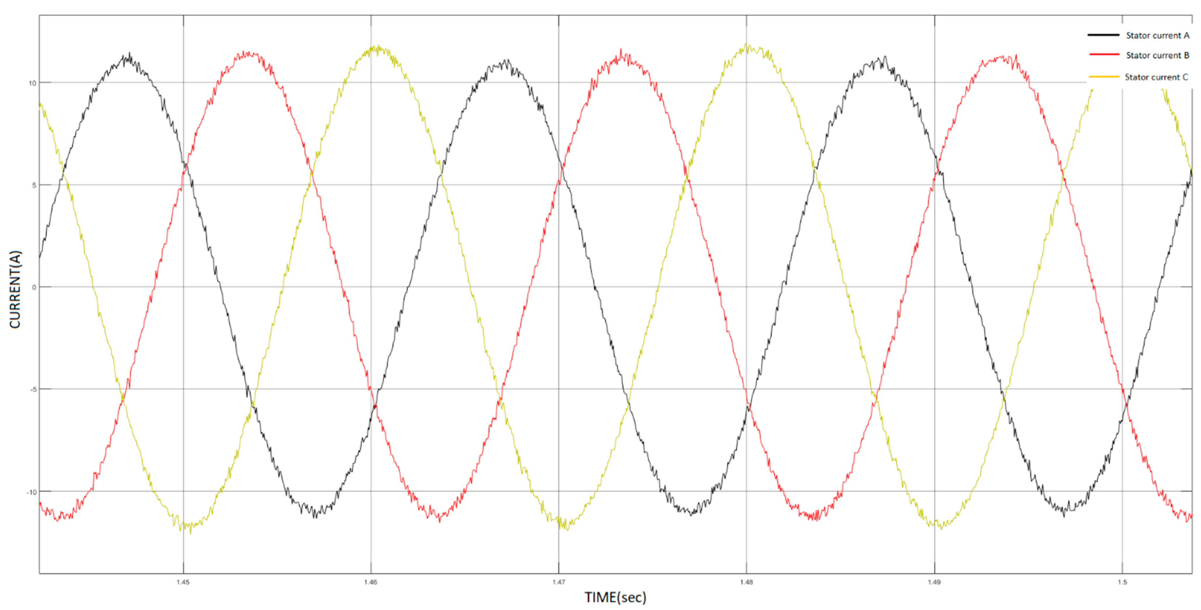
5.1. Descriptive Analysis

This subsection presents a descriptive analysis for the diagnosis of various faults using DWT. The time series of the currents were generated from various cases of simulations, and DWT was then applied to them. The various cases included different:

• Types of short circuits (A–B, A–G, A–C, etc.).
• Intensities of fault, controlled by the fault resistance (R).
• Moments of fault.
• Scales of white noise (W-N) (Figure 6).
• Load conditions (Table 2).

Additionally, there were simulations with the ramp load torque (Figure 7).

There was a level for every fault detection case depending on how easy it was to identify the fault. In total, there were 5 levels, as presented in

Table 3. Five levels of diagnosis.

Threshold	d5	Many d	Indistinguishable	Unrecognizable
Level 1	Level 2	Level 3	Level 4	Level 5

. In the Level 1 cases, the comparison with a threshold value was sufficient to detect the fault in d5. The threshold was calculated from the reconstructed range of d5 during healthy operation (

Table 4. Threshold value.

Phase A	Phase B	Phase C
0.01137	0.012	0.019

). In the Level 2 cases, the fault was identified in d5, while in Level 3, the fault could not be identified in d5, and it was necessary to observe many levels of detail coefficients. In Level 4, it was extremely difficult to identify the fault from any level of detail coefficients. Lastly, in Level 5, it was unrecognizable. The results of the analysis for each monitoring parameter (3-phase currents) are summarized in

Table 5. Operation with fault at 1.4–1.7 s for the step load toque.

Monitoring Parameter	Type	Intensity R (Ω)	Level
Current of Phase A	A–B	0.1	1
	A–G	0.1	1
	A–C	0.1	1
	B–C	0.1	2
	B–G	0.1	1
	C–G	0.1	1
	A–B	1.0	1
	A–G	1.0	3
	A–B	5.0	3
	A–G	5.0	4
Current of Phase B	A–B	0.1	1
	A–G	0.1	1
	A–C	0.1	3
	B–C	0.1	1
	B–G	0.1	1
	C–G	0.1	1
	A–B	1.0	1
	A–G	1.0	5
	A–B	5.0	3
	A–G	5.0	5
Current of Phase C	A–B	0.1	3
	A–G	0.1	3
	A–C	0.1	1
	B–C	0.1	1
	B–G	0.1	1
	C–G	0.1	1
	A–B	1.0	5
	A–G	1.0	4
	A–B	5.0	5
	A–G	5.0	5

,

Table 6. Operation with fault at 1.9–2.2 s for step load torque.

Monitoring Parameter	Type	Intensity R (Ω)	Level
Current of Phase A	A–B	0.1	1
	A–G	0.1	1
Current of Phase B	A–B	0.1	1
	A–G	0.1	3
Current of Phase C	A–B	0.1	3
	A–G	0.1	3

and

Table 7. Operation with fault at 1.4–1.7 s for step load torque and W–N = 60 Eb/No.

Monitoring Parameter	Type	Intensity R (Ω)	Level
Current of Phase A	A–B	0.1	1
	A–G	0.1	4
Current of Phase B	A–B	0.1	1
	A–G	0.1	5
Current of Phase C	A–B	0.1	4
	A–G	0.1	4

for the step load torque, and in

Table 8. Operation with fault at 1.4–1.7 s for ramp load torque.

Monitoring Parameter	Type	Intensity R (Ω)	Level
Current of Phase A	A–B	5.0	2
	A–G	5.0	4
Current of Phase B	A–B	5.0	3
	A–G	5.0	5
Current of Phase C	A–B	5.0	5
	A–G	5.0	4

and

Table 9. Operation with fault at 1.4–1.7 s for ramp load torque and W–N = 60 Eb/No.

Monitoring Parameter	Type	Intensity R (Ω)	Level
Current of Phase A	A–B	0.1	1
	A–G	0.1	3
Current of Phase B	A–B	0.1	1
	A–G	0.1	3
Current of Phase C	A–B	0.1	3
	A–G	0.1	4

for the ramp load torque.

Some limitations exist with the descriptive analysis using DWT. The fault was hardly detected in cases where there was W–N in the time series (Figure 8). Figure 8 depicts reconstructed signal from the detail coefficients of levels 1–6 (d1–d6), the reconstructed signal from the approximate coefficients of level 6 (a6), and the original signal (s). The fault was unrecognizable in cases with a nonintense fault (R5.0). Moreover, it was indistinguishable whether a frequency had been caused by a load change or by a fault in some cases. The classification of the fault type (A–B, A–G, B–C) could not be achieved. In the next subsection, we show how our hybrid method was implemented to tackle the limitations.

5.2. Hybrid Discrete Wavelet–CNN Model

The hybrid discrete wavelet–CNN model recognizes if the operation of IM is healthy or faulty on the basis of the analyzed DWT current of Phase A. It was also trained to recognize two types of fault (A–B and A–G short circuits); thus, it is considered a 3-class classifier. It is crucial that our trained hybrid model does not have problems with overfitting. Overfitting means that the model is excellent at recognizing faults in a training set, but is not capable of recognizing them in cases outside of the distribution of the training set. Therefore, the time series were processed from various simulations. The hybrid discrete wavelet–CNN method was implemented in Python.

5.2.1. Training Parameters

The training process of the hybrid discrete wavelet–CNN model is depicted in pseudocode form in Figure 9. First, the time series of Current A were analyzed using DWT with the efficient Dmey wavelet. Then, the raw values of detail coefficients of Level 5 were extracted. The samples of the time series were 100,000, while the samples of the batches were 1562 after DWT analysis. In this way, the data were compressed without losing information, and the training time of CNN model was extremely shorter. The model’s architecture is presented in

Table 10. Proposed neural network architecture.

Layer	Number	Parameters
Conv1D	2	Filters = 64, kernel size = 3, activation = ReLU.
Dropout	1	Rate = 0.5.
MaxPooling1D	1	Pool size = 2.
Flatten Dense 1	1 1	- Units = 100, activation = ReLU.
Dense 2	1	Units = 3, activation = softmax.

, and the hyperparameters employed for training were as follows:

• Epochs = 100.
• Batch size = 4.
• Learning rate = 0.001.
• Optimizer = ADAM.
• Dataset split = 70%, 15%, 15%.

5.2.2. Results

After every iteration, the model was evaluated in the validation set to verify its accuracy. Figure 10a depicts both training and validation accuracy, while Figure 10b depicts the desirable loss reduction. The trained model was implemented for predictions in the test set, and its predictions were correct in all cases. Figure 11 depicts the confusion matrix of the model, and the results of the matrix were distributed on the diagonal, which means that the introduced model predicted only true positives and true negatives.

5.3. Discussion

The custom fault-detection challenge-indicative levels from Table 5, Table 6, Table 7, Table 8 and Table 9 show that the harmonic frequencies of the faults were captured in most cases, providing valuable initial information, but there were cases where it was extremely difficult to diagnose nonintense faults, especially in noisy simulated data. Furthermore, the appropriate selection of the mother wavelet and the level of decomposition are key factors for this particular application. After feature extraction using DWT, the power of 1D CNN models was utilized to complete the novel hybrid discrete wavelet–CNN model.

A main distinction of our research compared to related works is that the currents were obtained from simulations that included various load conditions, types, intensities of faults, and scales of white noise. The combination of 1D CNN and DWT is the other distinction of our research, and it was employed to automatically diagnose even more indistinguishable and complex faults. The proposed method could also be considered the first step towards the development of a complete diagnostic system that is able to detect and predict all types of IM faults from transfer learning on the basis of simulation data, and able to be implemented to reduce the training costs of experimental analysis.

6. Conclusions

The related works mentioned in Section 2 involved only a few proposed methods related to wavelet techniques in coordination with DL. Additionally, there is a strong interest to diagnose faults adequately early when the current exceeds the rated amperage capacity of the circuit of the connected equipment since, in cases of failure faults, the power system could be damaged, and the health of human operators could be threatened. The present work introduced a hybrid wavelet–CNN and a corresponding method for current analysis to diagnose stator winding faults of 3-phase IMs; its main contributions are as follows:

• It can automatically and effectively classify faults related to short circuits even in indistinguishable cases where white noise and load changes occur.
• It can drastically reduce both the training time and the data volume employed for training the neural network while maintaining competitive accuracy. Therefore, the proposed method could be considered a data compression method as well.

In contemporary sensor network applications that often include mist and edge computing systems with limited processing power and storage capabilities, reductions in model training time and data volume are crucial.

Future work will be conducted to test the hybrid method with experimental data of IM operation to verify the system’s accuracy. We are also interested in testing the method for fault detection in a variety of other applications and classifying several types of faults. An example is the thermographic fault diagnosis of motor shafts. Lastly, possible future work could involve its implementation to other power systems, including power transformers, power generators, and other types of motors, such as brushless DC electric and permanent-magnet motors.

References

1. Albrecht, P.F.; Appiarius, J.C.; McCoy, R.M.; Owen, E.L.; Sharma, D.K. Assessment of the Reliability of Motors in Utility Applications—Updated. IEEE Power Eng. Rev. 1986, PER-6, 31–32. [Google Scholar] [CrossRef]
2. Singh, G.K.; Al Kazzaz, S.A.S. Induction machine drive condition monitoring and diagnostic research—A survey. Electr. Power Syst. Res. 2003, 64, 145–158. [Google Scholar] [CrossRef]
3. Karmakar, S.; Chattopadhyay, S.; Mitra, M.; Sengupta, S. Induction Motor and Faults. In Induction Motor Fault Diagnosis. Power Systems; Springer: Singapore, 2016; pp. 7–28. [Google Scholar] [CrossRef]
4. Mortazavizadeh, S. A Review on Condition Monitoring and Diagnostic Techniques of Rotating Electrical Machines. Phys. Sci. Int. J. 2014, 4, 310–338. [Google Scholar] [CrossRef]
5. Laamari, Y.; Allaoui, S.; Bendaikha, A.; Saad, S. Fault Detection Between Stator Windings Turns of Permanent Magnet Synchronous Motor Based on Torque and Stator-Current Analysis Using FFT and Discrete Wavelet Transform. Math. Model. Eng. Probl. 2021, 8, 315–322. [Google Scholar] [CrossRef]
6. Theodoropoulos, P.; Spandonidis, C.C.; Fassois, S. Use of Convolutional Neural Networks for vessel performance optimization and safety enhancement. Ocean Eng. 2022, 248, 110771. [Google Scholar] [CrossRef]
7. Spandonidis, C.; Theodoropoulos, P.; Giannopoulos, F.; Galiatsatos, N.; Petsa, A. Evaluation of deep learning approaches for oil & gas pipeline leak detection using wireless sensor networks. Eng. Appl. Artif. Intell. 2022, 113, 104890. [Google Scholar] [CrossRef]
8. Theodoropoulos, P.; Spandonidis, C.C.; Giannopoulos, F.; Fassois, S. A Deep Learning-Based Fault Detection Model for Optimization of Shipping Operations and Enhancement of Maritime Safety. Sensors 2021, 21, 5658. [Google Scholar] [CrossRef]
9. Jayaswal, P.; Wadhwani, A.K. Application of artificial neural networks, fuzzy logic and wavelet transform in fault diagnosis via vibration signal analysis: A review. Aust. J. Mech. Eng. 2009, 7, 157–171. [Google Scholar] [CrossRef]
10. Verma, A.K.; Nagpal, S.; Desai, A.; Sudha, R. An efficient neural-network model for real-time fault detection in industrial machine. Neural Comput. Appl. 2021, 33, 1297–1310. [Google Scholar] [CrossRef]
11. Duan, L.; Hu, J.; Zhao, G.; Chen, K.; Wang, S.X.; He, J. Method of inter-turn fault detection for next-generation smart transformers based on deep learning algorithm. High Volt. 2019, 4, 282–291. [Google Scholar] [CrossRef]
12. Ashfaq, H.; Quadri, M.N. Fault Current Detection of Three Phase Power Transformer Using Wavelet Transform. J. Eng. Res. Appl. 2013, 3, 1444–1454. [Google Scholar]
13. Hussain, M.; Soother, D.K.; Kalwar, I.H.; Memon, T.D.; Memon, Z.A.; Nisar, K.; Chowdhry, B.S. Stator winding fault detection and classification in three-phase induction motor. Intell. Autom. Soft Comput. 2021, 29, 869–883. [Google Scholar] [CrossRef]
14. Hsueh, Y.-M.; Ittangihal, V.R.; Wu, W.-B.; Chang, H.-C.; Kuo, C.-C. Fault Diagnosis System for Induction Motors by CNN Using Empirical Wavelet Transform. Symmetry 2019, 11, 1212. [Google Scholar] [CrossRef]
15. Wang, J.; Zhuang, J.; Duan, L.; Cheng, W. A multi-scale convolution neural network for featureless fault diagnosis. In Proceedings of the 2016 International Symposium on Flexible Automation (ISFA), Cleveland, OH, USA, 1–3 August 2016; pp. 65–70. [Google Scholar] [CrossRef]
16. Agrawal, P.; Jayaswal, P. Diagnosis and Classifications of Bearing Faults Using Artificial Neural Network and Support Vector Machine. J. Inst. Eng. Ser. C 2020, 101, 61–72. [Google Scholar] [CrossRef]
17. Yan, X.; She, D.; Xu, Y. Deep order-wavelet convolutional variational autoencoder for fault identification of rolling bearing under fluctuating speed conditions. Expert Syst. Appl. 2023, 216, 119479. [Google Scholar] [CrossRef]
18. Attallah, O.; Ibrahim, R.A.; Zakzouk, N.E. Fault diagnosis for induction generator-based wind turbine using ensemble deep learning techniques. Energy Rep. 2022, 8, 12787–12798. [Google Scholar] [CrossRef]
19. Mansour, R.F.; Alabdulkreem, E.; Eid, H.F.; K, S.; Khan, M.A.R.; Kumar, A. Fuzzy logic based on-line fault detection and classification method of substation equipment based on convolutional probabilistic neural network with discrete wavelet transform and fuzzy interference. Optik 2022, 270, 169956. [Google Scholar] [CrossRef]
20. Tang, S.; Zhu, Y.; Yuan, S. Intelligent fault identification of hydraulic pump using deep adaptive normalized CNN and synchrosqueezed wavelet transform. Reliab. Eng. Syst. Saf. 2022, 224, 108560. [Google Scholar] [CrossRef]
21. Ahmadipour, M.; Othman, M.M.; Alrifaey, M.; Bo, R.; Ang, C.K. Classification of faults in grid-connected photovoltaic system based on wavelet packet transform and an equilibrium optimization algorithm-extreme learning machine. Meas. J. Int. Meas. Confed. 2022, 197, 111338. [Google Scholar] [CrossRef]
22. Allan, O.A.; Morsi, W.G. A new passive islanding detection approach using wavelets and deep learning for grid-connected photovoltaic systems. Electr. Power Syst. Res. 2021, 199, 107437. [Google Scholar] [CrossRef]
23. Venkatesh, S.N.; Jeyavadhanam, B.R.; Sizkouhi, A.M.; Esmailifar, S.; Aghaei, M.; Sugumaran, V. Automatic detection of visual faults on photovoltaic modules using deep ensemble learning network. Energy Rep. 2022, 8, 14382–14395. [Google Scholar] [CrossRef]
24. Esfetanaj, N.N.; Nojavan, S. The Use of Hybrid Neural Networks, Wavelet Transform and Heuristic Algorithm of WIPSO in Smart Grids to Improve Short-Term Prediction of Load, Solar Power, and Wind Energy. In Operation of Distributed Energy Resources in Smart Distribution Networks; Elsevier: Amsterdam, The Netherlands, 2018; pp. 75–100. [Google Scholar] [CrossRef]
25. Guo, T.; Zhang, T.; Lim, E.; Lopez-Benitez, M.; Ma, F.; Yu, L. A Review of Wavelet Analysis and Its Applications: Challenges and Opportunities. IEEE Access 2022, 10, 58869–58903. [Google Scholar] [CrossRef]
26. Fukushima, K. Neocognitron: A self-organizing neural network model for a mechanism of pattern recognition unaffected by shift in position. Biol. Cybern. 1980, 36, 193–202. [Google Scholar] [CrossRef]
27. Cordeiro, J.R.; Raimundo, A.; Postolache, O.; Sebastião, P. Neural Architecture Search for 1D CNNs—Different Approaches Tests and Measurements. Sensors 2021, 21, 7990. [Google Scholar] [CrossRef]
Figure 1. Simulation model in MATLAB Simulink.
Signals 04 00008 g001
Figure 2. Time series of 3–phase stator currents during healthy operation.
Signals 04 00008 g002
Figure 3. Time series of 3–phase stator currents during faulty operation.
Signals 04 00008 g003
Figure 4. Time series of Current A during unrecognizable faulty operation.
Signals 04 00008 g004
Figure 5. Reconstructed signals of Current A using DWT during unrecognizable faulty operation.
Signals 04 00008 g005
Figure 6. Time series of currents with induced W–N.
Signals 04 00008 g006
Figure 7. Ramp load toque of IM.
Signals 04 00008 g007
Figure 8. Reconstructed W–N signals using DWT.
Signals 04 00008 g008
Figure 9. Pseudocode of the training process.
Signals 04 00008 g009
Figure 10. (a) Accuracy and (b) loss curves over 100 epochs of CNN training.
Signals 04 00008 g010
Figure 11. Confusion matrix of the model.
Signals 04 00008 g011