Transmission Line Fault Classification of Multi-Dataset Using CatBoost Classifier

Abstract

Transmission line fault classification forms the basis of fault protection management in power systems. Because faults have adverse effects on transmission lines, adequate measures must be implemented to avoid power outages. This paper focuses on using the categorical boosting (CatBoost) algorithm classifier to analyse and train multiple voltage and current data from a 330 kV and 500 km-long simulated faulty transmission line model designed using Matlab/Simulink. From it, 93,340 fault data sizes were extracted. The CatBoost classifier was employed to classify the faults after different machine learning algorithms were used to train the same data with different parameters. The trainer achieved the best accuracy of 99.54%, with an error of 0.46% for 748 iterations out of 1000. The algorithm was selected for its high performance in classifying faults based on accuracy, precision and speed. In addition, it is easy to use and handles multiple data-sets. In contrast, a support vector machine and an artificial neural network each has a longer training time than the proposed method’s 58.5 s. Proper fault classification techniques assist in the effective fault management and planning of power system control thereby preventing energy waste and providing high performance.

1. Introduction

An electrical power system consists of different interacting segments: generation, transmission, and distribution. The transmission line is an integral part since it transfers electricity from the generating station to the distribution network and to the end-user. These components are interconnected through the transmission lines, which are subject to faults and cannot be controlled manually except through advanced techniques [1]. When a fault occurs, significant damage is done to the power system’s reliability, affecting power output and causing loss of installations, outages, and system collapse. It is imperative that a model be designed that can classify and locate a fault quickly and precisely so that it can be isolated and identified for fault protection and management.

Fault classification is essential for protecting the network; therefore, measures must be taken to achieve maximum protection to avert system collapse and preserve energy output. Faults can be categorised as incipient or unpredictable [2]. Incipient faults are transient, while unpredictable faults occur due to human interference, lightning, and extreme weather, which directly affect the entire network.

Researchers in recent years have been brainstorming the best way to protect transmission lines from faults, which must be classified according to type to isolate the line quickly and prevent system collapse [3]. However, feedback generated from fault classification can significantly assist in detecting a fault location so that power can be restored quickly [4]. The recent literature has discussed fault classification using machine learning: an artificial neural network (ANN) [5,6,7,8,9], support vector machine (SVM), [1,2,10], decision tree (DT) [11] and probabilistic neural network (PNN) [12].

All these methods have been used for the classification of faults. However, some, like the wavelet technique (WT), are helpful when time and frequency data are needed although this technique is sensitive to noise and harmonics, and requires a high sampling rate. It is time-consuming because getting a referred wavelet and the number of decompositions is done by trials. Although WT detects faults accurately and instantly, it is has trouble differentiating among various fault conditions [12]. WT and ANN are predominantly used for fault detection and classification [13].

Many hybrid methods have produced good results. S-transform and ANNs were used to classify faults on the transmission line. Though the ANN and SVM produced good results in identifying faults, they needed a large volume of data for training, making them complex to handle [14]. Furthermore, in [12], three ANN approaches were compared to each other for fault classification: PNN, Back Propagation Neural Network (BPNN) and Radial Basis Function Neural Network (RBFNN). These methods produced accurate results, but they were used on faulty voltage and current signals and focused more on time and speed of execution of the training. Despite the fact that most of these methods have been used recently, there are some challenges, such as not being applicable for high-frequency signals and high computational complexity, as found in the Hilbert–Huang Transform (HHT) [15]. The convolutional neural network (CNN) is another technique used in fault classification that is accurate and fast, but the computational cost for offline analysis is relatively high [16]. Principal Component Analysis (PCA) in machine learning is a fast and simple method that reduces re-projection error and is immune to noise. It is also used to map data from multidimensional space to low-dimensional subspace to mitigate dimensionality and perceive the variance of the data in the best way possible. The Kernel Principal Component Analysis (KPCA) and the SVM were used for the real-time fault diagnosis of a high-voltage circuit breaker, whereas a sample reduction algorithm based on a similarity degree function was used to analyse the similarity among the samples to detect faults [17] and with the dynamic kernel principal component analysis (DKPCA) [18]. However, if the number of dimensions is greater than the number of data points, the convergence matrix is always large, making it difficult to obtain a convergence matrix for data that has varying properties and capabilities [16,19].

Deep-learning diagnosis techniques, such as the wavelet packet distortion and a CNN [20], have also been used in fault classification. It applies the wavelet packet distortion to generate a faulty data sample, while the CNN is used to classify the fault into different categories. However, the wavelet packet function uses Daubechies wavelet (DB4) for extraction, which does not have a theoretical justification. The adaptive intraclass and interclass CNN (AIICNN) [21] was applied in the algorithm to enhance sample distribution differences by applying designed intraclass and interclass constraints. The 1-D CNN (1dCNN) had an added activation function to enlarge the heterogeneous and reduce the homogeneous distance between samples for proper classification. A normalized conditional variational auto-encoder with adaptive focal loss (NCVAE–AFL) was also used to classify faults into different categories [22]. In [23], the CNN long short-term memory (CNN-LSTM) was used to identify and locate a fault using the frequency response analysis (FRA) to extract it. This method detected faults accurately and in a timely manner.

Each of the methods mentioned above had disadvantages and limitations. Some of the main noticeable observations were the inability of most articles to explain fault classification extensively concerning fault clearing time, thereby making it difficult to isolate the fault or take on significant repairs within the shortest possible time. Moreover, discrete wavelet transform (DWT) and DT [24] had a limited time resolution capability and had a low performance for high-performance faults. Wavelet and Data mining [24], K-Nearest Neighbours (KNN) and Decision Tree [25], are limited to the fault classification technique but without considering the speed, accuracy and precision of the result. In [26], fault classification was not determined using the S-transform technique, and the effect of noise in the transmission line was not considered in the model [27]. Differential and Hibert–Huang transmission methods are expensive and have a no-fault direction. In addition, for fault classification, the mathematical morphology and recursive least-square (RLS) methods [28] involves using a mathematical morphology-based fault feature extraction scheme. This method has high calculation and technical standards that necessitate professional implementation.

Researchers have widely used machine learning for its increased involvement of communication and computation in transmission systems [28]. Research shows that most techniques use a smaller dataset to train the algorithm, giving highly accurate results. They also use either a single phase-to-ground fault or a double phase-to-line fault data for training [15,29,30]. Another shortcoming of most of the methods is the inability to consider the inevitable noise and disturbance in the transmission line networks. This method will also address the effect of noise signals and disturbance and how they can be reduced or eliminated for optimal system performance and accuracy of results.

Due to the shortcoming of the different algorithms and models discussed in the literature on fault classification, the CatBoost classifier algorithm is proposed for the training of fault data from single-phase, double-phase, and three phase-to-ground faults. Twelve different dataset types were used for fault classification and the CatBoost classifier was used to train the data. This classifier was proposed because of its accuracy, speed and ability to train the multi-dataset of a transmission line fault within the shortest possible time. The model was used for its ability to handle heterogeneous data and its categorical features. It was also sensitive to hyperparameters and handled noisy data [31]. The uniqueness of the proposed model is its ability to train noise data without affecting the accuracy and performance of the system. The fault data was comprised of four fault conditions in different scenarios, and the analysis was divided into two parts: one was the modelling of the network to extract fault cases from the transmission line using Matlab/Simulink, and the other was to detect and classify the faults using the data generated from the simulations to detect and classify faults with the help of a trained classifier [32].

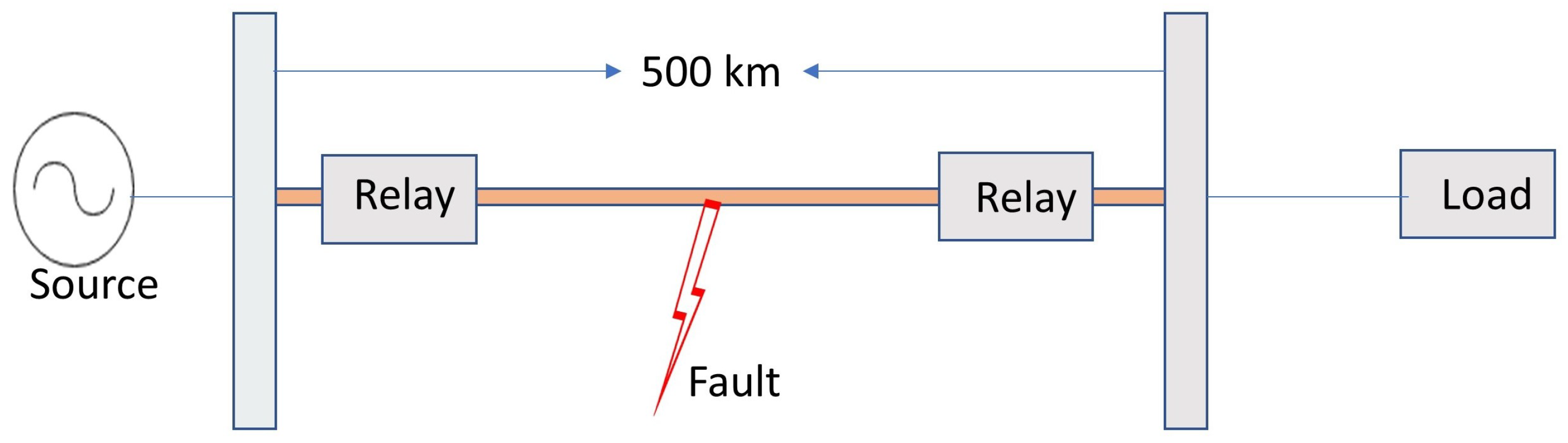
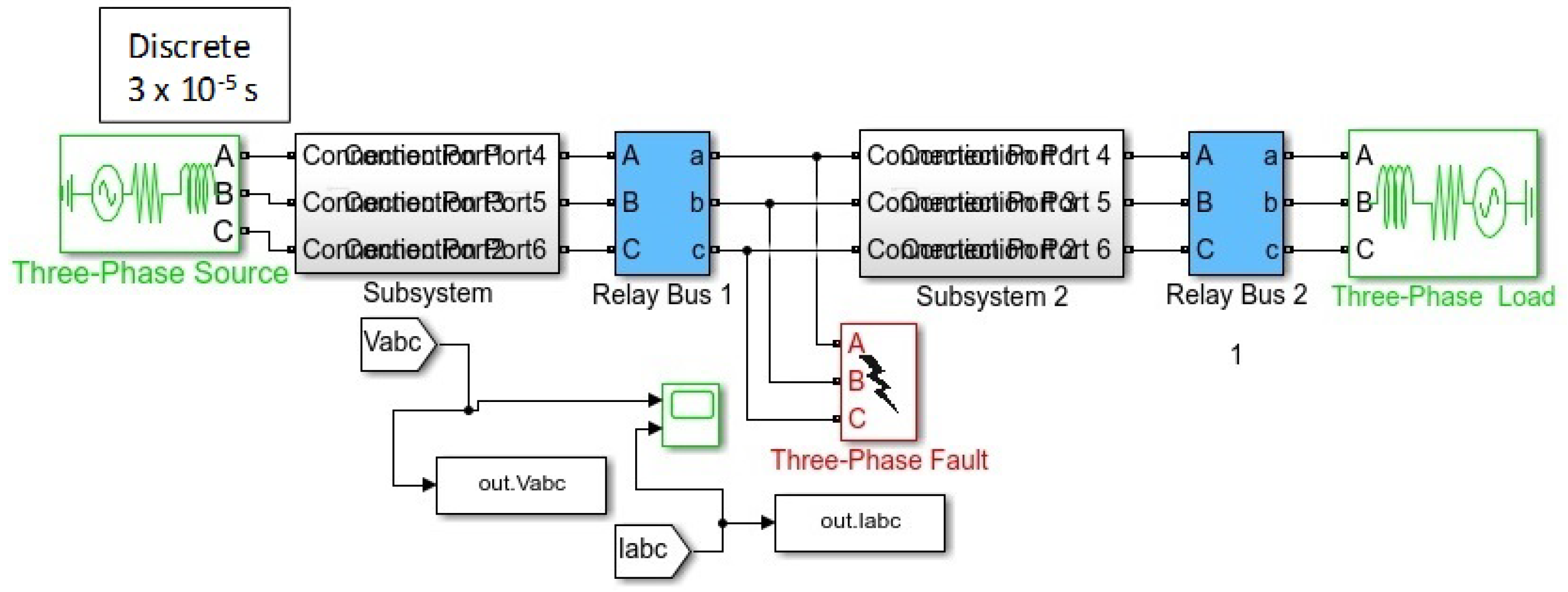
2. Modelling of 330 kV Transmission Line

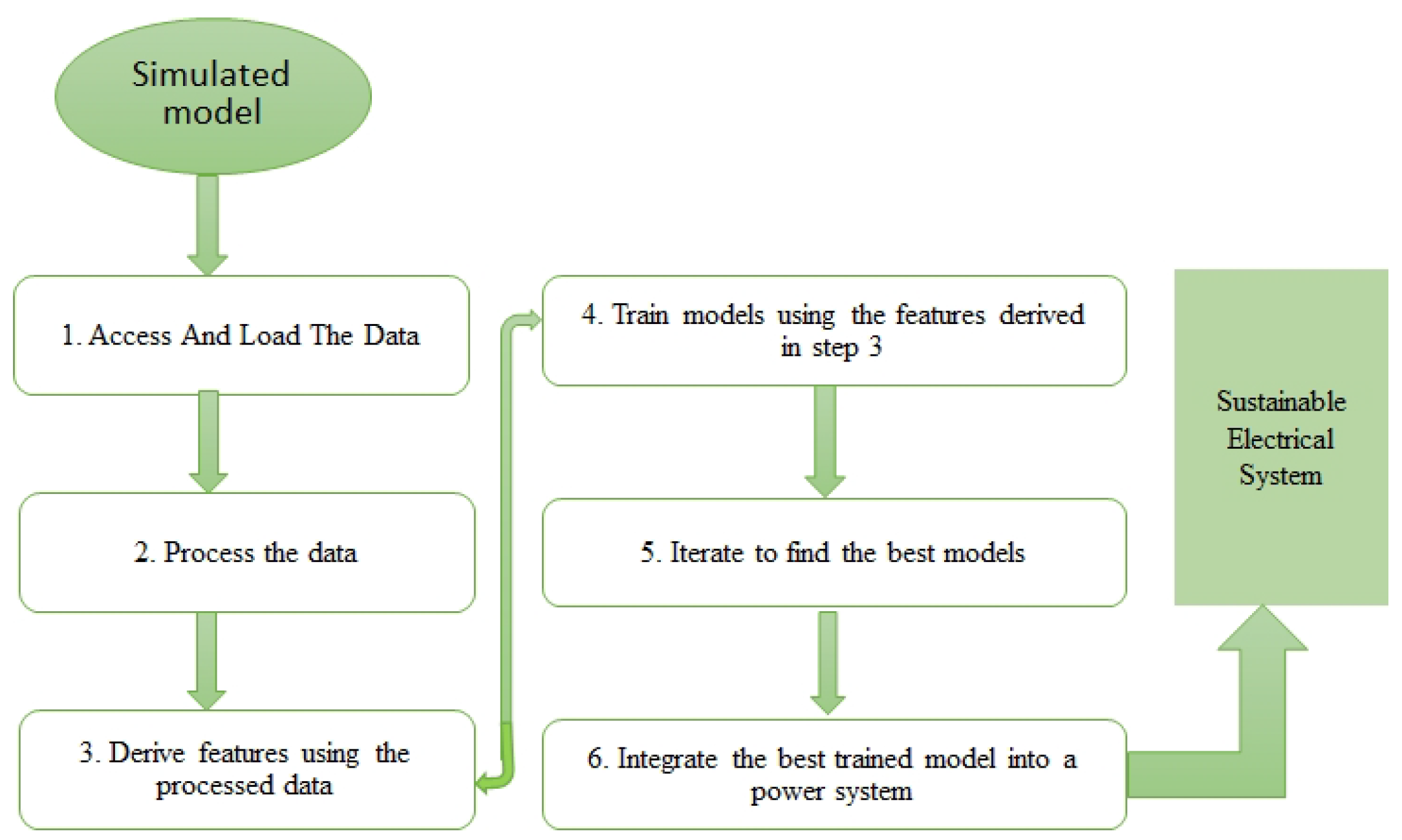
Machine learning needs many datasets for practical training, and those datasets were obtained from a model of a 330 kV, 500 km transmission line network as shown in Figure 1 below. The parameters from

Table 1. Parameters of 330 kV, 500 km transmission line.

Sequence	Parameter	Value	Unit
Positive and negative sequence resistance	$R_1$, $R_2$	0.01273	$\mathsf{\Omega }$/km
Zero sequence resistance	$R_0$	0.3864	$\mathsf{\Omega }$/km
Positive and negative sequence inductance	$L_1$, $L_2$, $L_3$	0.9337 × ${10}^{-3}$	H/km
Zero sequence inductance	$L_0$	4.1264 × ${10}^{-3}$	H/km
Positive and negative sequence capacitance	$C_1$, $C_2$, $C_3$	12.74 × ${10}^{-9}$	F/km
Zero sequence capacitance	$C_0$	7.751 × ${10}^{-9}$	F/km

and

Table 2. Fault parameters of the proposed model.

System Components	Parameters/Units	Value
Phase to phase voltage	voltage	330
Source resistance Rs	Ohms $\left(\mathsf{\Omega }\right)$	0.8929
Source inductance	H	16.58 × ${10}^{-3}$
Fault incipient angle	$\theta$ in degree	0° and −30°
Fault resistance $R_{on}$	Ohms (Ω)	0.001
Ground resistance $R_g$	Ohms (Ω)	0.01
Snubber resistance $R_s$	Ohms (Ω)	1.0 × ${10}^{-6}$
Fault capacitance $C_s$	F	infinite
Switching time	seconds	0.2

were used to create the model in Simulink as in Figure 2. This model generated the fault data of a single line-to-ground, double line-to-ground and three-phase-to-ground fault. These data were used to train machine learning for fault classification. They were also applied to validate the data for accuracy, root mean square error (RMSE) and precision of result.

Figure 1 represents the three-phase, 330 kV transmission line model developed and implemented in this article. It consists of a Nigerian 330 kV transmission line which cut across 500 km and was modelled using Matlab/Simulink. The ground resistance used was 0.01 $\mathsf{\Omega }$ based on the IEEE recommendation for ground resistance, which is ideally in the 0–50 $\mathsf{\Omega }$ range [33]. In addition, a minimum fault line voltage of 0.001 V (minimum standard value) and an incipient fault angle (0 to −30°) were used to derive the maximum arc resistance value. Small ground fault resistance was chosen to detect a transient fault because a higher resistance value would lead to excess voltage and current, so the system might not classify minor faults. Therefore, the higher the fault resistance, the lower the fault detection. A three-phase fault simulator was used to simulate the fault at different locations on the transmission line for proper classification.

Table 1 shows the model parameters where $R_1$ and $R_2$ are positive and negative sequence resistances of phases 1 and 2, respectively. $L_1$, $L_2$ and $L_3$ represent the positive and negative sequence inductances of phases 1, 2 and 3, respectively, whereas $C_1$, $C_2$ and $C_3$ represent the positive and negative sequence voltages of phases 1, 2 and 3, respectively. Finally, $R_0$, $C_0$ and $L_0$ represent the zero resistance, capacitance, and inductance sequence, respectively.

Table 1 and Table 2 represent input data for the modelling of the 330 kV 500 km transmission line. Simulations were carried out by inducing a fault into the line at 300 km. The parameters were carefully selected based on the standard of the International Electro-technical Commission (IEC 60909) [34]. The fault voltage and current data were generated from the model in a different scenario, and 12 fault conditions were considered: are a-g, b-g, c-g, a-b, b-c, a-c, a-b-g, b-c-g, a-c-g, a-b-c, a-b-c-g and no-fault, as seen in

Table 3. Fault types in binary representation.

Class	Fault Type	${\mathit{L}}_1$ (a)	${\mathit{L}}_2$ (b)	${\mathit{L}}_3$ (c)	G (g)
1	a-g	1	0	0	1
2	b-g	0	1	0	1
3	c-g	0	0	1	1
4	a-b	1	1	0	0
5	a-c	1	0	1	0
6	b-c	0	1	1	0
7	a-b-g	1	1	0	1
8	b-c-g	0	1	1	1
9	a-c-g	1	0	1	1
10	a-b-c	1	1	1	0
11	a-b-c-g	1	1	1	1
12	No fault	0	0	0	0

, where a = fault at phase A; b = fault at phase B; c = fault at phase C, and g is the ground fault. The binary representation showed the fault and no-fault conditions representing 1 and 0, respectively. It indicated the fault number assigned to each fault condition.

3. Methodology

It wa possible to achieve fault classification by using phase and zero-sequence current fault data obtained from simulated models. The diagram in Figure 3 shows the data processing model for machine learning used for this article. It involved accessing and loading the data collected from the simulated model into the trainer. Next, the data collected were processed by looking for the data points outside the fitted end of the rest of the data to see if they could be ignored or considered [34].

The next step was to derive features by turning the information into a machine-learning algorithm to improve accuracy, boost model performance, improve model interpretability and prevent overfitting. This was preceded by building and training the model where a confusion matrix was plotted to compare the classification made by design with the actual data collected. Next, we improved the model by checking the correlation matrix to remove variables that were not correlated. The fault data type was introduced in the 500 km, 500 kV transmission line and the dataset was divided into three categories: training, testing, and validation. Each dataset was trained and analysed for final validation, accuracy, errors and performance.

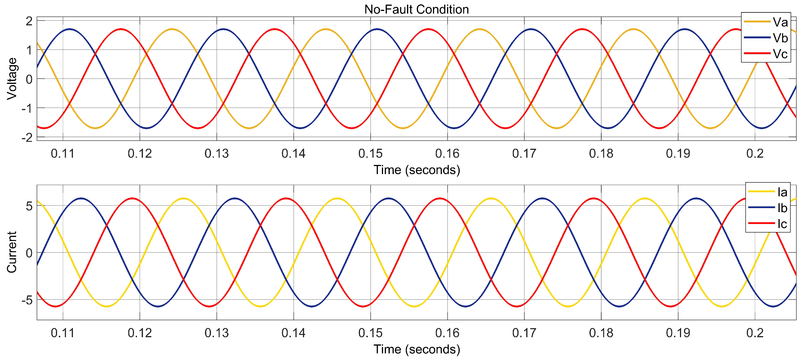
3.1. Data Preparation and Extraction

The faulty data were extracted using the Simulink model from Figure 2, and the waveforms were generated from the model to show the frequency of fault occurrence. The graphs in Figure 4, Figure 5, Figure 6 and Figure 7 show the waveform that validated the presence of a fault in the network. The fault current and voltage were generated and used for machine-language training to classify and locate faults in the transmission line. The waveform displayed in Figure 4 showed standard sinusoidal voltage and current waveforms.

Under the no-fault state, the waveform is sinusoidal and has no distortion due to noise or fault, so the resultant waveform was standard, as seen in Figure 4. When the fault occurred, the fault current of the power transmission line became abnormally high, while the fault voltage decreased to a low value.

Figure 5 shows a three-phase to ground fault where the current and voltage waveform of phase $V_a$, $V_b$, $V_c$ and $I_a$, $I_b$, $I_c$ were distorted by a sudden decrease in their magnitude. In Figure 6 and Figure 7, the voltage and current of phases B, C and A, were also distorted due to faults in the line. All these waveforms showed a distortion due to faults. The switching time of the fault model was set at 0.2 s and the fault location was 250 km along the transmission line. Figure 4, Figure 5, Figure 6 and Figure 7 illustrate fault detection in four different scenarios: no-fault, single-phase-to-ground-fault, double-line-to-ground fault, and three-phase-to-ground fault. The fault current and voltage data were generated, and machine language was used in training the data to detect, classify and locate the fault on the transmission line. The current in Figure 5, Figure 6 and Figure 7 increased drastically, and the voltage fell to zero, as shown in Figure 6, confirming the transmission line fault.

3.2. The Use of CatBoost in Fault Classification

The CatBoost classifier algorithm is used as a machine language tool to train datasets for fault classification to improve its performance, ease of use, and automatic handling of categorical features over other machine language techniques (e.g., the PCA, SVM and ANN). It also requires no explicit pre-processing of data to convert all fault data categories into numbers. A team of engineers from Yandex proposed the model in 2017 [35]. Gradient boosting is a good machine language tool for solving heterogeneous, noisy data and complex variables. It uses binary decision trees as base predictors, and it has the robust characteristics of reducing hyperparameter tuning, and lowering the chances of data overfitting. It combines a gradient boosting decision tree (GBDT) with categorical features, focuses on categorical variables, and deals with gradient bias and prediction shift problems [36]. It helps to improve the robustness of the algorithms by putting all sample datasets into the algorithm for training. When transforming the characteristics of each sample, the target value of the model was calculated before the sample, and the weight and priority were subsequently added. Assuming a data sample size

$$D=\left\{(X_j,Y_i)\right\};j=1,\dots m,$$

(1)

where $X_j=(x_j^1,x_j^2,\dots x_j^n)$ is a vector of n features and response feature $Y_i\in R$, which are binary (1 or 0), and a sample $(X_j,Y_i)$ identically and independently distributed by an unknown distribution $P(.,.)$. The aim is to train a function $H:R^n\to R$ that minimises the expected loss given in Equation (2)

$$L\left(H\right)=EL(y,H(x\left)\right),$$

(2)

where $L(.,.)$ is a smooth loss function and $(X,y)$ is a sample of test data drawn from the training data D [36].

The CatBoost also helps improve the algorithm’s robustness by putting all sample datasets into the algorithm for training. When transforming the characteristics of each sample, the target value of the model is calculated before the sample, and subsequent weight and priority are added. The CatBoost classifier requires minimal data preparation, and it also handles missing values for numerical variables and non-encoded categorical variables. The classification accuracy is used as a criterion to assess the result of fault classification.

3.3. Training of Datasets Using CatBoost Algorithm

About 93,340 datasets of four types of faults, including single-line, double-line to ground, three-phase to ground fault, and no-fault were generated from the Matlab/Simulink fault detection model. The data were divided into training and test datasets of 70% and 30%, respectively. The CatBoost classifier was used as a machine-language tool to train the dataset. The choice of classifier was based on performance and ease of usage. It also had to handle categorical features automatically (without any explicit pre-processing to convert the categories of fault data into numbers), and reduce hyperparameter tuning and the chances of data overfitting. The machine language trainer was simulated with the following parameters:

The input data for the classifier were the fault current and voltage of the transmission line model in Figure 2, and the parameters in

Table 4. CatBoost Classifier training parameter.

CatBoost Model is Fitted	True
Iterations	1000
Depth	10
Loss function	Multiclass
Leaf estimation method	Newton
Class weight	0.001, 0.01, 0.9, 0.001
Random strength	0.1

were used to train the data. The main reason that the CatBoost classifier was preferred is that it is easy to use, efficient, works well with categorical variables, and doesn’t require data pre-processing. It also completed the training in limited time. An effective fault management system requires fast detection and fault classification to protect the power system. This technique is superior to that of other methods, which have longer training times. The parameters were carefully selected through tuning and training to obtain better results and ensure the data was fitted.

4. Results and Discussion

The parameter from

Table 5. Confusion matrix for the fault classification.

True Class	0	0	0	6955	0
	1	0	4862	2051	0
	2	0	0	7048	0
	3	0	0	2013	5073
		0	1	2	3
					Predicted Class

above was used to train the classifier, and the best test accuracy was achieved at 748 iterations out of 1000, which is 99.54% with an error of 0.46%. This result confirmed that the classifier model worked perfectly, and the different types of faults were trained and classified with high accuracy. The no-fault condition was trained separately, and an accuracy of 100% was obtained. This was trained separately to attain a near-perfect classification due to the complexity of the dataset.

Table 6. Fault classification report.

Fault Type	Classes	Precision	Recall	F1-Score	Support
A-G	1	1.00	0.70	0.83	6913
B-C-G	2	0.39	1.00	0.56	7048
A-B-C-G	3	1.00	0.72	0.83	7086
No fault	0	0	0	0	0
	Micro Avg	0.61	0.81	0.69	21,047
	Macro Avg	0.80	0.81	0.74	21,047
	Weighted Avg	0.80	0.81	0.74	21,047

represents the classifier’s confusion matrix, which describes the precision, recall, F1-score, and support. An $N\times N$ matrix was often used to evaluate the performance of the classifier model, where N was the number of target classes. The matrix compared the actual target value with the predicted machine learning model and the error involved. The table shows that the no-fault condition represented 0, the single line to ground fault was 1, the double line to ground was 2, and the three-phase to ground fault was 3. Class 0 was kept at zero because it was at a no-fault condition while the others were trained. The result shows that the model was well fitted, and the four different fault types were well classified.

The accuracy of the model is given as

$$\mathrm{Accuracy}=\frac{TP+TN}{TP+FP+TN+FN}$$

(3)

where $TP$ = True positive; $TN$ = True Negative; $FP$ = False Positive; and $FN$ = False Negative. Furthermore,

$$\mathrm{Precision}=\frac{TP}{TP+FP}.$$

(4)

tells how many of the predicted cases turned out to be positive, and determines whether the model was reliable. In Table 6, the precision in single-phase to ground and three-phase fault was 1, which showed that the model was worked perfectly well. ‘Recall’ shows how many of the actual positive cases were predicted correctly and is given by

$$\mathrm{Recall}=\frac{TP}{TP+FN}.$$

(5)

The double line to ground fault was predicted correctly compared to other faults, as shown in Table 6. Also, the F1-Score was the harmonic mean of precision and recall and is given by:

$$\mathrm{F}1-\mathrm{Score}=\frac{2}{\frac{1}{\mathrm{Recall}}+\frac{1}{\mathrm{Precision}}}$$

(6)

True-positive indicated that the classifier predicted a true event, and the event was true, whereas true-negative indicates that the classifier predicted a false event, and the event was false. The false positive classifier predicted that an event would occur, but it was incorrect. Still, the event was not true, whereas the false-negative indicated that the event was incorrectly predicted and was therefore false. The results from the fault classification report in Table 6 also affirmed that the classifier produced perfect results. Therefore, it was a better classifier for training multi-datasets than were those from the reviewed literature.

Table 7. Comparing different machine learning techniques for accuracy in fault classification.

Technique Used	Input Parameter	Fault Types	Data Size	% Accuracy	Strength	Weakness
WT, CNN [20]	vibration signal	400 different fault condition	2400	97.78%	speed of 8 s to execute and easy to use	The WT Packet is not theoretically proven.
ANN [37]	Three-phase voltage and current waveform	10 different fault condition	7920	78.1%	Easy to use and implement, Repro- gramming is not needed	Requires a system with a high processor, Longer training time.
Proposed CatBoost Classifier	Voltage and current signal	Single-phase fault, double phase fault, three-phase fault and no-fault	93,340 X 6	99.54%	Higher accuracy, speed and low training time.multiple feature classification	It needs a high- performance operating system to train the data.
BPNN [11]	Voltage and current	AG, BG, CG, ABG, ACG, BCG, AB, AC, BC, ABC, ABCG	1188	97.3%	easy to execute, it requires less number of neurons for training.	Slow to use, computationally expensive, can’t be used to solve complex andlarge problems. Slow convergence.
RBFNN [11]	Voltage and current	AG, BG, CG, ABG, ACG, BCG, AB, AC, BC, ABC, ABCG	1188	99.3%	Faster than BPNN, easy to use.	Not suitable for non-linear systems and large dataset
PNN [11]	Voltage and current	AG, BG, CG, ABG, ACG, BCG, AB, AC, BC, ABC, ABCG	1188	99.4%	It can handle multi-dataset to classify faults. Also, no learning process is required.	Expensive to implement, and learning can be slow, high processing time if the network is extensive.
RDRP [19]	Voltage signal of 10 dB, 20 dB and 30 dB	Single, double and three-phase fault	480	93.9, 96.8% and 96.8%	It can work well with small datasets	Not suitable for multiple datasets and low prediction accuracy.
CNN [16]	Three phase Voltage and current	10 different fault condition	92,077	99%	Used to solve multi-channel sequence recognition problem	The computational cost of offline mode is expensive

compares the different machine-learning techniques used in fault classification based on various methods and justifies the use of the algorithm, focusing on accuracy, speed, and strength. The CatBoost classifier produced a better result than did the other classifiers, as seen in Table 7, with an accuracy of 99.54%. The CatBoost technique was chosen over other methods for its speed, accuracy and low training time for classifying faults according to different categories. It can also accurately handle multi-datasets of different fault currents and voltage at the same time.

5. Discussion

The CatBoost classifier produced exceptional results because its accuracy and precision were better than the other methods used in the literature. In another research study, the use of sparse representation classification with random dimensionality reduction projection technique was used to classify faults [38]. This method generated results ranging from 93.9%, 96.8% and 98.8% for 10 dB, 20 dB and 30 dB, respectively, which varied according to fault type [19]. In [14], S-transform and neural networks were used in fault classification, and the average accuracy was 99.6%. Still, the research of [14] was based on a three-phase fault in contrast to the four fault types used in this paper. The recursive neural network (RNN) was used in [19], and about 500 pieces of fault data were used, but the classifier failed to classify L-L and L-L-G fault types at 140 km. However, it was able to classify the fault in some distance with an accuracy of 98.67%, so the classifier’s inability to classify all the different types of faults at different locations made it unsuitable as a fault classification technique. The CatBoost algorithm was proven to be a better machine learning tool in fault classification and detection for the training of data and is highly recommended for optimum, accurate results.

Figure 8 shows a separate analysis of the performance of the CatBoost model where the single-phase and three-phase fault performs optimally with accuracy of 100% while the recall value was higher for the double phase-to-ground fault.

The novelty of this paper is the use of the CatBoost classifier for transmission line fault classification. Table 7 enumerates some of its distinctive features over other machine-learning algorithms, including an overall result accuracy of 99.54% and an individual line fault accuracy of 100% in a three-face fault classification. The execution speed 58.5 s compared with that of the SVM. The model also handled a multi-dataset, combined multiple categorical features, and overcame gradient bias. It also prevented data overfitting and data pre-processing during training compared to techniques that use trial and error for parameter tuning, in contrast to other machine learning algorithms like SVM, K-NN, CNN and RNN.

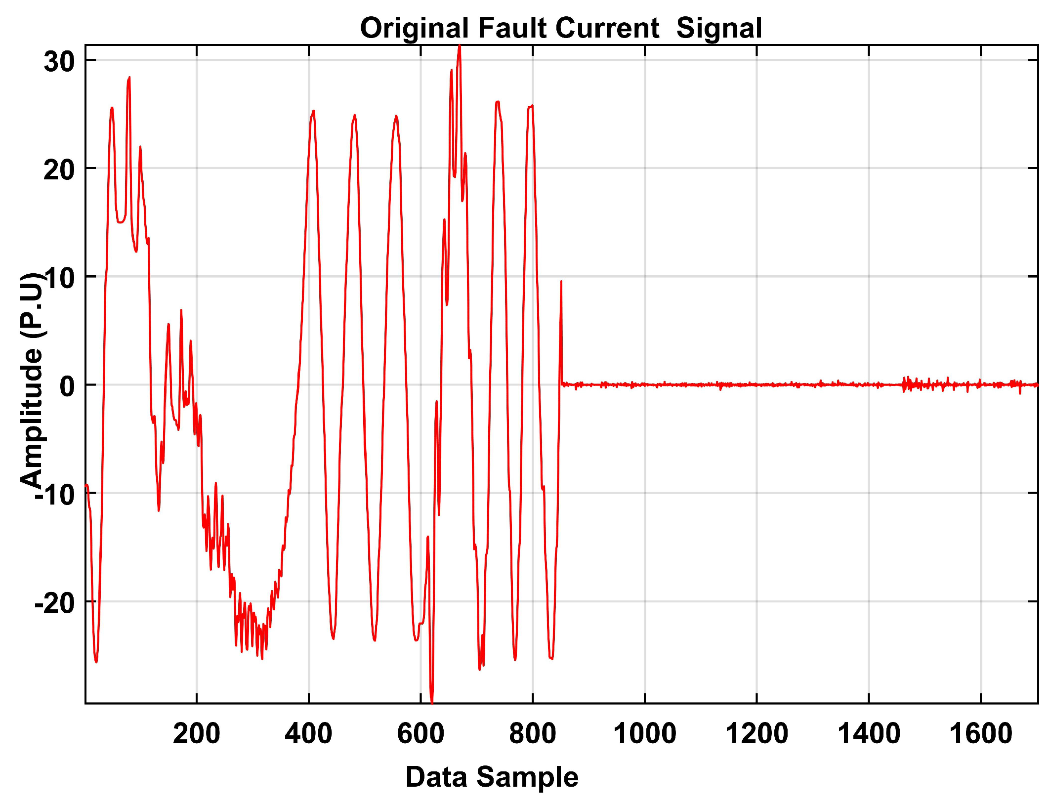
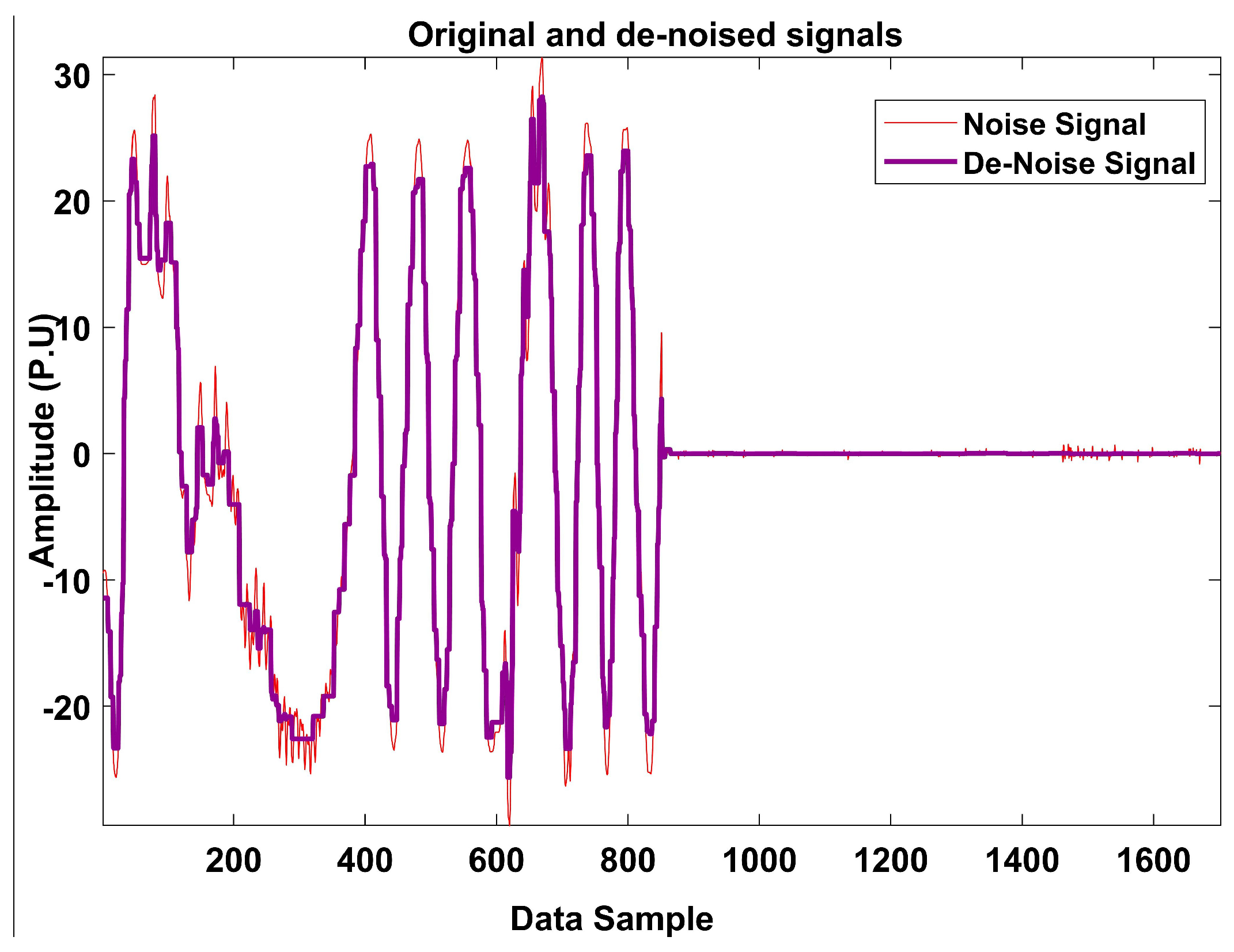
The Effect of Noise and Disturbance in the Proposed Algorithm

Power quality disturbance (PQDs) and noise signals have adverse effects on fault classification in transmission line accuracy. During feature selection and extraction, it is necessary to consider noise and signal disturbance because of voltage swell, sag, interruption and flicker; transient oscillation; harmonics; and transient impulses. In the proposed model, noise signals and PQDs were considered and compared with other articles, and it was observed that the CatBoost classifier performed better, with accuracy remaining at 99.54% both in noise and noiseless signals. This showed that the method effectively reduced the effects of noise and disturbance on classification accuracy. In [39], the ANN technique was used for classification with a noiseless signal accuracy of 87.55% and 82.44% at 20 dB noise. In [40], the DWT was used for feature extraction, and the SVM was used for fault classification with an accuracy of 100% without disturbance and 98 and 95.6% accuracy at 30 and 20 dB noise, respectively.

The novelty of the proposed method is the ability of the model to “de-noise” the signal for optimal performance, as seen in Figure 9 and Figure 10. The current signal in the three phase-to-ground faults was de-noised for optimal model performance before it was integrated into the CatBoost classifier. In Figure 9 the base current rose to 30 per unit (PU) which caused a disturbance in the system but was reduced to 28 PU as seen in Figure 10. The process can continue to achieve a zero signal to noise ratio in the system.

In addition, the power quality can be improved by this method for quality control, and online and offline fault classification with noise and noiseless data. This can be applied in fault management and protection in high-voltage transmission lines, and the distribution network and technique can help in fault management and protection when noise and disturbances are inevitably present.

6. Conclusions

Faults affect the transmission line and cause significant damage to equipment and power disruptions to the customers or end-users. These faults occur due to bad weather conditions or faulty equipment, and transient faults are the result of human interference. Hence, there is need to model a system that will classify, detect and isolate faults accurately within the shortest time of detection.

This paper proposed the use of the CatBoost classifier as the preferred algorithm for fault classification because of its high accuracy and ease of training. This technique is achieved first by designing a 330 kV, 500 km transmission line using Matlab/Simulink to extract the fault current and voltage to identify the fault phase for each faulty voltage and current waveform. A 93,340 fault dataset was used to train the algorithm, and the result provided a better accuracy of 99.54%. The classifier algorithms are capable of training multi-dataset categorical data such as the SVM, ANN and XBoost classifiers.

This paper addressed the classification of a multi-dataset of faulty voltage and current in transmission lines focusing on speed, accuracy and precision for fast detection and isolation of faults. The results also served as a guide on transmission line fault protection management systems and design. The CatBoost classifier was justified for the transmission line fault classification model after being compared to other methods in other literature. This paper can be improved by varying the fault resistance to different values from 0.01 to 50 Ω and beyond. The model can also be optimised for real time data mining and automatic training for an effective fault protection mechanism.

References

1. Singh, M.R.; Chopra, T.; Singh, R.; Chopra, T. Fault classification in electric power transmission lines using support vector machine. Int. J. Innov. Res. Sci. Technol. 2015, 1, 388–400. [Google Scholar]
2. Chang, G.W.; Hong, Y.H.; Li, G.Y. A hybrid intelligent approach for classification of incipient faults in transmission network. IEEE Trans. Power Deliv. 2019, 34, 1785–1794. [Google Scholar] [CrossRef]
3. Rahmati, A.; Adhami, R. A fault detection and classification technique based on sequential components. IEEE Trans. Ind. Appl. 2014, 50, 4202–4209. [Google Scholar] [CrossRef]
4. Chen, K.; Huang, C.; He, J. Fault detection, classification and location for transmission lines and distribution systems: A review on the methods. High Volt. 2016, 1, 25–33. [Google Scholar] [CrossRef]
5. Swetapadma, A.; Yadav, A. An artificial neural network-based solution to locate the multilocation faults in double circuit series capacitor compensated transmission lines. Int. Trans. Electr. Energy Syst. 2018, 28, e2517. [Google Scholar] [CrossRef]
6. Uzubi, U.; Ekwue, A.; Ejiogu, E. Artificial neural network technique for transmission line protection on Nigerian power system. In Proceedings of the 2017 IEEE PES PowerAfrica, Accra, Ghana, 27–30 June 2017; pp. 52–58. [Google Scholar]
7. Dos Santos, R.C.; Senger, E.C. Transmission lines distance protection using artificial neural networks. Int. J. Electr. Power Energy Syst. 2011, 33, 721–730. [Google Scholar] [CrossRef]
8. Prasad, A.; Edward, J.B. Importance of artificial neural networks for location of faults in transmission systems: A survey. In Proceedings of the 2017 11th International Conference on Intelligent Systems and Control (ISCO), Coimbatore, India, 5–6 January 2017; pp. 357–362. [Google Scholar]
9. Manke, P.R.; Tembhurne, S. Artificial neural network classification of power quality disturbances using time-frequency plane in industries. In Proceedings of the 2008 First International Conference on Emerging Trends in Engineering and Technology, Nagpur, India, 16–18 July 2008; pp. 564–568. [Google Scholar]
10. Reddy, M.J.B.; Gopakumar, P.; Mohanta, D. A novel transmission line protection using DOST and SVM. Eng. Sci. Technol. Int. J. 2016, 19, 1027–1039. [Google Scholar]
11. Alsubhi, S.R.; Laabidi, K.; Hsairi, L. Comparison of Several Artificial Neural Network Approaches for Fault Classification in Power Transmission Lines. In Proceedings of the 7th International Conference on Engineering & MIS 2021, Almaty, Kazakhstan, 11–13 October 2021; pp. 1–6. [Google Scholar]
12. Abdulwahid, A.H. A new concept of an intelligent protection system based on a discrete wavelet transform and neural network method for smart grids. In Proceedings of the 2019 2nd International Conference of the IEEE Nigeria Computer Chapter (NigeriaComputConf), Zaria, Nigeria, 14–17 October 2019; pp. 1–6. [Google Scholar]
13. Costa, F.B.; Silva, K.M.; Souza, B.A.; Dantas, K.M.C.; Brito, N.S.D. A method for fault classification in transmission lines based on ann and wavelet coefficients energy. In Proceedings of the The 2006 IEEE International Joint Conference on Neural Network Proceedings, Vancouver, BC, Canada, 16–21 July 2006; pp. 3700–3705. [Google Scholar]
14. Roy, N.; Bhattacharya, K. Detection, classification, and estimation of fault location on an overhead transmission line using S-transform and neural network. Electr. Power Compon. Syst. 2015, 43, 461–472. [Google Scholar] [CrossRef]
15. Rai, P.; Londhe, N.D.; Raj, R. Fault classification in power system distribution network integrated with distributed generators using CNN. Electr. Power Syst. Res. 2021, 192, 106914. [Google Scholar] [CrossRef]
16. Chopra, P.; Yadav, S.K. PCA and feature correlation for fault detection and classification. In Proceedings of the 2015 IEEE Recent Advances in Intelligent Computational Systems (RAICS), Trivandrum, India, 10–12 December 2015; pp. 195–200. [Google Scholar]
17. Ni, J.; Zhang, C.; Yang, S.X. An adaptive approach based on KPCA and SVM for real-time fault diagnosis of HVCBs. IEEE Trans. Power Deliv. 2011, 26, 1960–1971. [Google Scholar] [CrossRef]
18. Wang, Q.; Wei, B.; Liu, J.; Ma, W. Data-Driven Incipient Fault Prediction for Non-Stationary and Non-Linear Rotating Systems: Methodology, Model Construction and Application. IEEE Access 2020, 8, 197134–197146. [Google Scholar] [CrossRef]
19. Cheng, L.; Wang, L.; Gao, F. Power system fault classification method based on sparse representation and random dimensionality reduction projection. In Proceedings of the 2015 IEEE Power & Energy Society General Meeting, Denver, CO, USA, 26–30 July 2015; pp. 1–5. [Google Scholar]
20. Zhao, M.; Fu, X.; Zhang, Y.; Meng, L.; Tang, B. Highly imbalanced fault diagnosis of mechanical systems based on wavelet packet distortion and convolutional neural networks. Adv. Eng. Inform. 2022, 51, 101535. [Google Scholar] [CrossRef]
21. Zhao, X.; Yao, J.; Deng, W.; Ding, P.; Ding, Y.; Jia, M.; Liu, Z. Intelligent Fault Diagnosis of Gearbox Under Variable Working Conditions With Adaptive Intraclass and Interclass Convolutional Neural Network. IEEE Trans. Neural Netw. Learn. Syst. 2022, 1–15. [Google Scholar] [CrossRef] [PubMed]
22. Zhao, X.; Yao, J.; Deng, W.; Jia, M.; Liu, Z. Normalized Conditional Variational Auto-Encoder with adaptive Focal loss for imbalanced fault diagnosis of Bearing-Rotor system. Mech. Syst. Signal Process. 2022, 170, 108826. [Google Scholar] [CrossRef]
23. Moradzadeh, A.; Teimourzadeh, H.; Mohammadi-Ivatloo, B.; Pourhossein, K. Hybrid CNN-LSTM approaches for identification of type and locations of transmission line faults. Int. J. Electr. Power Energy Syst. 2022, 135, 107563. [Google Scholar] [CrossRef]
24. Mishra, D.P.; Samantaray, S.R.; Joos, G. A combined wavelet and data-mining based intelligent protection scheme for microgrid. IEEE Trans. Smart Grid 2015, 7, 2295–2304. [Google Scholar] [CrossRef]
25. Ogar, V.N.; Gamage, K.A.; Hussain, S. Protection for 330 kV transmission line and recommendation for Nigerian transmission system: A review. Int. J. Electr. Comput. Eng. 2022, 12, 3320–3334. [Google Scholar] [CrossRef]
26. Kar, S.; Samantaray, S.R. Time-frequency transform-based differential scheme for microgrid protection. IET Gener. Transm. Distrib. 2014, 8, 310–320. [Google Scholar] [CrossRef]
27. Roy, N.; Bhattacharya, K. Identification and classification of fault using S-transform in an unbalanced network. In Proceedings of the 2013 IEEE 1st International Conference on Condition Assessment Techniques in Electrical Systems (CATCON), Kolkata, India, 6–8 December 2013; pp. 111–115. [Google Scholar]
28. Raza, A.; Benrabah, A.; Alquthami, T.; Akmal, M. A review of fault diagnosing methods in power transmission systems. Appl. Sci. 2020, 10, 1312. [Google Scholar] [CrossRef] [Green Version]
29. Mukherjee, A.; Kundu, P.K.; Das, A. A supervised principal component analysis-based approach of fault localization in transmission lines for single line to ground faults. Electr. Eng. 2021, 103, 2113–2126. [Google Scholar] [CrossRef]
30. Elnozahy, A.; Sayed, K.; Bahyeldin, M. Artificial neural network based fault classification and location for transmission lines. In Proceedings of the 2019 IEEE Conference on Power Electronics and Renewable Energy (CPERE), Aswan, Egypt, 23–25 October 2019; pp. 140–144. [Google Scholar]
31. Al-Shaibani, S.A.; Bhalchandra, P. A Framework for Implementing Prediction Algorithm over Cloud Data as a Procedure for Cloud Data Mining. J. Electr. Electron. Eng. 2021, 2, 1–8. [Google Scholar] [CrossRef]
32. Godse, R.; Bhat, S. Mathematical morphology-based feature-extraction technique for detection and classification of faults on power transmission line. IEEE Access 2020, 8, 38459–38471. [Google Scholar] [CrossRef]
33. De Andrade, V.; Sorrentino, E. Typical expected values of the fault resistance in power systems. In Proceedings of the 2010 IEEE/PES Transmission and Distribution Conference and Exposition: Latin America (T&D-LA), Sao Paulo, Brazil, 8–10 November 2010; pp. 602–609. [Google Scholar]
34. Sweeting, D. Applying IEC 60909, fault current calculations. IEEE Trans. Ind. Appl. 2011, 48, 575–580. [Google Scholar] [CrossRef]
35. Prokhorenkova, L.; Gusev, G.; Vorobev, A.; Dorogush, A.V.; Gulin, A. CatBoost: Unbiased boosting with categorical features. Adv. Neural Inf. Process. Syst. 2018, 31. [Google Scholar]
36. Zhang, Y.; Zhao, Z.; Zheng, J. CatBoost: A new approach for estimating daily reference crop evapotranspiration in arid and semi-arid regions of Northern China. J. Hydrol. 2020, 588, 125087. [Google Scholar] [CrossRef]
37. Jamil, M.; Sharma, S.K.; Singh, R. Fault detection and classification in electrical power transmission system using artificial neural network. SpringerPlus 2015, 4, 1–13. [Google Scholar] [CrossRef] [PubMed] [Green Version]
38. Ibrahim, A.A.; Ridwan, R.L.; Muhamme, M.; Abdulaziz, R.O.; Saheed, G.A. Comparison of the CatBoost classifier with other machine learning methods. Int. J. Adv. Comput. Sci. Appl. 2020, 11, 738–748. [Google Scholar] [CrossRef]
39. Mishra, M. Power quality disturbance detection and classification using signal processing and soft computing techniques: A comprehensive review. Int. Trans. Electr. Energy Syst. 2019, 29, e12008. [Google Scholar] [CrossRef] [Green Version]
40. Erişti, H.; Uçar, A.; Demir, Y. Wavelet-based feature extraction and selection for classification of power system disturbances using support vector machines. Electr. Power Syst. Res. 2010, 80, 743–752. [Google Scholar] [CrossRef]
Figure 1. A 330 kV three-phase, 500 km transmission line model.
Signals 03 00027 g001
Figure 2. Simulink Model of 330 kV. 500 km transmission line.
Signals 03 00027 g002
Figure 3. The data processing model for machine learning.
Signals 03 00027 g003
Figure 4. Three -phase at no fault condition.
Signals 03 00027 g004
Figure 5. Three-phase to ground fault (a-b-c-g).
Signals 03 00027 g005
Figure 6. Double-phase to ground fault (a-b-g).
Signals 03 00027 g006
Figure 7. Single-phase to ground fault (a-g).
Signals 03 00027 g007
Figure 8. Performance of the different faults types.
Signals 03 00027 g008
Figure 9. Fault Current with Noise Signal.
Signals 03 00027 g009
Figure 10. Fault Current With De-Noise Signal.
Signals 03 00027 g010