Sound Scattering by Gothic Piers and Columns of the Cathédrale Notre-Dame de Paris

Abstract

Although the acoustics of Gothic cathedrals are of interest to researchers, the acoustic impact of their many columns is often neglected. The construction of the Cathédrale Notre-Dame de Paris spanned several centuries, including a wide variety of architectonic elements. This study investigates the sound scattering of a selection of seven designs that are relevant to this building as well as to the architectural style itself. These were measured on scale models (1:8.5 to 1:12), using a subtraction method, for receivers at about 3 m at full scale and a far-field source. They were also numerically simulated using a finite-difference time-domain method in two-dimensional space with an incident plane wave. The method integrates a finite volume framework to employ an unstructured mesh conforming to the complex geometries of interest. The two methods are in strong agreement for the considered configurations. Relative levels to the direct sound of backscattered reflections between $-10$ dB and 2 dB and between $-15$ dB and $-6$ dB in the transverse directions were estimated for the dimensions considered, relative to reported reflection audibility thresholds. Cross-sections with smaller scale geometrical elements on their perimeter can produce diffuse reflections similar to those of surface diffusers.

1. Introduction

In large ancient buildings such as Gothic churches and cathedrals, columns and piers (In art history, a column refers to a support based on a circular section, while a pier is a generic term.) with different shapes can be present in a large number. These architectonic elements are obstacles that can scatter a wave in all directions when it reaches it. In this case, the term volumetric diffuser has been proposed [1]. Examples of modern applications are the canopy of reflectors suspended above some concert hall stages [2] or hanging panels in reverberation chambers [3]. As they are finite-sized objects, they usually have less effect on long wavelengths [4], and the effect of the curvature of reflector panels on this frequency limit has been considered [5,6]. For wavelengths of comparable size, the waves can propagate around the obstacle and are strongly diffracted, notably in the shadow zone [7]. The rows of columns surrounding the nave in a church, delimiting the subspaces, can be seen as lateral reflectors. In the Cathédrale Notre-Dame de Paris, cylindrical obstacles are found with cross-sectional shapes that are representative of different Gothic styles as its construction spanned several centuries. Among them, some are concave, star-shaped or not, involving intersecting circles, and outer and inner corners that in the end, form grooves and cavities; others are formed with multiple cylinders. The present study aims to examine the scattered reflections of different selected geometries that are relevant regarding the origin and the evolution of Gothic architecture, through numerical simulations and physical scale model measurements.

In room acoustics, studies concerning scattered reflections have often been interested in that of wall surfaces whose properties can be characterized in the far field using standardized procedures to determine the scattering [8] and diffusion [9] coefficients. Their effects on the sound field of concert halls have been evaluated perceptually and objectively by examining the room acoustic parameters with scale [10,11,12] and computer [11,13,14] models. Similarly, the effect of circular columns placed close to the walls of a concert hall has been studied in [15]. In contrast, we propose here to study the reflections of obstacles in isolation, similarly to [6], with a far-field source and a receiver at distances representative of a listening situation in the cathedral.

Wave scattering by cylindrical objects has been of interest for a long time, and different methods have been applied to address different geometries, boundary conditions, and frequency ranges. Lord Rayleigh was the first to derive wave scattering by small obstacles compared to the wavelength [16]. Subsequently, analytical solutions using partial wave series expansion methods have been derived for simple shapes [17,18]. The study of more arbitrary geometries involving complex shapes and/or multiples bodies can be achieved using measurements on full-size [5] or scale models [19] and simulations with appropriate computational methods. Frequency methods solving the Helmholtz equation, such as the boundary element method [20,21] or the finite element method [22] have been employed. Time domain methods solving the wave equation allow for the study of scattering on a wide frequency band through the use of pulse excitation and to evaluate the temporal spreading occurring. They are widely used in the field of electromagnetism for the study of antennas [23]. In the field of acoustics, they have been applied to the characterization of sound diffusers [24] and sonic crystals [25,26]. Nevertheless, they suffer from numerical dispersion causing the anisotropy of phase velocities in the discrete space [23]. Moreover, if the boundaries of the scattering object are meshed from a regular grid, which in most cases does not conform to it, staircasing artifacts appear [27]. In this work, a finite difference scheme solving the two-dimensional wave equation by operating on a hexagonal grid is used in conjunction with a finite volume method operating on an unstructured mesh in proximity to the boundaries [28]. These artifacts are thus eliminated, the isotropy is improved, and the dispersion is reduced compared to other compact Cartesian schemes [29].

The audibility of early reflections is usually expressed in terms of detection threshold or masked threshold, defined as the highest level of a reflection just before it becomes inaudible, relative to the direct sound [30]. This depends on many factors, including the delay of the reflection, its direction, the signal type, its spectrum and its sound level, or the environment. Their influence has been addressed in several studies [30,31,32,33,34,35,36,37]. A practical “rule of thumb” has been proposed [35], such that early reflections will be inaudible if their levels are less than −22 dB relative to the direct sound for a 3 ms delay, lowered to −31 dB for 15 ms to 30 ms, and that a modest amount of reverberation added in the stimuli increases the thresholds by up to 11 dB. This criterion has been adapted to discuss the audibility of reflections from panels with various curved edges [6]. These thresholds are also related to the human ability to echolocate dicrete objects [38,39]. The effect of diffusion has been studied by Robinson et al. [40]. White Gaussian noise was multiplied with gamma distributions of different parameters to emulate the temporal spreading and envelope of diffuse reflections. In comparison to specular reflections with the same peak amplitude, diffuse reflections were more detectable, indicating that integrated power of the reflection is probably a better indicator to predict its audibility. Wendt and Höldrich [41] considered reflections from a finite wall modeled with Lambertian surface. They found similar results that they attributed to the temporal position of the energy centroid for a diffuse reflection in relation to the forward masking pattern of the direct sound. In addition, they provide relationships linking the masking thresholds to the logarithm of the time differences of arrival, with excellent correlations to the experiments. Our ability to perceptually discriminate between different reflections from surfaces with respect to their topology inducing spectral coloration has been studied in [42], and with finite-difference time-domain method simulations in [43,44].

A brief introduction reviewing the long construction of Notre-Dame de Paris and its acoustics is given first in Section 1.1 and Section 1.2, and the cross-sections of the columns and piers studied are then described in Section 2.1. The numerical methods and set-ups used are presented in Section 2.2. Sound scattering is additionally measured on 1:8.5 to 1:12 scale models of the selected piers and columns. The protocol and post-processing methods used to isolate the scattered pressure are described in Section 2.3. Measurements and simulations are compared for cross-validation in Section 3.1 and Section 3.2. Simulation results are analyzed in the time-frequency domain and presented in a perceptually relevant way in Section 3.3 Finally, we discuss their efficiency in terms of volumetric diffusers and their audibility with respect to the thresholds reported in the literature in Section 4.

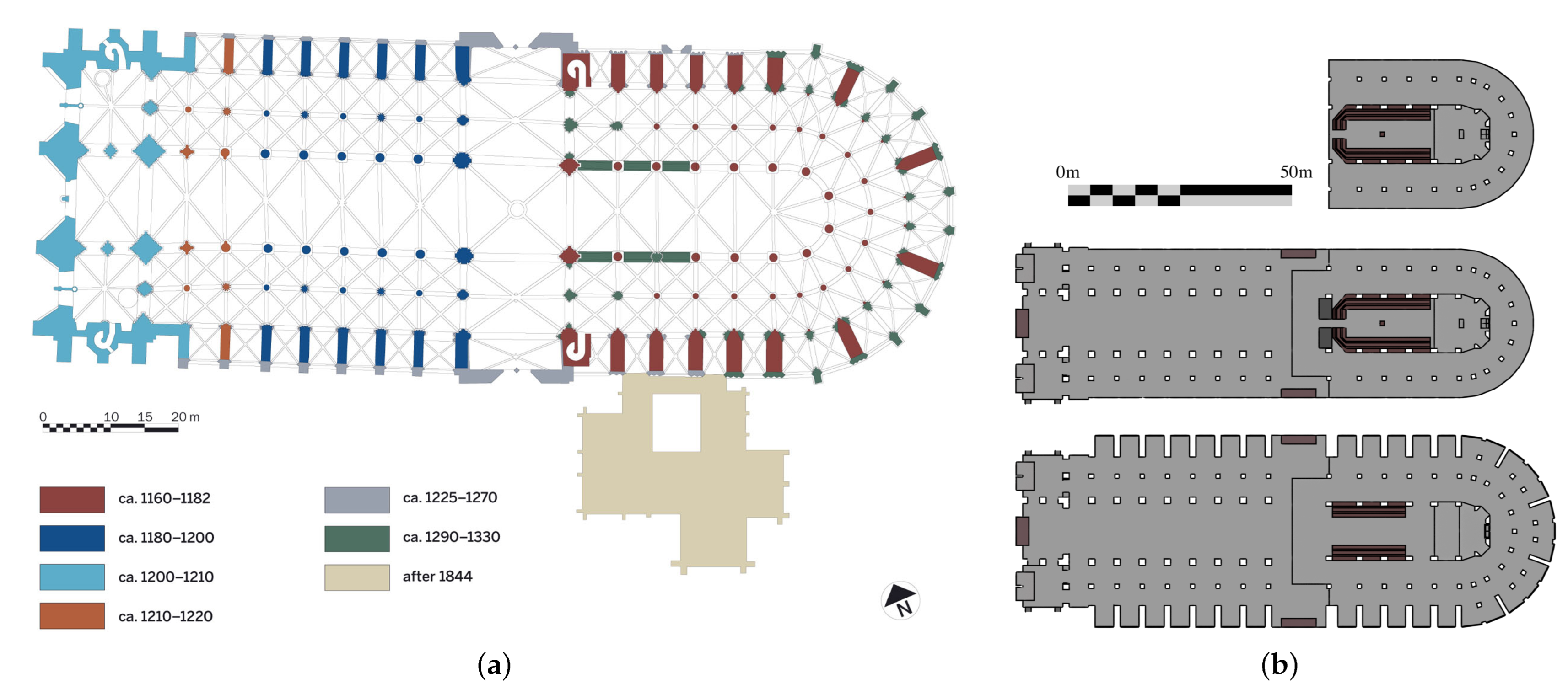
1.1. Introduction to the History of the Construction of Notre-Dame de Paris

The history of the construction of Notre-Dame de Paris has been treated in detail by several authors [45,46,47,48]. We recall here the main stages of it, as well as some background information.

The construction of the Cathédrale Notre-Dame de Paris began in 1163 under the responsibility of Maurice de Sully, bishop of Paris. Figure 1a shows the principal phases of construction. The first part to be built was the choir, completed in 1182, as shown at the top of Figure 1b. At this date, the western wall of the transept was already erected. The choir had a double ambulatory and tribunes as with nowadays, but did not have its radiating chapels yet. The elevation of the nave started in 1180 while the vaults were missing in the choir. Several construction campaigns will have been necessary for the western part of the cathedral to be completed. The first bay of the nave, connecting it to the facade composed of the bases of the towers, was completed around 1220. While the construction of the towers continued, changes were made to the building from 1225, following a fire between the roof and the vaults according to Viollet-le-Duc [47]. At that time, the work had already been going on for more than 60 years, a period during which the techniques of masonry knew many innovations. Thus, the hypothesis that, by rivalry with other dioceses building cathedrals at the same time, the bishop would have decided to bring it up-to-date has also been advanced [47]. The towers were completed around 1240, at the same time that the lateral chapels were added to the nave. Around 1250, the rose window of the north arm of the transept, extended by one bay, was built by the master mason Jean de Chelles and that of the south, added 10 years latter, is attributed to his successor, Pierre de Montreuil. In the meantime, a wooden spire was added above the crossing. The radiating chapels were built between 1290 and 1330 under the supervision of Pierre de Chelles and his successor, Jean Ravy.

It took almost two centuries for the cathedral to reach a shape close to the one we know today, and it is only from the 18th century that major modifications were made to the interior. After the Vow of Louis XIII in 1638, the cathedral underwent a period sometimes qualified as a Baroque transformation, with the addition of the still present polychromatic marble pavement, Pietà, and oak stalls. After the French Revolution, the building was requisitioned and rededicated as the Temple of Reason on 10 November 1793. It returned to the clergy less than 10 years later, on 10 April 1802, in a more deteriorated state than it already was. In 1843, Lassus and Viollet-le-Duc won the tender for a renovation project [50], being the only ones to submit on time. Their wish was to return to a state closer to the cathedral’s origins. They removed some of the additions from the Baroque period but renovated some of them, such as the pavement. They rebuilt a spire above the crossing in imitation of the 13th century one that had to be dismantled at the end of the 18th century because it showed signs of fragility and was in danger of collapsing. Oculi were introduced at the level of the triforium (Triforium: Narrow level below the clerestory. ) on the walls of the transept, on the last bay of the nave and the first of the choir. These renovations, lasting for almost 20 years, were conscientiously consigned in a daily work journal [51].

1.2. General Acoustics of Notre-Dame de Paris

The Cathedral suffered a major fire in April 2019. However, measurements were taken almost 4 years earlier [52]. The reverberation time $T_{20}$ measured at that time was about 7 s at 500 Hz. Additional measurements were subsequently made by the authors after the fire in 2020 [53]. Among the damages, several vaults collapsed, including the one at the crossing, created large openings. The reduction in reverberation time was estimated to be 8% on average. More information on the acoustics in past states, obtained by simulations, is available in [49].

2. Materials and Methods

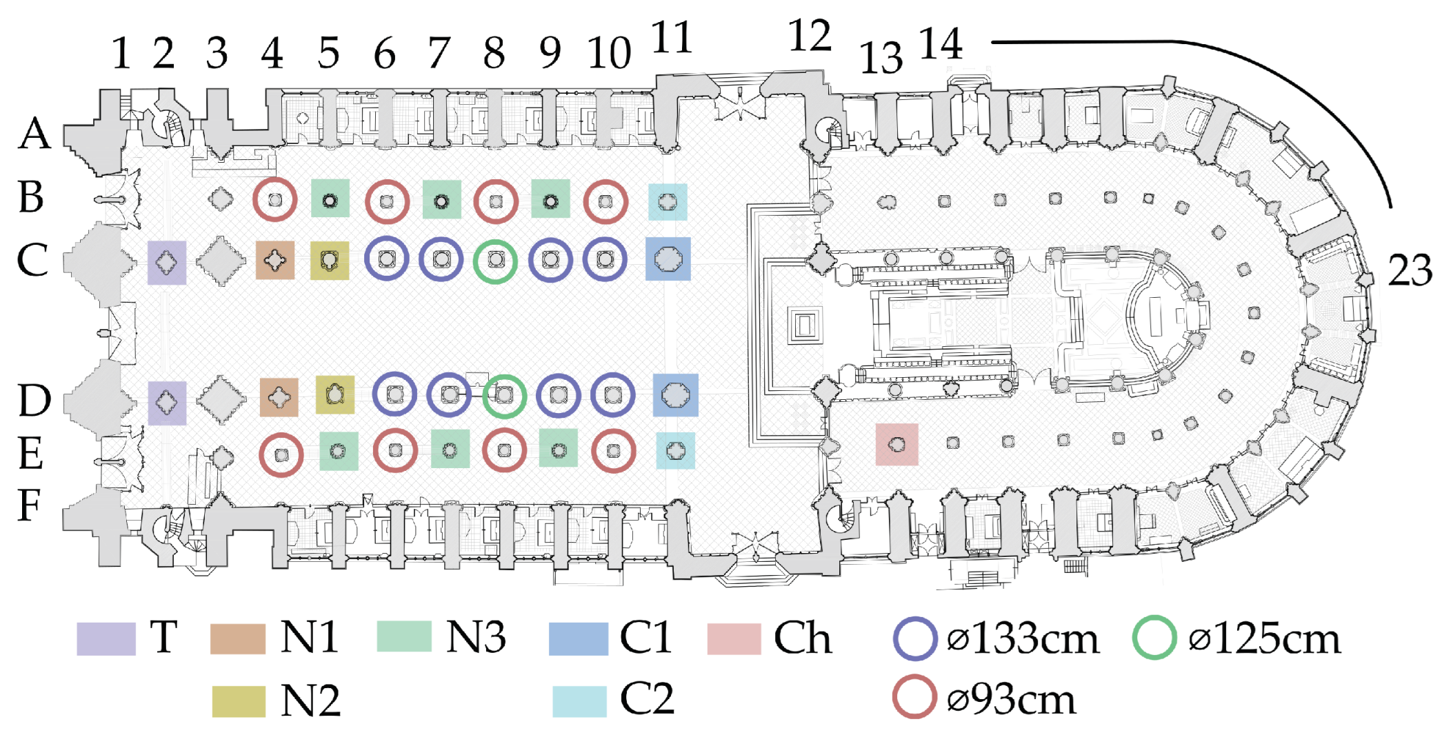
2.1. Columns and Piers of Interest

The many successive construction and renovation campaigns can be seen in part through the geometry of the many piers and columns in the cathedral (Figure 1a). The study of the plinths, bases, and capitals contributed notably to the sequencing of the building site [46]. We restrict ourselves here to the study of the scattering properties of the shafts, being the major part of a column. In total, seven geometries were retained according to architectural criteria, such as their location or frequency, and historical criteria such as their place among the different Gothic styles or their links of influence with later or earlier architectural styles. The groups of columns they define are shown in Figure 2 with a label attributed to each. There are five compound piers, consisting of a core flanked by engaged columns and/or pilasters. These elements extend the arches and ribs to take some of their loads and articulate the structure vertically. These principles were already used in Romanesque architecture [54,55]. Their section is formed of a single closed shape. This distinguishes them from the piers with colonnettes, where long thin en-délit circular columns flank without contact with a central part, in this case, they have a decorative function; two were selected. They are all located in the nave, except one. The columns with circular sections present in this part of the cathedral are also indicated in Figure 2, with their diameters. The piers that are not included in the current study, i.e., not colored, are generally formed with shafts of similar geometries, some of which are visible in [48].

Figure 3 shows the cross-sections of the studied shafts, with their dimensions given in cm. They were drawn based on orthoimages extracted from the interactive 3D visualization environment developed by the Modèles et simulations pour l’architecture et le patrimoine (MAP) laboratory in the framework of the “digital data” working group of the scientific project for the restoration of the cathedral supported by the Centre National de Recherche Scientifique (CNRS) and the French Ministry of Culture [56]. This numerical tool integrates the 3D point clouds obtained by several laser survey campaigns conducted notably by Andrew Tallon in 2010 [47], and also by the company Art Graphique et Patrimoine (AGP) just after the fire of 15 April 2019. They are described in more details in the following.

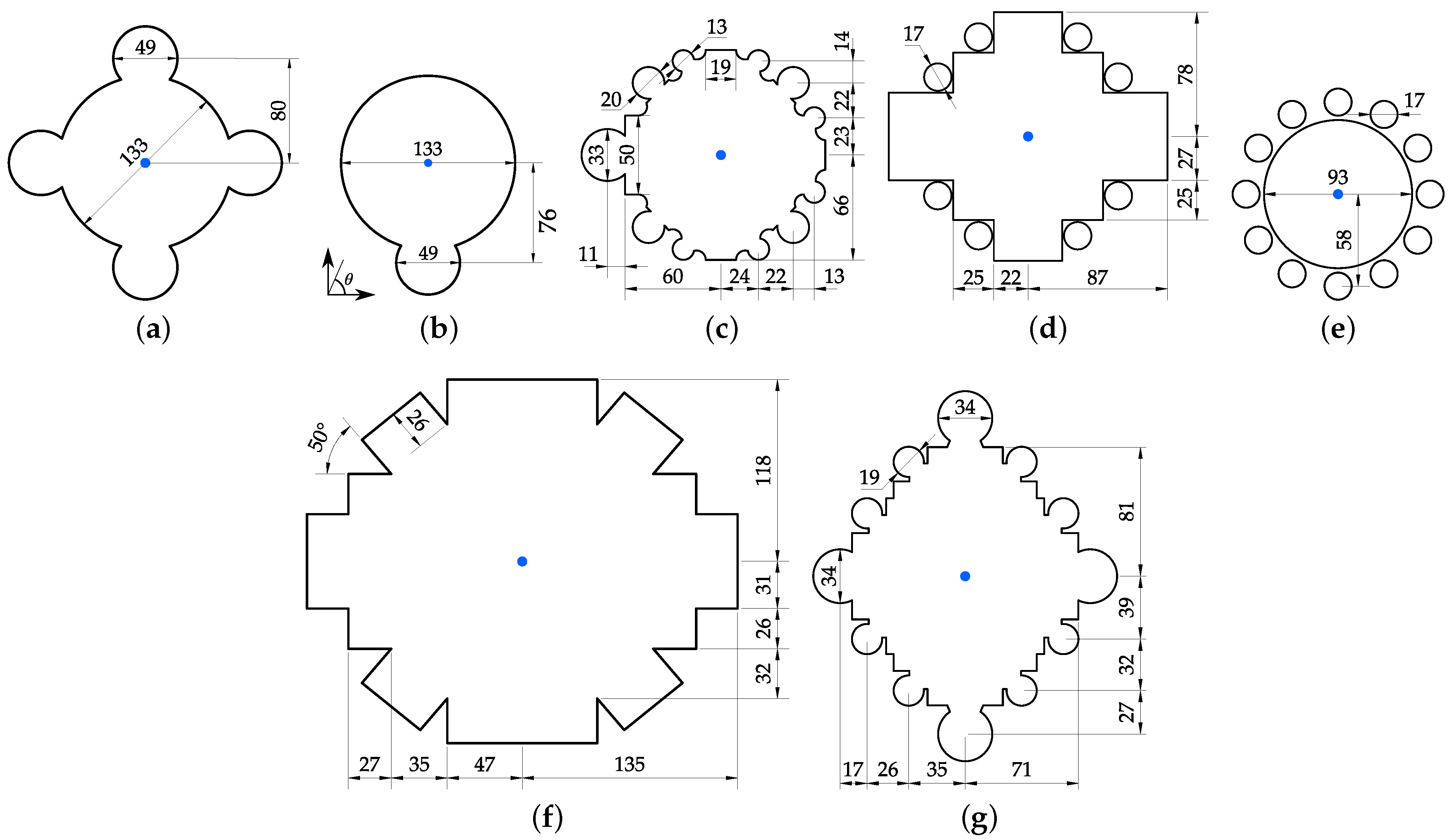
2.1.1. Compound Piers

The first bay of the nave, connecting it with the frontispiece, was built last (see Figure 1a). It resulted in specificity on its columns, because more stiffness was needed in this part, according to Bruzelius [46]. The shafts N1, located at C/D4 in Figure 2, are engaged with four circular colonnettes on a circular core, as shown in Figure 3a. Just besides, the piers N2, located at C/D5, are engaged, with a single one facing the nave (Figure 3b). The central part is the same diameter as the other columns of the nave arcades, except the columns at C/D8 that follow the principle of strong and weak piers, as their diameter is 125 cm. The colonnettes are engaged by less than a quarter of their diameter, penetrating 11 cm and 15 cm, respectively. This type of circular lobe shaft is also found engaged in every responds (Respond: Half-pier or half-column embedded in a wall.). They are piliers cantonnés, a type of pier already used in Romanesque architecture where massive rectangular piers are flanked by semicircular columns, as with Saint-Étienne de Caen Church, Santiago de Compostela or Mainz Cathedrals. Geometries similar to these two couples may be found in other High Gothic cathedrals, as with the naves of Notre-Dame de Chartres and Notre-Dame de Reims, or in the choir of Notre-Dame de Noyon. They are more robust variations of the columns known as “soissonnaises”, which first appeared in Soissons Cathedral, where a single colonnette is engaged in a circular core on the part facing the nave and rises to the vault [57].

Another selected geometry are the transept crossing piers on the nave side C1, located at C/D11. They are actually the union of several pilasters, each one receiving a transverse or diagonal rib of the nave or crossing vaults. At the arcade level, this results in an asterisk-shaped section, as shown in Figure 3f. They are the largest piers of the selection, and, with the two previous ones, they directly surround the nave where listeners are located.

Typical of Gothic architecture, it is also found in the cathedral compound piers formed by a cluster of coursed shafts shaped with relatively thin engaged circular parts that extend vertically the arcs and the ribs of the vaults. The supports of the towers, located at C/D3, are built with this method. Their sides facing the central vessel extend up to high capitals at the base of the sexpartite vaults, forming a diffusing surface close to the Grand Organ. This is also the case for its intermediate piers. The piers T, located at C/D2, are selected to study the influence of such shafts. Their cross-section is shown in Figure 3g. At each corner of the diamond shape is engaged a wider column of diameter 34 cm, and on the sides, there are alternately right corners and engaged colonnettes of diameter 19 cm. This pattern is repeated on the wall and outer aisle responds, between each chapels, of the choir [58].

The eastern transept crossing piers, located at C12 and D12, on either side of the current altar, are the oldest of the building with such shafts. When the chapels of the choir were nearly completed, Pierre de Chelles renewed the eastern wall of the transept around 1315 [59], introducing foliate gables to the arcades of the ambulatory entrance and the piers located at B12 and E12 were modified. The North and South parts are different; the second, probably built in first, is less massive and less prismatic. Their shapes are similar to those of the intermediate piers of the chapels, located from A18 to A23, as well as the responds located in the outer direction to them, at the back of the chapels, and their counterpart in the southern half. The shafts have, as in Early Gothic, engaged columns and colonnettes, but we find some of several diameters revealing a more advanced Gothic style, closer to the flamboyant Gothic, and the corners are no longer all straight, as he introduced curved faces where the colonnettes are flanked. The piers, located at B13 and E13 in the ambulatory, and the second one of the south side arcade, located at D14, were also built around this moment, and are similar. They replaced circular piers following structural problems that led to ruptures, and it is not clear who between Pierre de Chelles and Jean Ravy was leading these repairs [59]. The pier in the southern part of the ambulatory is selected to study a shaft more representative of a latter Gothic style. It is labeled Ch and its cross-section is shown in Figure 3c.

2.1.2. Piers with Detached colonnettes en délit

The use of colonnettes en délit is widespread in the cathedral. They divide the tribune openings, in two in the choir and in three in the nave, except in the first bay. They are in the responds of the nave, in the central vessel from the clerestory (Clerestory: Upper row of bays of a nave located above the triforium and the tribunes.) to the tribunes, extending in a uniform way the ribs of the sexpartite vaults and in the outer aisles. They are 17 cm in diameter. This principle is found at the arcade level on the columns C2, located at B/E11, at the entrance of the double aisles at the western wall of the transept. It is represented in Figure 3d. The prismatic piers formed by the union of the arcades and vaults dosserets (Dosseret: Pilaster used as a straight jamb for an arch.) are supplemented by detached colonnettes at each re-entrant corner, separated by a distance of 1 cm.

Separating the double aisles, every other circular pier N3, located at B/E5/7/9, is surrounded by 12 detached colonnettes, as shown in Figure 3e. Viollet-le-Duc [60] explained this difference with the single circular cylinder neighbors by considerations of structural strength and stability. In particular, since these piers are in line with the most heavily loaded columns of the nave, they had to take the load of the buttresses, which had existed before 1220, and were allowed to counter the thrust from the sexpartite vaults. However, this has been challenged since [58], and Viollet-le-Duc himself acknowledged that they have a decorative function when installed at the responds after settlement of the building. A couple of them are also included among the coursed shafts that form the piers supporting the towers, located at B/E3. Many examples of such elements can be found in other cathedrals at the time, including, not exhaustively, the cathedrals Notre-Dame de Noyon, Saint-Étienne de Bourges, Notre-Dame de Dijon, and Notre-Dame de Laon [61]. Their use facilitated the way in which the walls are vertically articulated, with the vaults compared to coursed shafts with circular shapes, as in the choir responds. They could be manufactured in mass by standard processes while the walls were built with stones cut in regular rectangular shapes [62]. The piers surrounded by colonnettes are also at the origin of a whole architectural style in England [63]. We can give the examples of the Canterbury Cathedral, the Lincoln Cathedral, or the Salisbury Cathedral, where the colonnettes are in marble of a different color from the central part [64].

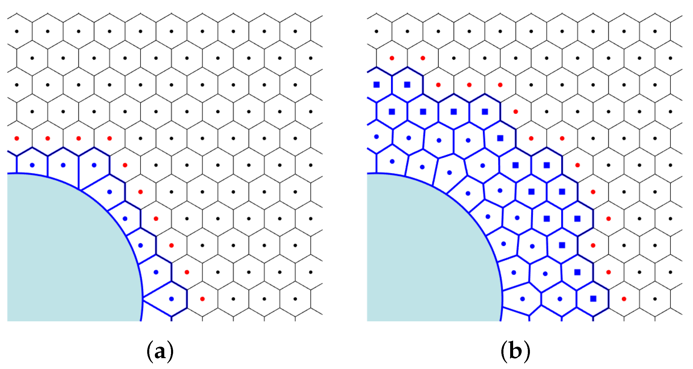
2.2. Numerical Methods

Scattering problems can be treated with numerical simulations such as finite-difference methods, which are particularly convenient for solving the wave equation and thus working directly in the time domain. However, in the context of complex geometries, as studied here, particular care must be taken with the boundary conditions to avoid the staircase approximation usually employed when the numerical scheme is derived from a regular spatial grid. In this study, this issue is addressed by implementing a hybrid time-domain method using finite-difference and finite-volume methods detailed in the following.

The studied objects are relatively long straight cylinders; it is then relevant to restrict the problems to a two-dimensional space. Thus, the second-order wave equation in two space dimensions is solved using a finite difference scheme operating on a hexagonal grid. The Laplacian is approximated by the centered difference operator using seven spatial points: the central point and its six nearest neighbors [65]. Similarly, the time derivative is approximated by a centered finite difference resulting in a fully explicit second-order accurate scheme. The update equation for $p_{i,j}^n$, $\left(i,j\right)\in {\mathbb{Z}}^2$, $n\in \mathbb{N}$, approximating the pressure $p\left(ih{\mathbf{e}}_{\mathbf{1}},jh{\mathbf{e}}_{\mathbf{2}},n\Delta t\right)$ with $\Delta t$ the time step, h the grid spacing, ${\mathbf{e}}_{\mathbf{1}}={\left[\begin{array}{cc}1& 0\end{array}\right]}^T$, ${\mathbf{e}}_{\mathbf{2}}={\left[\begin{array}{cc}-1/2& \sqrt{3}/2\end{array}\right]}^T$, is

$$p_{i,j}^{n+1}=2p_{i,j}^n-p_{i,j}^{n-1}+{\lambda }^2\left[\frac{2}{3}\left(p_{i+1,j}^n+p_{i-1,j}^n+p_{i,j+1}^n+p_{i,j-1}^n+p_{i+1,j+1}^n+p_{i-1,j-1}^n\right)-4p_{i,j}^n\right],$$

(1)

where $\lambda =c\Delta t/h$ is the Courant number. This is a simple way to reduce the numerical dispersion [23] and to improve the isotropy of the propagation, compared to other compact schemes operating on a rectilinear grid [29].

When a wave is scattered by an obstacle, part of it circumvents the latter and propagates as a circumferential wave, so it is crucial to take into account the specific contour geometry of the objects. Depending on the scheme used, a boundary mesh based on a regular grid does not always allow for consistency [66]. This is because using a staircase approximation for a closed curved boundary converges in area but not in perimeter at the limit of small spatial steps [28]. Several locally conformal FD schemes have been proposed [27,67] to handle curved boundaries. Here, the structured hexagonal grid is modified over a thin layer around the object boundaries into an unstructured mesh conforming to it. The approximation of the wave equation on this part of the space is then treated by a finite volume method [68]. The boundary condition of the objects studied are considered to be rigid, which is consistent with the strong impedance contrast existing between air and rocky materials that constitute historic buildings, and the 40 µm average roughness of Lutetian limestone measured in [69]. The update equations in matrix form for the pressures $\mathbf{p}={\left[\begin{array}{ccccc}{p}_1& \cdots & p_l& \cdots & p_N\end{array}\right]}^T$, $l=1,\cdots ,N$, associated with the N finite volume cells are thus

$${\mathbf{p}}^{n+1}=2{\mathbf{p}}^n-{\mathbf{p}}^{n-1}-c^2\Delta t^2{\mathbf{D}}^T\mathbf{D}{\mathbf{p}}^n,$$

(2)

where

$$\mathbf{D}={\mathbf{S}}^{1/2}{\mathbf{H}}^{-1/2}{\mathbf{Q}}^T{\mathbf{V}}^{-1/2},$$

(3)

with $\mathbf{Q}$ is the matrix form of an oriented adjacency tensor $Q_{l,e}$, where $e=1,\dots ,N_e$, $N_e$ is the number of internal edges forming the cells. For a given edge e adjacent to two cells of index $l_e^{+}$ and $l_e^{-}$, such that $l_e^{+}>l_e^{-}$, the tensor is defined as

$$Q_{le}=\left\{\begin{array}{cc}1\hfill & \mathrm{if}l=l_e^{+},\hfill \\ -1\hfill & \mathrm{if}l=l_e^{-},\hfill \\ 0\hfill & \mathrm{otherwise}.\hfill \end{array}\right.$$

(4)

$\mathbf{V}$ is a diagonal matrix with the cell volumes $V_l$, $\mathbf{S}$ and $\mathbf{H}$ are diagonal matrices with the edge lengths $S_e$ and inter-cell distances $H_e$, respectively. $\mathbf{D}$ is the FV approximation of the gradient operation, and ${\mathbf{D}}^T\mathbf{D}$ approximates the Laplacian operation.

The FV mesh is obtained from the Voronoi diagram of the set of grid points enclosing the object completely. The achieved polygons are, in a second step, clipped by the boundaries of the scatterer. An example is shown in Figure 4a. The FV approximation is equivalent to the FD one when applied to a regular mesh [70], as represented with black lines and dots. The red dots are on the FD hexagonal grid. They are used to bound the Voronoi diagram in the outer direction to the scattering object and thus obtain their adjacency relation with the Voronoi cells. It is then possible to establish the discrete Laplacian to link the two meshes when updating the equations.

Depending on its geometry, i.e., whether it is smooth with respect to the spatial step or sharp with re-entrant corners; such a mesh can result in very strict stability conditions in the second case [71], which is not computationally efficient. Therefore, in a third step, a new mesh is generated from the Voronoi diagram of the centroids of the Voronoi polygons obtained previously and clipped as before. This process is repeated to approximate a centroidal Voronoi diagram with Lldoyd’s method [72]. Figure 4b shows the finite volume mesh obtained after 10 iterations. Here, Lldoyd’s method is only applied on the points less than two spatial steps away from the boundary at the first iteration and not on the sites marked with a blue square. In other words, these points remain at their original position on the regular grid, ensuring complete regularity beyond.

Setup

All simulations are performed with a grid spacing about $h=5$ mm in the regular part, corresponding to 10 points per wavelength at 7 kHz. The hybrid mesh is obtained with 5 iterations of Lloyd’s method. Each contour is discretized by a set of linear elements using GMSH (version 4.7.1) [73], so that the error on the perimeter is less than 0.1%. The time step $\Delta t$ is limited by the stability condition from the FV formulation derived in [68], which does not reduce to the proper stability condition for the hexagonal scheme. It is therefore set at

$$\Delta t=min\left\{\frac{2}{\sqrt{{\beta }_{\max }}c},\sqrt{\frac{2}{3}}\frac{h}{c}\right\},$$

(5)

where ${\beta }_{\max }$ is the largest eigenvalue of ${\mathbf{D}}^T\mathbf{D}$. The speed of sound c for the simulations carried out to be compared with the measurements is estimated using [74], according to the temperature and humidity measured in the experimental room. The resulting Courant number $\lambda$ of each simulation is given in

Table 1. Experimental set-ups and parameters for the measurements on scale models with the Courant number $\lambda$ used in each corresponding simulation.

Label (Fig.)	Scale Factor	Incidence Angle ${\mathit{\theta }}_0$	Distance from Center 1		c [m s−1]	$\mathit{\lambda }$
			Source [cm]	Receiver [cm]
N1 (Figure 3b)	1:12	90°	31	307	346.2	0.755
N2 (Figure 3a)	1:12	90°	32	307	345.7	0.751
		45°	32	307	345.8	0.731
C1 (Figure 3f)	1:12	0°	32	306	345.7	0.753
		90°	32	306	346.2	0.742
T (Figure 3g)	1:10	90°	31	319	346.1	0.744
Ch (Figure 3c)	1:10	0°	31	319	346.5	0.743
C2 (Figure 3d)	1:8.5	90°	33	307	346.1	0.753
		0°	33	307	345.9	0.739
N3 (Figure 3e)	1:8.5	0°	33	338	346.6	0.745
		15°	37	317	346.6	0.762

¹ Represented by a blue dot in Figure 3a–e.

. All simulations realized for the time-frequency analysis are performed with $c=344$ m s⁻¹.

The source signal is a Ricker wavelet with a central frequency of 2 kHz injected as a soft source [75] over a line of grid points to have a plane wave incidence. A uniaxial perfectly matched layer is introduced at the end of the computational domain in the direction of propagation of the plane wave. Moreover, periodic boundary conditions are used to prevent edge effects. The scattered field $p_s$ is defined as

$$p_s=p-p_i,$$

(6)

where p is the total field and $p_i$ is the incident field. Therefore, a free-field simulation, without the cylinder, is performed in parallel to the total field simulation, on the regular grid used to generate the hybrid mesh with, consequently, strictly identical parameters, allowing to isolate the scattered field similarly to [24]. Examples of pressure field simulations are included as videos in the Supplementary Materials.

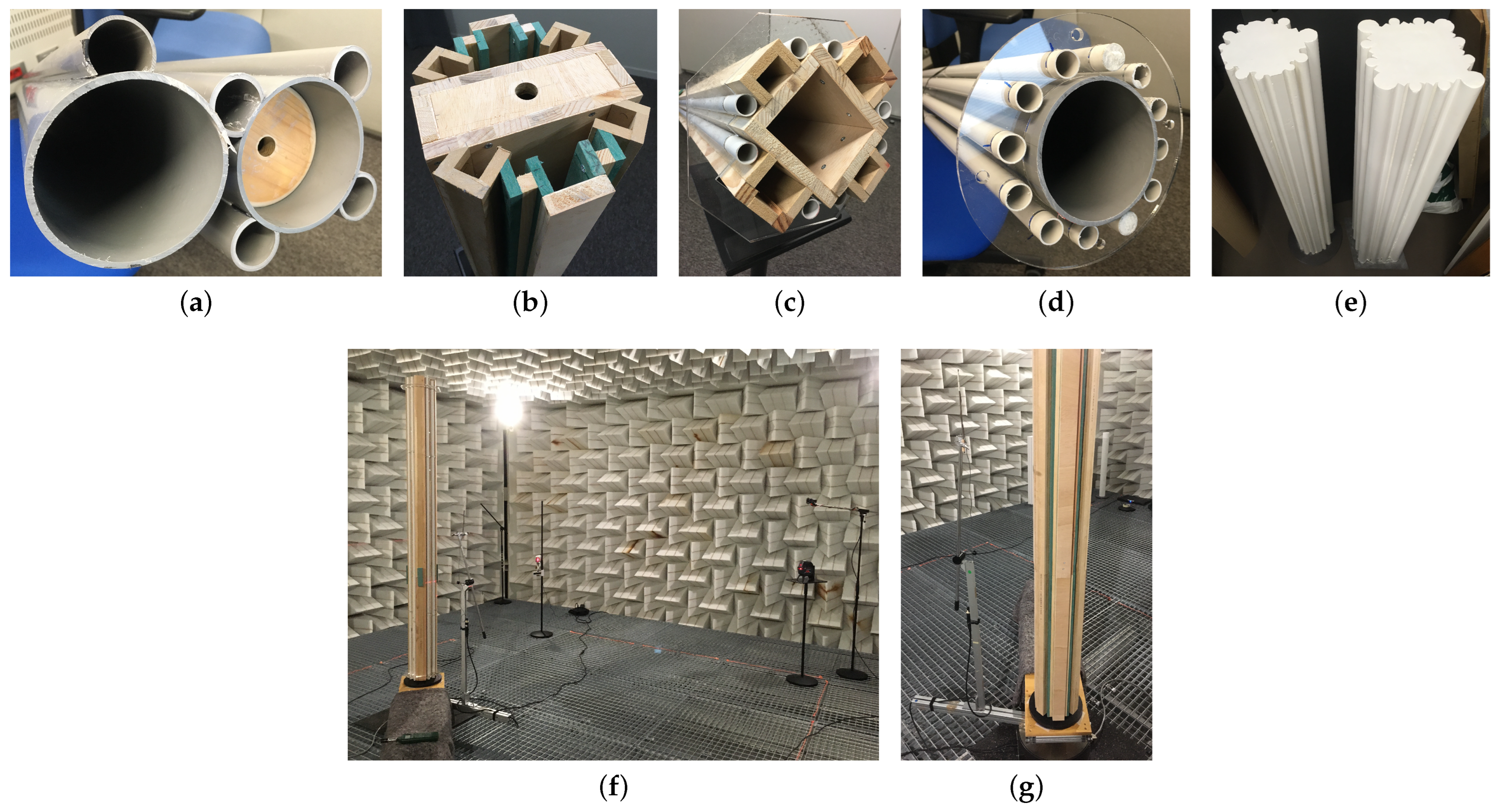
2.3. Experimental Methods

In spite of the progress of numerical methods, physical scale models are still a widespread tool in architectural acoustics, and in particular for investigating the acoustics of complex rooms such as concert halls or for the characterization of scattering from surfaces. They offer the advantage of accounting for all wave phenomena occurring in full-scale problems, provided that they are representative of them. In the case of airborne sound scattering by a rigid object, if the thermo-viscous and molecular relaxation effects are neglected, the full-scale results are obtained, depending on the domain considered, by frequency transposition or time dilation of the scale model results. Moreover, they can be used as validation tools by providing reference results from measurements.

The scattering of the different geometries was measured experimentally by a subtraction method with scale models. They are, for the most part, made of an assembly of long rigid PVC tubes and/or dense wooden boards and cleats, as shown in Figure 5a–d. The detached colonnettes are positioned at the right distance from their core with the help of wedges. Their total length is about 2 m. Both models of compound piers with clustered engaged shafts are made of staff, a plaster-based material. The fresh material is spread in successive layers with a comb whose shape is the negative of one symmetric part of the section. These parts are eventually attached together to form the cylinder, as shown in Figure 5e. Those are 1 m long. Their scaling factor, given in Table 1, is determined by the manufacturing constraints, i.e., according to the standard dimensions of the PVC tubes and wooden cleats, and for those in plaster, it is chosen as a compromise between the size and weight of the model and the minimum size required by the technique to achieve the details.

The measurements were carried out in the anechoic chamber of Sorbonne Université (Figure 5f). The sound field was measured on a circular arc around the cylinder. For that, a microphone was attached to an articulated arm allowing for positioning in space, which was mounted on a turntable (Brüel & Kjær Turntable System Type 9640). The cylinders were positioned on a platform above the turntable that was not in contact with it, to allow the arm with the microphone to rotate around. In practice, the legs of the support platform prevented measurement for about a quarter of a circle (Figure 5g). Since all diffusers have at least one plane of symmetry, recording the signals on an arc greater than a semicircle that includes the forward and backscattering positions allows for full measurement of the scattering in the case where the source is included in this plane of symmetry and orientated towards the center of the scatterer.

The source was a 20 mm diameter dome tweeter (Audax TM020G3) driven by an amplifier (Samson Servo 120a) positioned at a corner of the chamber, as may be seen on the right of Figure 5f. The signals were recorded using a miniature microphone (Feichter Audio M1). Its axis was parallel to the cylinder axis to minimize variations due to its directivity. All were connected to an audio interface (RME Babyface) configured at a sample rate of 192 kHz. The exponential swept sine method [76] was used with signal spanning frequencies from 2 kHz to 95 kHz over 3 s. The exploitable frequency band was eventually identified from 2 kHz to 30 kHz, limited by the source, with a drop in the signal-to-noise ratio (SNR) at 20 kHz. The measurements were carried out with an angular step of 5°, and the emission and acquisition of signals, as well as the control of the turntable, were performed with MATLAB 2020a through an automatic procedure. The source, the microphone, and the cylinder were positioned with the help of laser levels visible in Figure 5f. The different set-ups are summarized in Table 1. The shortest distance from the source to the columns is nearly 3 m, well beyond the Rayleigh distance of the source, $\pi a_{\mathrm{source}}^{2}f/c$, where $a_{\mathrm{source}}$ is the source radius at any frequency f.

For each tested configuration involving a geometry and an angle of incidence, a series of measurements with, then without the cylinder have been made, taking care not to change the positions of the source and the receiver during the removal. It is then possible to isolate the scattered pressure by subtracting the incident pressure to the total pressure recorded respectively without and with the cylinder present. This method is very sensitive to variations of environmental conditions. Changes in temperature and humidity in the chamber, microphone positioning, or response of the equipment due to electrical deviations and Joule heating cause disparities in time and amplitude between measurements. Several methods have been proposed to compensate for them in post-processing [77]. At low-frequency, amplitude variation is the dominant error factor, while at high-frequency, it is the time shift. Here, we compensate only for the difference of time of arrival. It is obtained by a cross-correlation between the free-field signal and the total pressure signal. As it is generally a fraction of a sample, the estimation is refined by interpolation on a Gaussian curve, as proposed in [78]. Since this method is not applicable to signals measured in the shadow zone, these are corrected with the average of the estimated time shifts for the neighboring visible positions of the same series.

3. Results

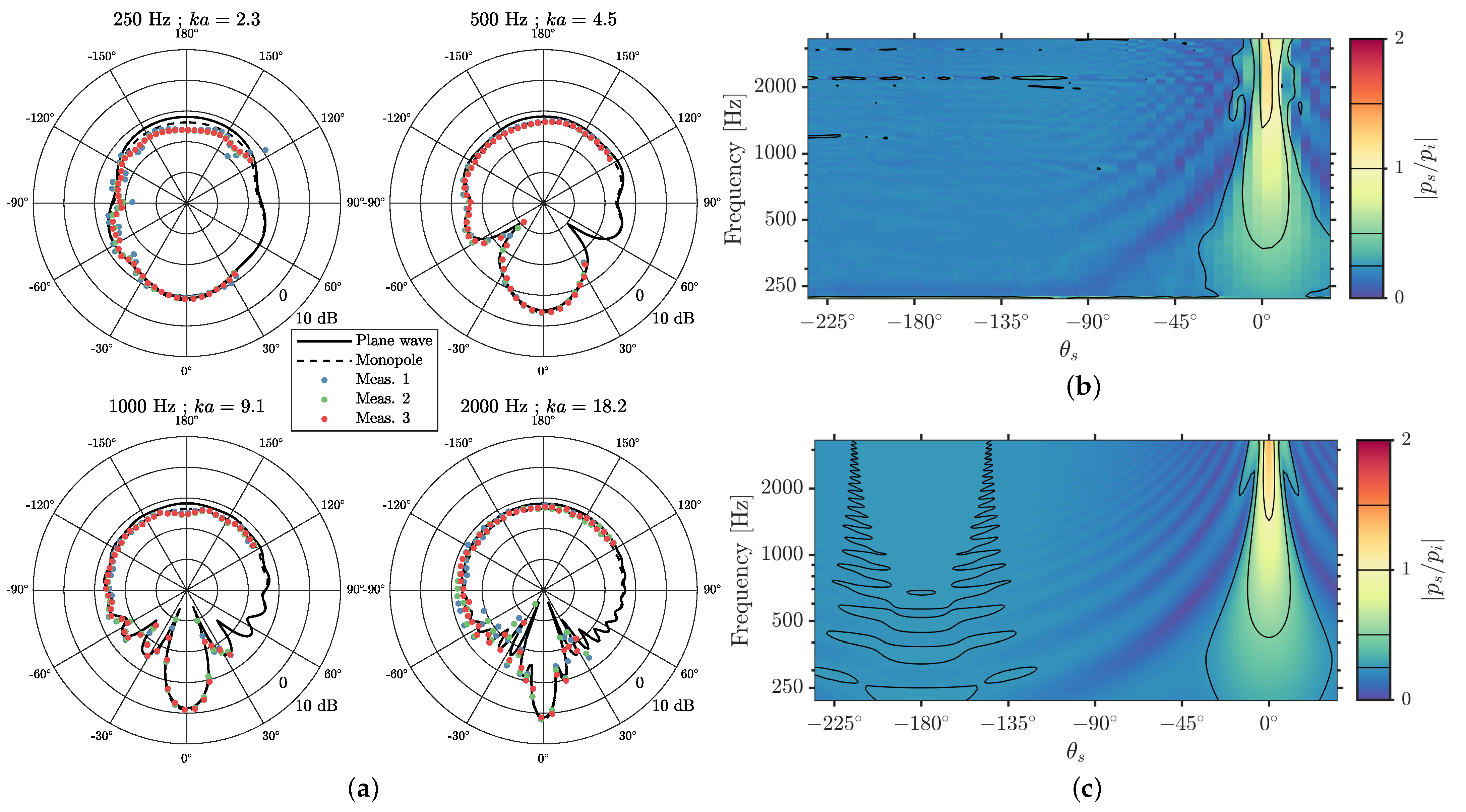
3.1. Validation of the Experimental Methods with a Rigid Circular Cylinder

In order to validate the proposed measuring system and post-processing to obtain the scattered pressure, measurement series have been made with a PVC tube of outer diameter 110 mm to model an infinite rigid circular cylinder. The thickness of the pipe is 3.2 mm, which is sufficient to assume such a boundary condition in the case of airborne propagation [79]. The scale factor is set to 1:9.1 in order that it represents a cylinder of 1 m in diameter at full scale. Three repetitions of the same measurement have been made. The source and microphone positions are not changed between them. They are at 310 cm and 42 cm from the cylinder axis, respectively. The humidity and room temperature have been measured for each repetition. The average estimated speed of sound for the three measurements was 345.5 ± 0.1 m s⁻¹ as the maximum absolute difference. The variations of c between the repeated series are small, so they are compared to the analytic solutions for the plane and spherical incidences calculated with this average value.

Figure 6 compares the measured and analytic results for the scattered sound in the frequency domain. Figure 6a shows the polar diagrams as functions of the scattering angle ${\theta }_s=\theta -{\theta }_0$ of scattered pressure levels relative to the incident field at the discrete scaled frequencies 250 Hz, 500 Hz, 1000 Hz, and 2000 Hz, compared to analytic solutions with plane wave and spherical incidence. The corresponding Helmholtz number $ka$ is also indicated for generalization, where k is the wavenumber and a the cylinder radius. For the source distance chosen, the scattered relative level for the plane wave incidence is about 1.8 dB higher than the spherical incidence in the backscattering direction for all the frequencies considered here. For other angular positions, the differences are lower. In the forward scattering direction, the plane wave incidence leads to a relative scattered level about 0.6 dB lower than the monopole source. Overall, the measurements are in a better agreement with spherical incidence than the plane wave. A very good agreement is observed at 500 Hz and 1000 Hz. At 250 Hz, the back and transverse relative scattered pressure levels are lower than the analytic solutions and the variations between series are high. This is also the case at 2000 Hz in the transverse direction. These frequencies are close to the limit of the sound source where the signal-to-noise ratio is lower, degrading the accuracy. Additionally, the proposed correction for positions in the shadow zone leads to a good estimate, given the excellent agreement found for the forward scattering peak and the observed repeatability between the series. Finally, the rigidity hypothesis for this scale model seems acceptable.

Figure 6b shows the magnitude of the measured scattered pressure relative to the incident pressure for Meas. 3 over all the available frequency ranges, scaled according to the factor, for each angular position. Comparing it to the plane wave solution represented in Figure 6c confirms the underestimation in the backscattering region, and the slight overestimation in the forward direction. The interference pattern in the transverse direction is less visible at high frequency in Figure 6b compared due to the low angular sampling. The drop of signal-to-noise ratio around 20 kHz is visible at the scaled frequency of 2200 Hz, manifested by an horizontal line of high values, mainly over the backscattering positions of the arc. The proposed methods for correcting time shifts appear to be suitable for the visible and shaded positions. In the following, the measurements on the columns of interest are compared to simulation results where the source is a plane wave. The present results show that this assumption is likely to affect mainly the backscattering region.

3.2. Measurements Compared to Simulations

Figure 7 shows the magnitude ratios between the experimentally measured scattered and incident pressures and their numerically simulated counterparts for three of the configurations; results of other configurations are provided in Appendix A. The proposed subtraction method was applied to the signals and the spectra were obtained by Fast Fourier Transform; no correction for excess air absorption is made. The results are compared in the frequency domain and the vertical axis of the surface plots of the experimental results has been scaled according to the factor of each given Table 1. Overall, a good agreement between measurements and simulations can be observed, with constructive and destructive interference appearing within the scattered pressure in steady state match in frequency and space. In particular, the post-processing method for obtaining the scattered pressure in the shadow area based on neighboring positions is suitable, as shown by the comparison of the figures around the direction ${\theta }_s=0$°. In the backscattering region, the magnitude ratios are systematically slightly lower for the measurements on scale models compared to simulations, in agreement with the difference expected between a plane and a spherical incidence. The drop of SNR around 20 kHz is visible in some of the measurement results, manifested by an horizontal line of high values on all positions of the arc; for example, in Figure 7a at around 2400 Hz, or in Figure A2c at around 1700 Hz.

In addition to the error due to the nature of the incident field, other sources are that, for some configurations, the centering of the cylinder and the perpendicularity of the measurement plane to the cylinder axis are not perfectly achieved. For this latter, a part of the wave is thus scattered out of the plane corresponding to oblique incidence. This can be seen when the measured backscattered and forward scattered pressures do not exactly match the expected diametrically opposite directions ${\theta }_s=-180$° and ${\theta }_s=0$°, respectively, that are supposed to be symmetry lines in the figures for such configurations as shown in the simulated results. This is particularly striking in Figure A1e compared to Figure A1f, where the cylinder is probably leaning in the transverse direction. If the cylinder is slightly tilted forward or backward from the source, then it is not visible in this way, but the deflection is still present.

Another one is the geometrical differences that can exist between a hand-made physical scale model and a perfect numerical model. For geometries with outward or inward corners, the scale models will have rounded corners compared to their digital counterparts, where no rounding was introduced afterwards. The effect of rounding corners on the scattered field by concave cylinders with one, two, or four corners has been studied numerically in [80], and they found that maximum differences occurred in the backscattering region with expected dependencies on the radius of curvature, the wavelength, and the angle of incidence, with respect to the position of the corners. Here, the scale models made of staff (Figure 5e) have more rounded edges compared to the wooden models, because of the viscosity of the material having a surface tension, and also affecting both the outer and re-entrant corners. For manufacturing reasons, the angles existing at the intersections of the circles for N2 and N1 (Figure 5a) are also rounded. In addition, for geometries with several elements, a bad straightness, and therefore, the positioning of the small cylinders leads to a different scattering, such as in Figure A2e in comparison to Figure A2f.

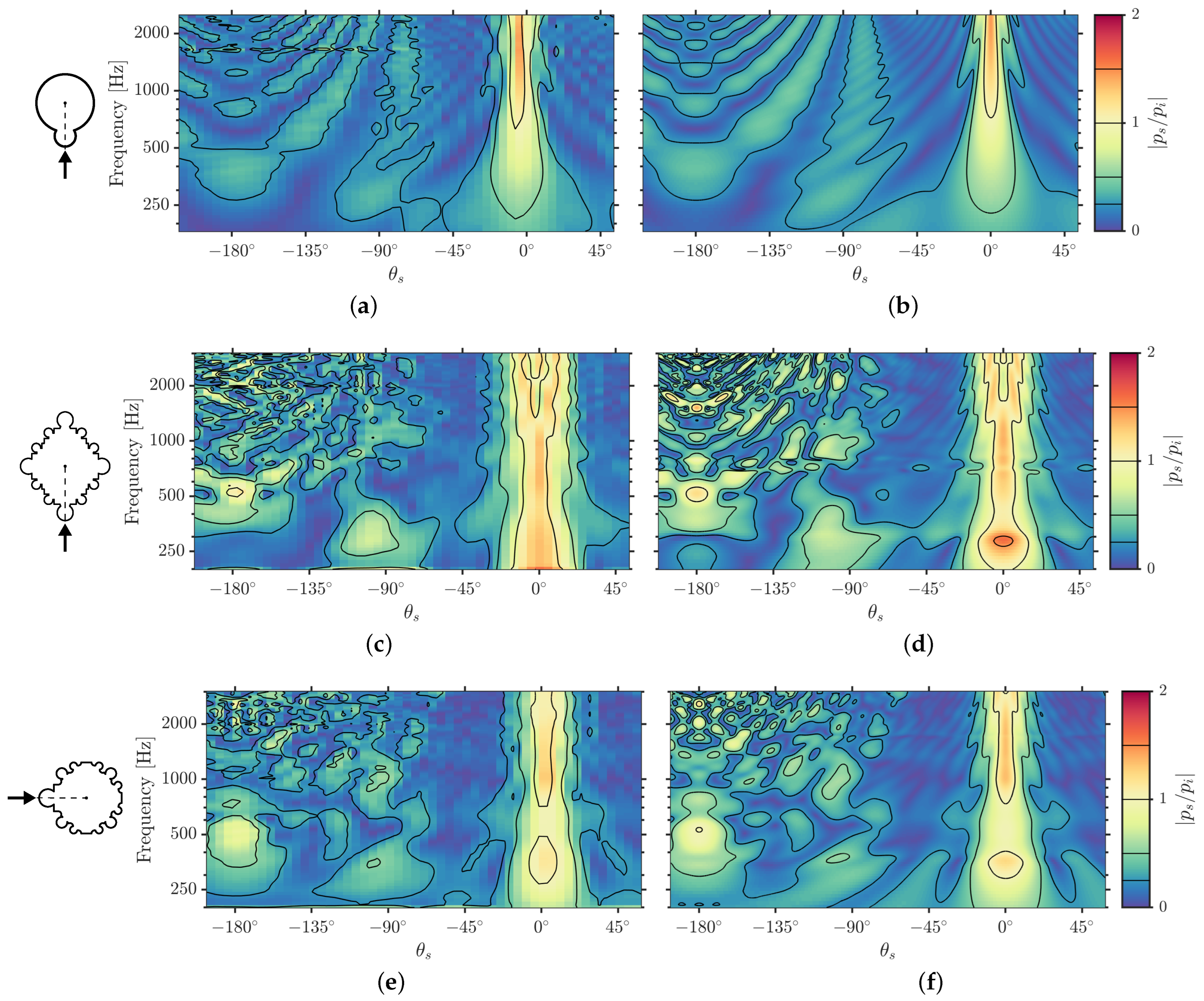
3.3. Simulation Results

Comparisons between measurements and simulations have shown that the latter faithfully represent the situation of a far-field source for the receiver positions considered. They allow to overcome the experimental difficulties and limitations, and thus to enlarge the accessible frequency range. They are nevertheless subject to their own limitations; however, with the parameters used, the scattering can be studied on the octave bands from 125 Hz to 4000 Hz without the numerical dispersion affecting the accuracy significantly. In addition, they are free of background noise and, consequently, allow to reveal the phenomena of low sound levels.

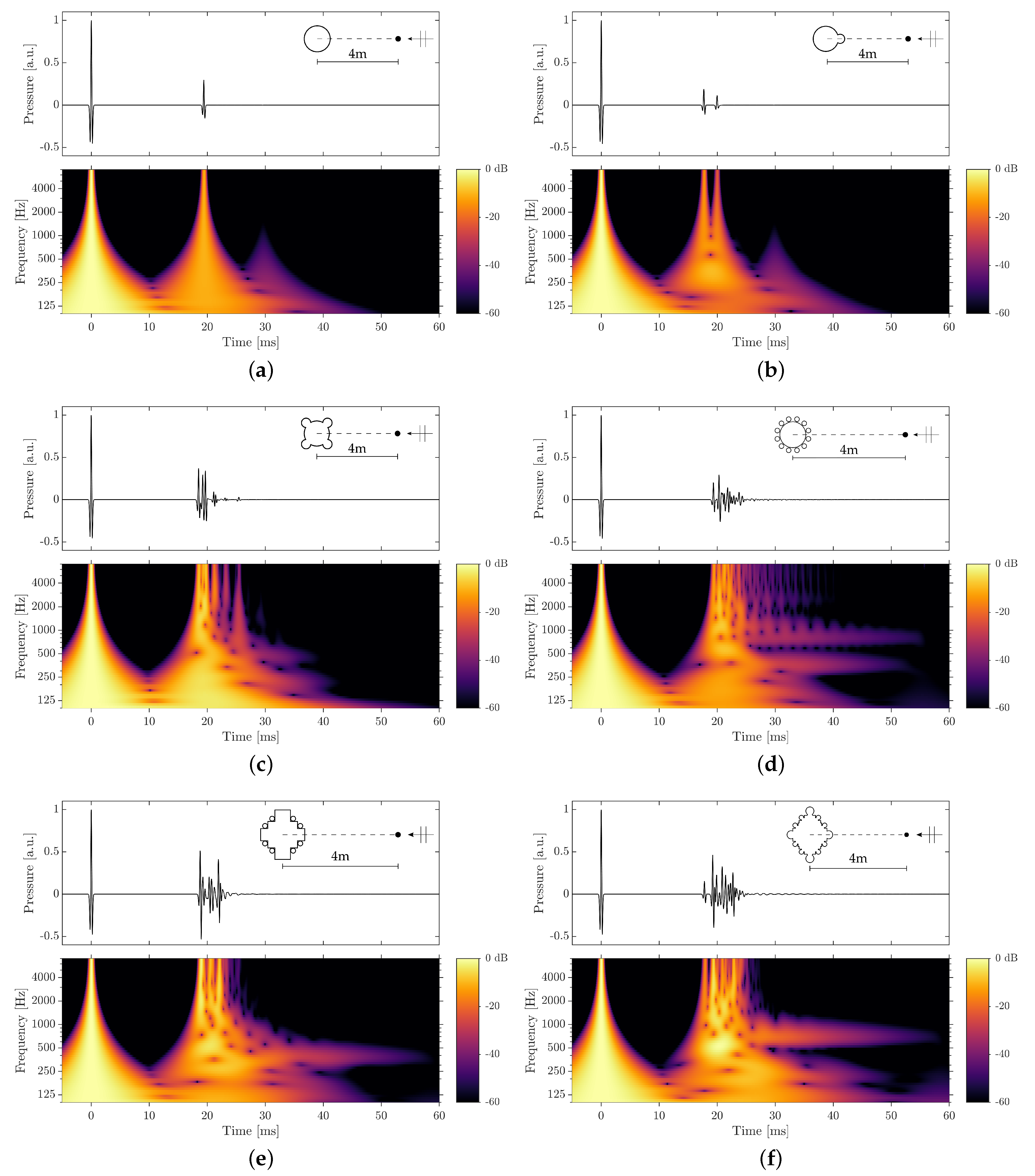
3.3.1. Time-Frequency Analysis

Figure 8 shows the simulated pressure signals at 4 m from the centroid of six different piers in the backscattering direction, and their wavelet scalograms in dB, where each scale has been normalized by the maximum value obtained for the incident pulse. The continuous wavelet transform has been performed using the function cwt implemented in the Wavelet Toolbox version 5.5 of MATLAB 2020a. It has been computed using Morse wavelets, which can be expressed in the frequency domain

$${\mathsf{\Psi }}_{\beta ,\gamma }\left(\omega \right)=H\left(\omega \right)a_{\beta ,\gamma }{\omega }^{\beta }{e}^{-{\omega }^{\gamma }},$$

(7)

where H is the Heaviside step function, $\omega$ is the angular frequency, $a_{\beta ,\gamma }$ is a normalizing constant, $\beta$ is a compactness parameter, and $\gamma$ characterizes the symmetry [81]. The signals are transformed using 10 voices per octave, with parameters set to $\beta \gamma =25$ and $\gamma =3$.

As expected, the temporal structure of the backscattered pulses depends strongly on the geometry of the diffuser. Figure 8a represents the results obtained for a circular cylinder of diameter 133 cm, corresponding to the columns of the nave arcade columns, and to the central part of N1 and N2. In the time domain, the first arrival after the direct sound has a relative peak level of −10.5 dB, which is approximately the value found in the scalogram. A second arrival is visible in the scalogram at low frequency, 30 ms after the direct sound, corresponding to the creeping waves circumventing the cylinder that are strongly attenuated at high frequency. It is not visible in the signal as its relative peak level is −62 dB. For N2 with ${\theta }_0=90$° (Figure 8b), there are two visible arrivals, corresponding to the reflections on the two circular parts constituting the cross-section, with relative peak levels of −14.5 dB and −18.9 dB. The arrival due to the creeping waves is still visible in the scalogram, and has a level and frequency range similar to the circular cylinder. For N1 with ${\theta }_0=45$° (Figure 8c), the pressure signal is composed of a three localized pulses between 18 ms and 20 ms after the direct sound with −9.5 ± 1.1 dB relative peak levels. The latter arrivals are due to higher-order reflections between the different part of the cross-section that account for about 4% of the cumulative energy of the backscattered pulse. Its normalized wavelet scalogram also shows a spreading of low frequency, similarly to the previous geometries. For C2 with ${\theta }_0=90$° (Figure 8e), the wave packet has visible pulses at its onset and offset. They are attributed to the reflections on the plane faces of the cylinder whose normal is colinear with the direction of propagation. In comparison, those of N3 (Figure 8d) and T (Figure 8f) look more like diffuse reflections [82].

Resonance tails are visible in the scalograms of the sections with smaller scale geometrical features, i.e., for N3, C2, and T, thus favoring multiple interactions during scattering. The column N3 (Figure 8d) has two resonances over the considered frequency range. The first one occurs at around the same frequency as C2 (Figure 8e), around 400 Hz. The second one is around 850 Hz and seems to decay slightly slower. The resonance of T (Figure 8f) is around 700 Hz. They all have low amplitudes, so they hardly appear on the linear scale of the pressure signals and account for a very small part of the cumulative energy of the backscattered pulses, less than 0.2% for T, for instance.

3.3.2. Reflected-to-Direct Level Differences

To analyze the reflected signals in a way that is relevant to our perception of sound, the Reflected-to-Direct Level Differences (RDLDs) [38] are calculated for each one-third octave band, in order to better observed the spectral and strength differences depending on the geometry of the cylindrical obstacle, the incidence angle, and the direction of scattering. They are calculated in the frequency domain with the discrete equivalent of

$${\mathrm{RDLD}}_f=20{log}_{10}\sqrt{\frac{1}{f_2-f_1}{\int }_{f_1}^{f_2}{\left|\frac{p_s\left(\omega \right)}{p_i\left(\omega \right)}\right|}^{2}d\omega },$$

(8)

where $f_1$ and $f_2$ are the edge frequencies of the one-third octave band f. Moreover, to be compared with the audibility thresholds reported in the literature, a single-number RDLD [38] is also calculated, taking into account the spectral sensitivity of the ear, with

$$\mathrm{RDLD}=10{log}_{10}\left(\frac{{\sum }_{f=1}^N{10}^{\frac{{\mathrm{RDLD}}_f+T_{W,f}}{10}}}{{\sum }_{f=1}^N{10}^{\frac{T_{W,f}}{10}}}\right),$$

(9)

where ${\mathrm{RDLD}}_f$ are the one-third octave band RDLDs, and $f=1,\dots ,N$, and $T_{W,f}$ are the weights obtained by inverting the equal loudness curve at 40 phons according to ISO 226:2003. Note that no additional weighting is applied, contrary to [38], which is equivalent to considering a flat source magnitude spectrum.

Figure 9 represents the results obtained for N2, C1, C2, and N3 for two incidence angles for each one. We recall that they are derived from simulations representing the experimental set-ups reported in Table 1, where the distances of the receivers to the center of the section are indicated for each one. The one-third octave band RDLDs are shown on a semicircle only, since the configurations are symmetrical. Moreover, the RDLDs for the positions located in shadow zone are also represented; however, they can not be interpreted as such, because of the interference between the incident and scattered pressures occurring in this region.

For the piers N2, the two incidence angles considered result in strong spectral and strength differences across the scattering directions, as shown in Figure 9a. For ${\theta }_0=90$°, the overall RDLDs represented in Figure 9b are around 3 dB higher in the transverse directions compared to ${\theta }_0=45$°. For the piers C1, the RDLDs are very similar, up to 1 kHz, as shown in Figure 9c. Above, the large planar parts of the section favor some directions, according to ray acoustics. These particular directions are therefore highlighted in the overall RDLDs, represented in Figure 9d, where they found their second maximum at around $-4$ dB and $-6$ dB for ${\theta }_0=90$° and 0°, respectively. Their maximum of about 2 dB is found in the backscattering direction, as these incidences are normal to the large plane faces of the cylinders. This is also the case for C2, as shown in Figure 9e, where a positive value of nearly 1 dB is found in the backscattering direction for ${\theta }_0=0$°. For the two incidences considered, the overall RDLDs, represented in Figure 9f, differ mainly in this region, for ${\theta }_s\ge 150$°. Compared to the other section, the RDLDs for N3 seems to depend less on the incidence angle, as shown in Figure 9g.

4. Discussion

4.1. Gothic Piers as Volumetric Diffusers

The function of a surface diffuser is to redirect a sound wave in directions other than the specular one, and to spread it out in time. From these perspectives, a simple circular cylinder alone achieves the spatial spreading, but is not really a good diffuser as it produces a high-pass strongly correlated reflection in the backscattering region [1]. Moreover, its finite size allows it to interact only in a limited way with the wave that impinges on it. Even in its resonant regime, we have seen that the circumferential waves have a very low level and only exist at low frequency. But as soon as discontinuities are included in the geometry, they are potential sources of scattering that produce additional wavefronts.

The compound piers studied here are all concave and some of them are star-shaped. This allows potentially several interactions of a wave scattered by a part of a shape with another of these parts. This is also true for the piers with colonnettes C2 and N3, especially as the small cylinders are close to the central part and to each other. This effect is particularly visible through the existence of resonance frequencies revealed for the latter, as well as for the compound piers with geometric elements of small size, such as T. They are probably the result of coupling between the small cavities formed on the surface of the cylinders creating surface waves, as described in [83,84]. They are, by definition, localized in frequency, and in the cases studied here, count very little for the total energy of the reflections. However, around these frequencies, where the wavelengths are of the order of magnitude of the geometrical elements, i.e., up to about 1 kHz for the geometries considered here, the scattered power is increased without strongly favoring any particular direction. Contrary to beyond, in the limit of small wavelengths, the scattering directions can be determined according to the acoustic ray model, and the overall scattered power is related to the size of the shadow. See [85] for more detailed simulation results of different column geometries analyzed in terms of classical scattering quantities.

We have considered here the obstacles alone, but one may wonder if volumetric diffusion could be possible by multiple scattering between columns. In the cathedral, the piers of the nave are approximately 5.5 m between centers. Therefore, based on the RDLDs obtained, following the decreasing of intensity of a spherical wavefront, the level of a re-scattered wave would be too low compared to the other wall reflections. However, this is valid for a far field source, and it would be interesting to study the effect of an obstacle near a source for a distant listener. Moreover, their influence on the late reverberation, especially on the modes at low frequency, could also be a topic future investigations, considering that, in this case, an image-source of a high order of reflections has interacted with a lot of small obstacles, similar to the propagation within a sonic crystal.

4.2. Audibility of Scattering by Cylindrical Obstacles

The simulations assumed a source positioned at infinity; however, they were shown to be equivalent to the experiments where the source was in the far field, at about 30 m at full scale, and as the receiver is near the obstacle, about 3 m from their center here. This is even more true for the transverse directions, which better correspond to a listening situation with a listener facing the source and with an obstacle near him on its side. In this case, the results presented in Figure 9 indicate that the reflections have sufficient levels to be audible. For the configurations shown here, RDLDs in the direction ${\theta }_s=90$° are greater than −20 dB, which is approximately the thresholds of audibility reported in [38] or the criterion used in [6]. They are between −15 dB and −10 dB, except for C1, where values exist up to −6 dB and −4 dB, for ${\theta }_0=0$° and 90°, and ${\theta }_s=95$° and 113°, respectively.

For such levels, the reflections are audible through changes in coloration rather than loudness. Humans are more sensitive to spectral overlap below 1 kHz [31], which is the range that is best scattered in all directions. Furthermore, in a binaural context, it has been shown that a reflection coming from a lateral direction was more audible than if it came from the same direction or from behind [30,35,36]. However, as already mentioned, for positions more distant in the transverse directions, the decreasing of intensity becomes important enough so that the reflected wave becomes undetectable. Comparing the one-third octave band RDLDs between piers, the spectral differences seem significant enough to discriminate between these reflections. Sound examples of impulses are included in the Supplementary Materials for back and transverse scattering. With preliminary listening, columns inducing diffuse reflections are discernible from a simple circular cylinder, in agreement with the results of [44], but these are monoaural responses and further perceptual studies, and measurements on scale models or three-dimensional simulations of the binaural responses, for example, would be necessary to be able to conclude as to the other shapes between them, in scenarios approaching real conditions for isolated columns.

A listener in the cathedral receives several early reflections, from the columns, but also from the walls. The question arises of a possible masking happening systematically for the positions considered here. For a source located in the choir between the stalls, the reflection off the side wall arrives between approximately 25 ms to 60 ms for the receivers located respectively from the back to the front of the nave. This leaves an interval before which these early column reflections can be significant. Furthermore, if we consider a realistic source, the relative positions will be decisive. Based on scattering theory, a spherical or cylindrical source will be scattered more in the forward and backward directions, and less transversely, compared to a plane wave incidence, and the closer it is, the greater the effect [86]. However, such sources also imply a decay of intensity due to the spatial spread of their wavefront, which could result in a lower relative level of the reflections [6]. Further investigations on room impulse responses and simulations could evaluate these effects. Moreover, several studies have investigated the effect of surface diffusers [10,11,12,13,14] or columns [15] on room acoustic parameters in concert halls, and it would be interesting to conduct similar studies, especially in relation to the previous discussions on the relative positions of the source, obstacles, and listener, and on their collective effects.

5. Conclusions

The purpose of this work was to investigate the sound scattering by obstacles of complex geometries that are the piers and columns of the Cathédrale Notre-Dame de Paris. This heritage monument has evolved across the centuries, and is marked by several Gothic styles, which allowed us to select typical geometries that are relatively different, reflecting the evolution of this medieval architecture. Their scattering has been simulated up to 6 kHz using a low dispersion and anisotropy finite difference scheme with a pulse excitation. It is modified according to the formalism of the finite volumes around the boundaries to conform to it and to avoid the staircase approximation. The method has been validated by comparison with measurements on scale models and analytic models.

A plane wave incidence has been considered in the simulations, and has been shown to be close to the experimental measurements in the case of a far field source and a receiver close to the cylinder. The simulated scattered fields were consequently analyzed in terms of perceptually relevant quantities. Similarly to reflectors, the reflections from columns and piers are limited by their finite size. However, due to their early arrival before most wall reflections, the scattered field at the evaluated positions revealed that these obstacles could produce audible reflections over all scattering directions, based on thresholds reported in the literature. The temporal spreading strongly depends on the scatterer, i.e., the piers’ form. Those with small geometrical features have the ability to produce diffuse reflections similarly to surface diffusers. Low level resonances due to complex forms have also been revealed; however, they represent a very small part of the total reflected energy. Strong spectral differences were observed between piers, such that it is likely possible to be able to discriminate between their reflections. Further studies could evaluate more realistic scenarios with a spherical source and different relative distances between the latter, the obstacle and the listener, numerically and with perceptual testings.

References

1. Cox, T.; D’Antonio, P. Acoustic Absorbers and Diffusers: Theory, Design and Application; CRC Press: Boca Raton, FL, USA, 2016. [Google Scholar] [CrossRef]
2. Rindel, J.H. Design of new ceiling reflectors for improved ensemble in a concert hall. Appl. Acoust. 1991, 34, 7–17. [Google Scholar] [CrossRef]
3. Bradley, D.T.; Müller-Trapet, M.; Adelgren, J.; Vorländer, M. Comparison of Hanging Panels and Boundary Diffusers in a Reverberation Chamber. Build. Acoust. 2014, 21, 145–152. [Google Scholar] [CrossRef]
4. Rindel, J.H. Attenuation of Sound Reflections due to Diffraction. In Proceedings of the Nordic Acoustical Meeting, Aalborg, Denmark, 20–22 August 1986. [Google Scholar]
5. Szeląg, A.; Kamisiński, T.; Lewińska, M.; Rubacha, J.; Pilch, A. The Characteristic of Sound Reflections from Curved Reflective Panels. Arch. Acoust. 2014, 39, 549–558. [Google Scholar] [CrossRef]
6. Rathsam, J.; Wang, L.M. Planar Reflector Panels with Convex Edges. Acta Acust. United Acust. 2010, 96, 905–913. [Google Scholar] [CrossRef]
7. Medwin, H.; Clay, C.S. Fundamentals of Acoustical Oceanography; Applications of Modern Acoustics, Academic Press: San Diego, CA, USA, 1998. [Google Scholar] [CrossRef]
8. Standard ISO 17497-1:2004; Acoustics—Sound-Scattering Properties of Surfaces—Part 1: Measurement of the Random-Incidence Scattering Coefficient in a Reverberation Room. International Organization for Standardization: Geneva, Switzerland, 2004.
9. Standard ISO 17497-2:2012; Acoustics—Sound-Scattering Properties of Surfaces—Part 2: Measurement of the Directional Diffusion Coefficient in a Free Field. International Organization for Standardization: Geneva, Switzerland, 2012.
10. Ryu, J.K.; Jeon, J.Y. Subjective and objective evaluations of a scattered sound field in a scale model opera house. J. Acoust. Soc. Am. 2008, 124, 1538–1549. [Google Scholar] [CrossRef]
11. Jeon, J.Y.; Jo, H.I.; Seo, R.; Kwak, K.H. Objective and subjective assessment of sound diffuseness in musical venues via computer simulations and a scale model. Build. Environ. 2020, 173, 106740. [Google Scholar] [CrossRef]
12. Kim, Y.H.; Kim, J.H.; Jeon, J.Y. Scale Model Investigations of Diffuser Application Strategies for Acoustical Design of Performance Venues. Acta Acust. United Acust. 2011, 97, 791–799. [Google Scholar] [CrossRef]
13. Shtrepi, L.; Astolfi, A.; Pelzer, S.; Vitale, R.; Rychtáriková, M. Objective and perceptual assessment of the scattered sound field in a simulated concert hall. J. Acoust. Soc. Am. 2015, 138, 1485–1497. [Google Scholar] [CrossRef]
14. Shtrepi, L.; Astolfi, A.; Puglisi, G.E.; Masoero, M.C. Effects of the Distance from a Diffusive Surface on the Objective and Perceptual Evaluation of the Sound Field in a Small Simulated Variable-Acoustics Hall. Appl. Sci. 2017, 7, 224. [Google Scholar] [CrossRef]
15. Suzumura, Y.; Sakurai, M.; Ando, Y.; Yamamoto, I.; Iizuka, T.; Oowaki, M. An evaluation of the effects of scattered reflections in a sound field. J. Sound Vib. 2000, 232, 303–308. [Google Scholar] [CrossRef]
16. Strutt, H.J.X. On the light from the sky, its polarization and colour. Lond. Edinb. Dublin Philos. Mag. J. Sci. 1871, 41, 107–120. [Google Scholar] [CrossRef]
17. Morse, P.; Ingard, K. Theoretical Acoustics; International Series in Pure and Applied Physics; Princeton University Press: Princeton, NJ, USA, 1986. [Google Scholar]
18. Bowman, J.; Senior, T.; Uslenghi, P.; Asvestas, J. Electromagnetic and Acoustic Scattering by Simple Shapes; Taylor & Francis: Abingdon, UK, 1988. [Google Scholar]
19. Hughes, R.J.; Angus, J.A.S.; Cox, T.J.; Umnova, O.; Gehring, G.A.; Pogson, M.; Whittaker, D.M. Volumetric diffusers: Pseudorandom cylinder arrays on a periodic lattice. J. Acoust. Soc. Am. 2010, 128, 2847–2856. [Google Scholar] [CrossRef]
20. Yashiro, K.; Ohkawa, S. Boundary element method for electromagnetic scattering from cylinders. IEEE Trans. Antennas Propag. 1985, 33, 383–389. [Google Scholar] [CrossRef]
21. Liu, Y. On the BEM for acoustic wave problems. Eng. Anal. Bound. Elem. 2019, 107, 53–62. [Google Scholar] [CrossRef]
22. Ihlenburg, F. (Ed.) Finite Element Analysis of Acoustic Scattering; Springer: Berlin/Heidelberg, Germany, 1998. [Google Scholar] [CrossRef]
23. Taflove, A.; Hagness, S. Computational Electrodynamics: The Finite-Difference Time-Domain Method; Artech House Antennas and Propagation Library, Artech House: Norwood, MA, USA, 2005. [Google Scholar]
24. Redondo, J.; Picó, R.; Roig, B.; Avis, M.R. Time Domain Simulation of Sound Diffusers Using Finite-Difference Schemes. Acta Acust. United Acust. 2007, 93, 611–622. [Google Scholar]
25. Hoare, S.; Murphy, D. Prediction of scattering effects by sonic crystal noise barriers in 2d and 3d finite difference simulations. In Proceedings of the Acoustics 2012, Nantes, France, 23–27 April 2012; Société Française d’Acoustique, Paris, France, 2012. [Google Scholar]
26. Redondo, J.; Picó, R.; Sánchez-Morcillo, V.J.; Woszczyk, W. Sound diffusers based on sonic crystals. J. Acoust. Soc. Am. 2013, 134, 4412–4417. [Google Scholar] [CrossRef]
27. Tornberg, A.K.; Engquist, B. Consistent boundary conditions for the Yee scheme. J. Comput. Phys. 2008, 227, 6922–6943. [Google Scholar] [CrossRef]
28. Bilbao, S.; Hamilton, B.; Botts, J.; Savioja, L. Finite Volume Time Domain Room Acoustics Simulation under General Impedance Boundary Conditions. IEEE/ACM Trans. Audio Speech Lang. Process. 2016, 24, 161–173. [Google Scholar] [CrossRef] [Green Version]
29. Hamilton, B.; Bilbao, S. Hexagonal vs. rectilinear grids for explicit finite difference schemes for the two-dimensional wave equation. J. Acoust. Soc. Am. 2013, 133, 3532. [Google Scholar] [CrossRef]
30. Olive, S.E.; Toole, F.E. The Detection of Reflections in Typical Rooms. J. Audio Eng. Soc. 1988, 37, 539–553. [Google Scholar]
31. Buchholz, J.M. A quantitative analysis of spectral mechanisms involved in auditory detection of coloration by a single wall reflection. Hear. Res. 2011, 277, 192–203. [Google Scholar] [CrossRef] [PubMed]
32. Burgtorf, W.; Oehlschlägel, H.K. Untersuchungen über die richtungsabhängige Wahrnehmbarkeit verzögerter Schallsignale. Acta Acust. United Acust. 1964, 14, 254–266. [Google Scholar]
33. Seraphim, H. Über die Wahrnehmbarkeit mehrerer Rückwürfe von Sprachschall. Acta Acust. United Acust. 1961, 11, 80–91. [Google Scholar]
34. Brunner, S.; Maempel, H.J.; Weinzierl, S. On the Audibility of Comb Filter Distortions. In Proceedings of the 122nd AES Convention, Vienna, Austria, 5–8 May 2007; Audio Engineering Society: New York, NY, USA, 2007. [Google Scholar]
35. Begault, D.R.; McClain, B.U.; Anderson, M.R. Early Reflection Thresholds for Anechoic and Reverberant Stimuli within a 3-D Sound Display. In Proceedings of the 18th International Congress on Acoustics (ICA04), Kyoto, Japan, 4–9 April 2004. [Google Scholar]
36. Zhong, X.; Guo, W.; Wang, J. Audible Threshold of Early Reflections with Different Orientations and Delays. Sound Vib. 2018, 52, 18–22. [Google Scholar] [CrossRef]
37. Walther, A.; Robinson, P.W.; Santala, O. Effect of spectral overlap on the echo suppression threshold for single reflection conditions. J. Acoust. Soc. Am. 2013, 134, EL158–EL164. [Google Scholar] [CrossRef]
38. Pelegrín-García, D.; Rychtáriková, M. Audibility Thresholds of a Sound Reflection in a Classical Human Echolocation Experiment. Acta Acust. United Acust. 2016, 102, 530–539. [Google Scholar] [CrossRef]
39. Pelegrín-García, D.; Rychtáriková, M.; Glorieux, C. Single Simulated Reflection Audibility Thresholds for Oral Sounds in Untrained Sighted People. Acta Acust. United Acust. 2017, 103, 492–505. [Google Scholar] [CrossRef]
40. Robinson, P.W.; Walther, A.; Faller, C.; Braasch, J. Echo thresholds for reflections from acoustically diffusive architectural surfaces. J. Acoust. Soc. Am. 2013, 134, 2755–2764. [Google Scholar] [CrossRef]
41. Wendt, F.; Höldrich, R. Precedence effect for specular and diffuse reflections. Acta Acust. 2021, 5, 1. [Google Scholar] [CrossRef]
42. Kleiner, M.; Svensson, P.; Dalenbäck, B.I. Auralization of qrd and other diffusing surfaces using scale modelling. In Proceedings of the 93rd AES Convention, San Francisco, CA, USA, 1–4 October 1992; Audio Engineering Society: New York, NY, USA. [Google Scholar]
43. Meyer, J.; Savioja, L.; Lokki, T. A case study on the perceptual differences in finite-difference time-domain-simulated diffuser designs. In Proceedings of the 146th AES Convention, Dublin, Ireland, 20–23 March 2019; Audio Engineering Society: New York, NY, USA. [Google Scholar]
44. Kritly, L.; Sluyts, Y.; Pelegrín-García, D.; Glorieux, C.; Rychtáriková, M. Discrimination of 2D wall textures by passive echolocation for different reflected-to-direct level difference configurations. PLoS ONE 2021, 16, e0251397. [Google Scholar] [CrossRef]
45. Aubert, M.; Vitry, P. La Cathédrale Notre-Dame de Paris: Notice Historique et Archéologique; Notices Historiques et Archéologiques sur les Grands Monuments; D.-A. Longuet: Paris, France, 1919. [Google Scholar]
46. Bruzelius, C. The Construction of Notre-Dame in Paris. Art Bull. 1987, 69, 540–569. [Google Scholar] [CrossRef]
47. Sandron, D.; Tallon, A.; Cook, L. Notre Dame Cathedral: Nine Centuries of History; Penn State University Press: University Park, PA, USA, 2020. [Google Scholar] [CrossRef]
48. Celtibère, M.; Lemercier, M.; Hibon, A.; Ribaud, A.; Normand, A.; Bisson, B. Monographie de Notre-Dame de Paris et de la Nouvelle Sacristie de MM. Lassus et Viollet-Le-Duc; A. Morel: Paris, France, 1853. [Google Scholar]
49. Mullins, S.S.; Canfield-Dafilou, E.K.; Katz, B.F.G. The development of the early acoustics of the chancel in Notre-Dame de Paris: 1160–1230. In Proceedings of the 2nd Symposium: The Acoustics of Ancient Theatres, Verona, Italy, 6–8 July 2022. [Google Scholar]
50. Lassus, J.B.A.; Viollet-le-Duc, E.E. Projet de Restauration de Notre-Dame de Paris par MM. Lassus et Viollet-Leduc: Rapport…Annexé au Projet de Restauration, Remis le 31 Janvier 1843; Imprimerie de Mme de Lacombe: Paris, France, 1843. [Google Scholar]
51. Travaux de Notre-Dame de Paris—Journal des Travaux 1844–1865. Available online: https://mediatheque-patrimoine.culture.gouv.fr/travaux-de-notre-dame-de-paris-1844-1865 (accessed on 1 June 2022).
52. Postma, B.N.; Katz, B.F.G. Acoustics of Notre-Dame Cathedral de Paris. In Proceedings of the 22nd International Congress on Acoustics (ICA), Buenos Aires, Argentina, 5–9 September 2016; pp. 5–9. [Google Scholar]
53. Katz, B.F.G.; Weber, A. An acoustic survey of the Cathédrale Notre-Dame de Paris before and after the fire of 2019. Acoustics 2020, 2, 791–802. [Google Scholar] [CrossRef]
54. Hoey, L.R. Pier Form and Vertical Wall Articulation in English Romanesque Architecture. J. Soc. Archit. Hist. 1989, 48, 258–283. [Google Scholar] [CrossRef]
55. Thurlby, M. Aspects of the architectural history of Kirkwall Cathedral. Proc. Soc. Antiqu. Scotl. 1998, 127, 855–888. [Google Scholar]
56. CNRS/MC. Chantier Scientifique Notre-Dame de Paris. Available online: https://www.notre-dame.science/ (accessed on 1 June 2022).
57. Klein, B. Naissance et formation de l’architecture gothique en France et dans les pays limitrophes. In L’art Gothique, Architecture-Sculpture-Peinture; Toman, R., Ed.; Könemann: Köln, Germany, 1999; Chapter 3; pp. 28–114. [Google Scholar]
58. Murray, S. Notre-Dame of Paris and the Anticipation of Gothic. Art Bull. 1998, 80, 229–253. [Google Scholar] [CrossRef]
59. Davis, M.T. Splendor and Peril: The Cathedral of Paris, 1290–1350. Art Bull. 1998, 80, 34–66. [Google Scholar] [CrossRef]
60. Viollet-le-Duc, E.E. Dictionnaire Raisonné de l’Architecture Française du XIe au XVIe Siècle; B. Bance: Paris, France, 1859. [Google Scholar]
61. Fernie, E. La fonction liturgique des piliers cantonnés dans la nef de la cathédrale de Laon. Bull. Monum. 1987, 145, 257–266. [Google Scholar] [CrossRef]
62. Olson, V. Colonnette Production and the Advent of the Gothic Aesthetic. Gesta 2004, 43, 17–29. [Google Scholar] [CrossRef]
63. Bony, J. French Influences on the Origins of English Gothic Architecture. J. Warbg. Court. Inst. 1949, 12, 1–15. [Google Scholar] [CrossRef]
64. Hoey, L. Piers versus Vault Shafts in Early English Gothic Architecture. J. Soc. Archit. Hist. 1987, 46, 241–264. [Google Scholar] [CrossRef]
65. Fabero, J.; Bautista, A.; Casasús, L. An explicit finite differences scheme over hexagonal tessellation. Appl. Math. Lett. 2001, 14, 593–598. [Google Scholar] [CrossRef] [Green Version]
66. Yamashita, O.; Tsuchiya, T.; Iwaya, Y.; Otani, M.; Inoguchi, Y. Reflective boundary condition with arbitrary boundary shape for compact-explicit finite-difference time-domain method. Jpn. J. Appl. Phys. 2015, 54, 07HC02. [Google Scholar] [CrossRef]
67. Tolan, J.G.; Schneider, J.B. Locally conformal method for acoustic finite-difference time-domain modeling of rigid surfaces. J. Acoust. Soc. Am. 2003, 114, 2575–2581. [Google Scholar] [CrossRef] [PubMed]
68. Bilbao, S.; Hamilton, B. Passive volumetric time domain simulation for room acoustics applications. J. Acoust. Soc. Am. 2019, 145, 2613–2624. [Google Scholar] [CrossRef] [PubMed]
69. Vázquez, P.; Menéndez, B.; Denecker, M.F.C.; Thomachot-Schneider, C. Comparison between petrophysical properties, durability and use of two limestones of the Paris region. In Sustainable Use of Traditional Geomaterials in Construction Practice; Geological Society of London: London, UK, 2016. [Google Scholar] [CrossRef]
70. Botteldooren, D. Acoustical finite-difference time-domain simulation in a quasi-Cartesian grid. J. Acoust. Soc. Am. 1994, 95, 2313–2319. [Google Scholar] [CrossRef]
71. Hamilton, B. Finite Volume Perspectives on Finite Difference Schemes and Boundary Formulations for Wave Simulation. In Proceedings of the 17th International Conference on Digital Audio Effects (DAFx-14), Erlangen, Germany, 1–5 September 2014. [Google Scholar]
72. Du, Q.; Faber, V.; Gunzburger, M. Centroidal Voronoi Tessellations: Applications and Algorithms. SIAM Rev. 1999, 41, 637–676. [Google Scholar] [CrossRef]
73. Geuzaine, C.; Remacle, J.F. Gmsh: A 3-D finite element mesh generator with built-in pre- and post-processing facilities. Int. J. Numer. Methods Eng. 2009, 79, 1309–1331. [Google Scholar] [CrossRef]
74. Rasmussen, K. Calculation Methods for the Physical Properties of Air Used in the Calibration of Microphones; Report PL-11b; Department of Acoustical Technology, Technical University of Denmark: Kongens Lyngby, Denmark, 1997. [Google Scholar]
75. Sheaffer, J.; van Walstijn, M.; Fazenda, B. Physical and numerical constraints in source modeling for finite difference simulation of room acoustics. J. Acoust. Soc. Am. 2014, 135, 251–261. [Google Scholar] [CrossRef] [PubMed]
76. Müller, S.; Massarani, P. Transfer-Function Measurement with Sweeps. J. Audio Eng. Soc. 2001, 49, 443–471. [Google Scholar]
77. Robinson, P.; Xiang, N. On the subtraction method for in-situ reflection and diffusion coefficient measurements. J. Acoust. Soc. Am. 2010, 127, EL99–EL104. [Google Scholar] [CrossRef]
78. Zhang, L.; Wu, X. On cross correlation based-discrete time delay estimation. In Proceedings of the IEEE International Conference on Acoustics, Speech, and Signal Processing (ICASSP’05), Philadelphia, PA, USA, 23 March 2005; Volume 4, pp. iv/981–iv/984. [Google Scholar] [CrossRef] [Green Version]
79. Krynkin, A.; Umnova, O.; Vicente Sánchez-Pérez, J.; Yung Boon Chong, A.; Taherzadeh, S.; Attenborough, K. Acoustic insertion loss due to two dimensional periodic arrays of circular cylinders parallel to a nearby surface. J. Acoust. Soc. Am. 2011, 130, 3736–3745. [Google Scholar] [CrossRef]
80. Markowskei, A.J.; Smith, P.D. Measuring the effect of rounding the corners of scattering structures. Radio Sci. 2017, 52, 693–708. [Google Scholar] [CrossRef]
81. Lilly, J.; Olhede, S. Higher-Order Properties of Analytic Wavelets. IEEE Trans. Signal Process. 2009, 57, 146–160. [Google Scholar] [CrossRef]
82. Robinson, P.W.; Xiang, N.; Braasch, J. Understanding the perceptual effects of diffuser application in rooms. Proc. Meet. Acoust. 2011, 12, 015002. [Google Scholar] [CrossRef]
83. Berry, D.L.; Taherzadeh, S.; Attenborough, K. Acoustic surface wave generation over rigid cylinder arrays on a rigid plane. J. Acoust. Soc. Am. 2019, 146, 2137–2144. [Google Scholar] [CrossRef]
84. Farhat, M.; Chen, P.Y.; Bağcı, H. Localized acoustic surface modes. Appl. Phys. A 2016, 122, 1–8. [Google Scholar] [CrossRef]
85. Weber, A.; Katz, B.F.G. An investigation of sound scattering by ancient and Gothic piers and columns. Acta Acust. 2022, submitted.
86. Zitron, N.R.; Davis, J. A note on scattering of cylindrical waves by a circular cylinder. Can. J. Phys. 1966, 44, 2941–2944. [Google Scholar] [CrossRef]
Figure 1. Floor plans of Notre-Dame de Paris: (a) with principal phases of construction, from [47]; (b) after the main campaigns, from [49]. From top to bottom: ca. 1182, ca. 1230, ca. 2015.
Acoustics 04 00041 g001
Figure 2. Floor plan with piers, columns, and responds locations. The shafts of identical cross-sections from the selected groups under study are highlighted with a common color. The columns of the nave with circular shafts are indicated with a circle.
Acoustics 04 00041 g002
Figure 3. Cross-sections of the selected shafts. Piers of the western bay of the nave, (a) N1, (b) N2. Pier (c) Ch in the southern ambulatory. Piers with detached colonnettes (d) C1, western wall of the transept, and (e) N3, nave aisles. Western crossing piers (f) C1 at the arcade level. Piers (g) T, supporting the tribune between the towers. Dimensions are given in cm. A cylindrical coordinate system is assigned to each, centered on the blue point, and the directions of propagation of the incident waves are indicated with respect to the abscissa, as shown in (b) in the following.
Acoustics 04 00041 g003
Figure 4. Examples of hybrid meshes in proximity to a curved boundary. (a) Voronoi diagram of grid points enclosing the boundary. (b) Centroidal Voronoi diagram after 10 iterations of Lloyd’s method. Voronoi cells are shown with blue edges, and their corresponding generating sites with blue dots and square. They are clipped by the boundary of the object shown in cyan, and bounded in the outer direction by the regular grid points enclosing them, shown with red dots. Regular hexagonal grid is shown in black.
Acoustics 04 00041 g004
Figure 5. Photographs of scale models and experimental set-up. Piers and columns: (a) N2 and N1, (b) C1, (c) C2, (d) N3, and (e) Ch and T. Experimental set-up: (f) overview with the sound source on the right, (g) view of the platform, turntable, and microphone mounted on an articulated arm.
Acoustics 04 00041 g005
Figure 6. Measured scattered fields (3 repetitions) for a rigid circular cylinder compared to analytic solutions in frequency domain. (a) Polar diagrams of relative scattered pressure level, 20 log 10 | p s / p i | , as functions of the scattering angle θ s at different central frequencies of octave bands with the corresponding Helmholtz numbers k a indicated, where k is the wavenumber and a the radius. Magnitude ratio, | p s / p i | , from (b) measurements (Meas. 3) with scaled frequency, and (c) analytic solutions for plane wave incidence.
Acoustics 04 00041 g006
Figure 7. | p s / p i | for N1 with θ 0 = 90 ° (a,b), T with θ 0 = 90 ° (c,d), and Ch with θ 0 = 0 ° (e,f). Scale model measurements (left) compared to simulations (right). The frequency axis of the measurements is scaled according to the factors given in Table 1.
Acoustics 04 00041 g007
Figure 8. Pressure signal (top) and corresponding wavelet scalogram (bottom) normalized by the free-field maximum for (a) a circular cylinder of diameter 133 cm, (b) N2 with θ 0 = 90 °, (c) N1 with θ 0 = 45 °, (d) N3 with θ 0 = 0 °, (e) C2 with θ 0 = 90 °, and (f) T with θ 0 = 0 ° at 4 m from their center in the backscattering direction.
Acoustics 04 00041 g008
Figure 9. RDLDs for N2 (a,b), C1 (c,d), C2 (e,f), and N3 (g,h) for different plane wave incidence angles θ 0 as functions of the scattering angle θ s : One-third octave bands (a,c,e,g) and overall (b,d,f,h) results. The receiver positions are reported in Table 1.
Acoustics 04 00041 g009