On the Influence of Certain Geometric Characteristics of the Resonator on the Impedance Determined by the Dean’s Method

Abstract

This article considers the influence of the orifice arrangement in a cover of a cylindrical resonator on the impedance determined by the Dean’s method. A resonator with a small height and a low perforation degree is studied. This geometry provides different non-uniformity of the sound field at the resonator backing depending on the orifice arrangement in the resonator cover, while the number of orifices does not change. It is shown that, with different orifice arrangements, the impedance values determined by Dean’s method at high frequencies (3000 Hz and more) differ greatly. The authors propose the modification of Dean’s formula by using the amplitude coefficient of the zeroth order mode instead of the acoustic pressure at the resonator backing. The computations performed demonstrate that, in this case, the impedance does not depend on the orifice arrangement in the resonator cover. The computations consist of three stages: numerical simulation of the plane wave incidence onto the resonator (simulating a full-scale experiment); carrying out a modal analysis of the sound field at the resonator backing to extract the zeroth order mode; and determination of the resonator impedance according to the modified Dean’s formula.

1. Introduction

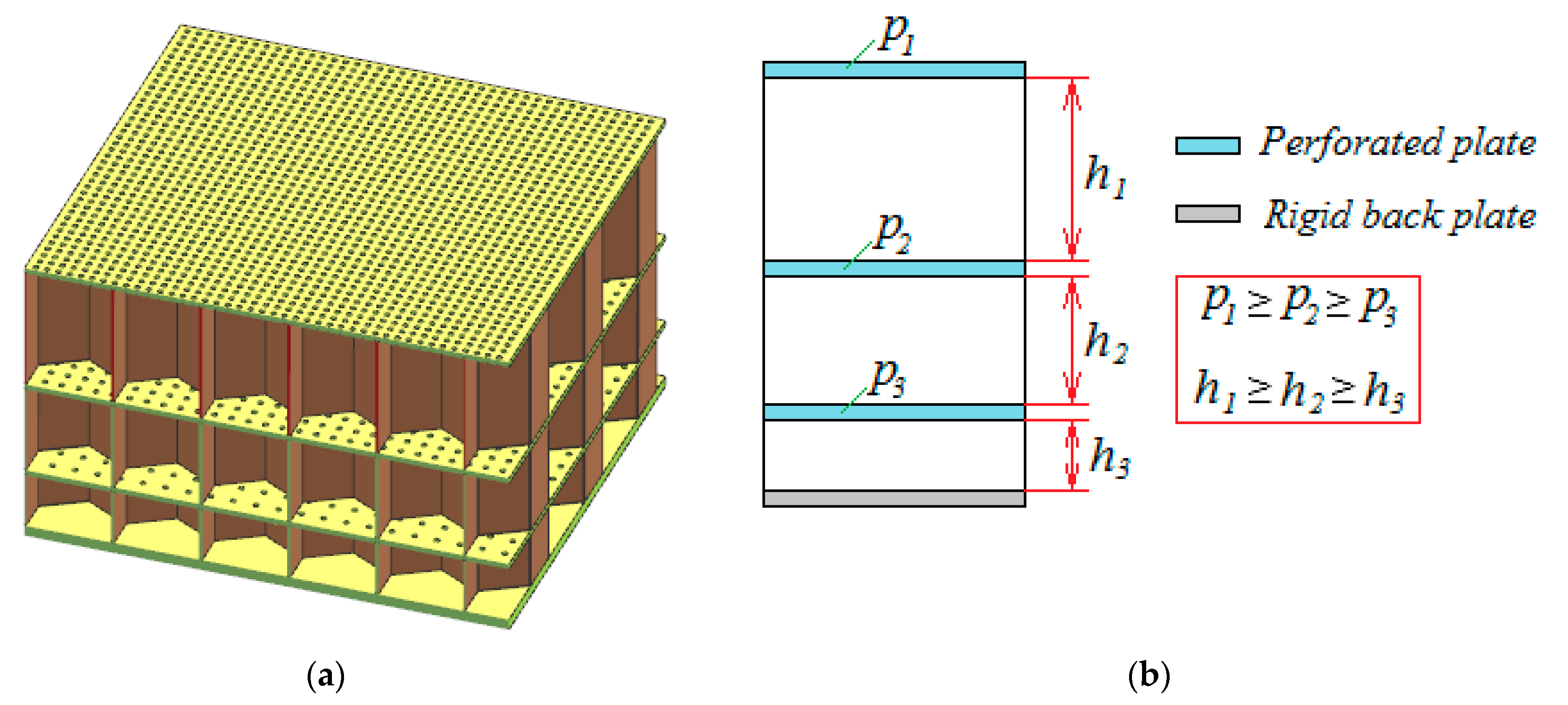
It is well known that the main source of noise in a modern aircraft bypass engine is a fan. To reduce fan noise, the air intake ducts and the bypass ducts are treated with locally reacting acoustic liners, which are resonators of various shapes, covered with thin perforated sheets (Figure 1a). The fundamental characteristic of the liner is an acoustic impedance. It is a complex value that depends on the geometric parameters of the liner (perforation degree, the resonator height, thickness of the perforated sheet) and on the specific external conditions, which primarily include a high level of sound pressure and the presence of a grazing flow in the duct. During the aircraft noise certification, measurements are carried out at three reference points on the ground corresponding to the take-off, landing and flyover. Thus, the frequency range of the fan noise turns out to be very wide (from low frequencies on landing to high frequencies on take-off, taking into account the fact that the maximum contribution can be made by harmonics above the first). To be able to tune the acoustic liner to the optimal impedance (the impedance that provides the maximum noise reduction in the far field) in a wide frequency range, the acoustic liner is made multilayered. Typically, the acoustic liner contains no more than three layers due to the increase in the dimensions and mass of the liner, which is critical for an aircraft. In a multilayer liner, the height of the layers and the perforation degree decrease with distance from the front surface towards the rigid backing (Figure 1b).

There are a number of methods for determining the impedance of the acoustic liners based on measuring the sound field in the duct of the experimental installation. In particular, one can note such standardized methods as the method using standing wave ratio [1] and the transfer function method [2] proposed in [3,4]. Some methods have been developed to determine the impedance, taking into account the influence of the grazing flow in the duct. The most popular among them is the impedance eduction method, which can be found in detail in [5,6,7,8]. Other methods of impedance determination can also be noted based on measurements of an acoustic liner sample in a grazing flow impedance tube: the direct method with determination of the axial wave numbers by Prony’s method [9,10]; single-mode method [10,11]; three-zone method [12]; 4-microphone method [13,14]; 6-microphone method [15]; and analytical method taking into account the passage of sound modes through the impedance transition [16].

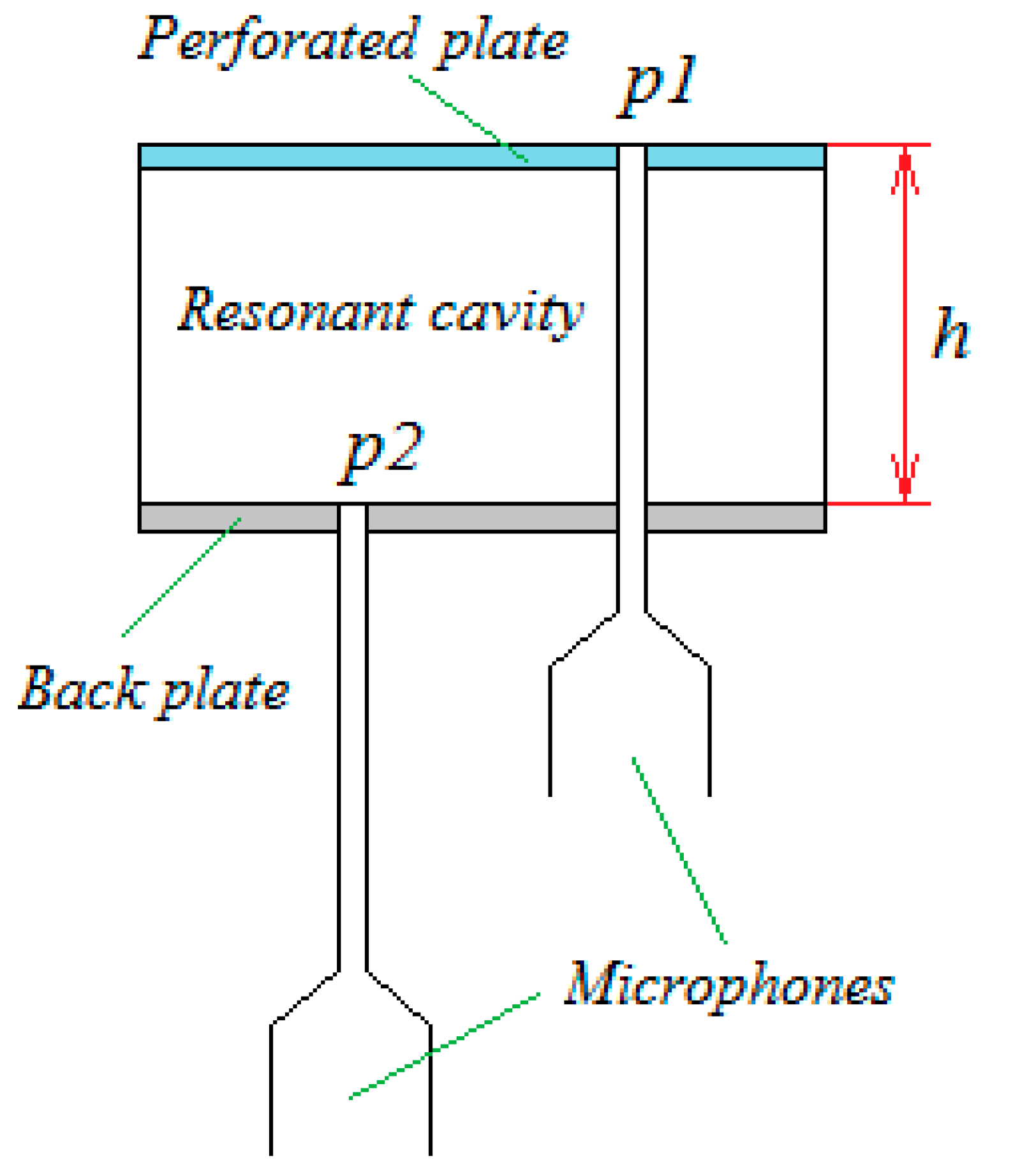
Another method for determination of acoustic liner impedance both on normal incidence impedance tube and on grazing flow impedance tube is the Dean’s method [17]. In contrast to the methods mentioned above, in this approach, microphones are installed in the walls of the resonator’s cover and backing. The method consists of measuring the sound pressure p1 on the front surface of the resonator and the sound pressure p2 on the resonator backing (Figure 2) with subsequent calculation of the normalized impedance by the formula:

$$Z=-i\frac{p1}{p2}{e}^{i\phi }\frac{1}{sin(kh)},$$

(1)

where φ is a phase between acoustic pressures p1 and p2; k is a freespace wave number; h is a distance between the front surface and the resonator backing; i is an imaginary unit.

It is noteworthy that this method makes it possible to determine the impedance of an acoustic liner installed directly on an aircraft engine [18]. This factor is extremely important from the point of view of verifying the methods for tuning the acoustic liner to the optimal impedance. However, Dean’s method also has disadvantages. Firstly, after mounting the measuring probes into the resonator, its integrity is violated, which can lead to some distortion of the acoustic characteristics of the resonator and it may be necessary to restore the integrity of the liner sample if further impedance measurements are carried out by other methods. Secondly, the implementation of this method is very laborious, which is associated with precise installation of the probes into the resonator (especially in the case of multilayer liner) and with the use of additional devices for rigid fixation of the microphones. Thirdly, as proved by calculations in [19], Dean’s method determines the impedance of only one resonator; therefore, to obtain the impedance of the whole liner, it is required to carry out many measurements at different points of the liner.

The disadvantages listed above relate to the implementation of Dean’s method in a full-scale experiment, but they are absent when the experiment is replaced by numerical simulation. However, the method has another drawback, which we will focus on in this study. It lies in the fact that Formula (1) was derived under the assumption that only plane waves propagate in the resonant cavity. This assumption is valid for most cases, since the non-uniformity of the pressure field caused by the passage of a sound wave through a perforated plate is observed only near orifices and then, with an increase in the depth of the resonator, the wave becomes plane. In addition to the depth of the resonator, the uniformity of the sound field over the cross section is affected by the perforation degree of the liner: the higher the perforation degree, the faster the wave becomes plane along the cavity depth. It is also worth noting that the non-uniformity of the pressure field at the resonator backing increases as frequency increases.

In the case of low height and low perforation degree of a resonator, another geometric parameter appears that can affect the non-uniformity of the sound field at the resonator backing—this is the position of the orifices in the resonator cover. This parameter does not apply to the geometric characteristics of the acoustic liner, since in industrial production the space between the orifices remains constant (Figure 1); however, in this case, the orifices can fall on the ribs of the resonator walls. This leads to the appearance of uncharacteristic narrowband peaks in the impedance spectra, which can be seen in [20]. In addition, a different number of orifices can fall on a different number of resonator cells, so it is necessary to carry out measurements in different resonators, since just one measurement may provide us inaccurate values of the liner impedance. To avoid the mentioned problems in scientific research, orifices in liner samples are often spaced unequally so that the same number of orifices fall on each resonator, providing a given perforation degree for both an individual resonator and the whole liner sample [21].

Thus, the objectives of the study are as follows:

• evaluation of the effect of the orifice arrangement in the resonator cover at low height and low perforation degree of the resonator on the impedance determined by the Dean’s Formula (1);
• elimination of the inaccuracy in determining the impedance associated with a more complex modal structure of the sound field at the resonator backing.

The article is structured as follows: Section 2 contains a detailed description of the numerical simulation of the plane wave incidence onto the resonator to obtain the sound field on the resonator backing at many points, which is difficult to provide in a natural experiment. Section 3 presents the numerical results of impedance determined by normal Dean’s formula for different orifice arrangements based on data obtained in numerical simulation. Section 4 considers the determination of the resonator impedance by Dean’s method, taking into account the complex modal structure of the sound field on the resonator backing (this is a new scientific result). Section 5 presents the concise results regarding numerical simulation, modal analysis and impedance analysis, followed by Section 6, which concludes the manuscript.

2. Numerical Simulation of the Physical Process in a Resonator under the Incidence of Plane Waves

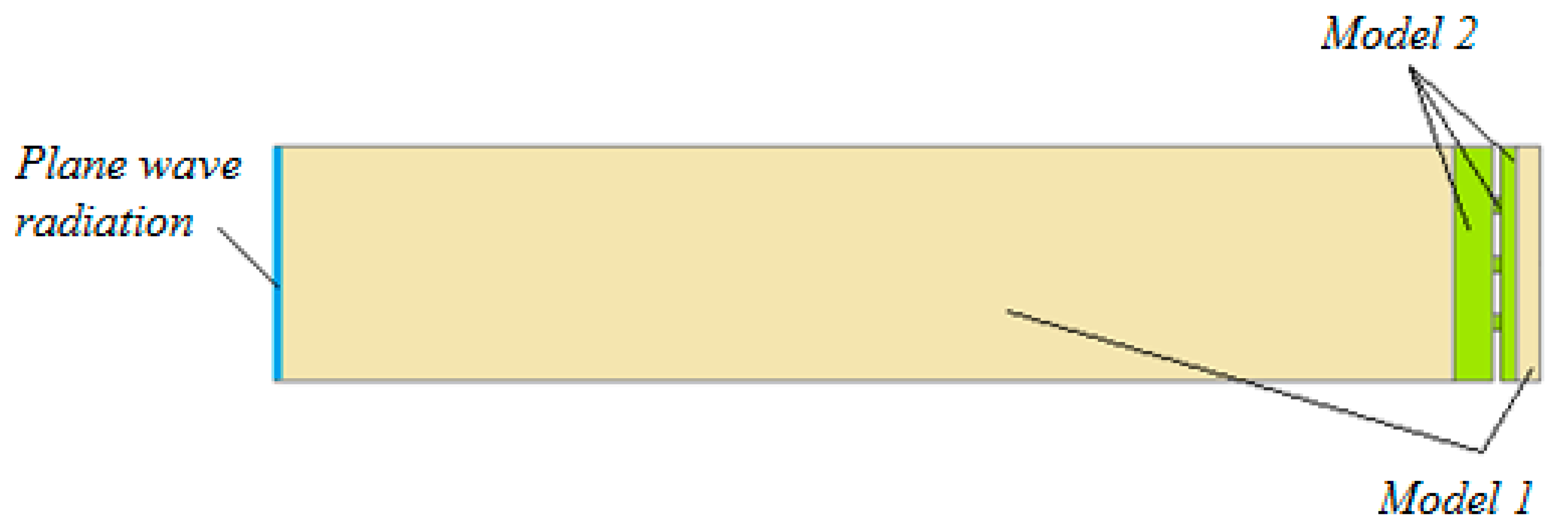
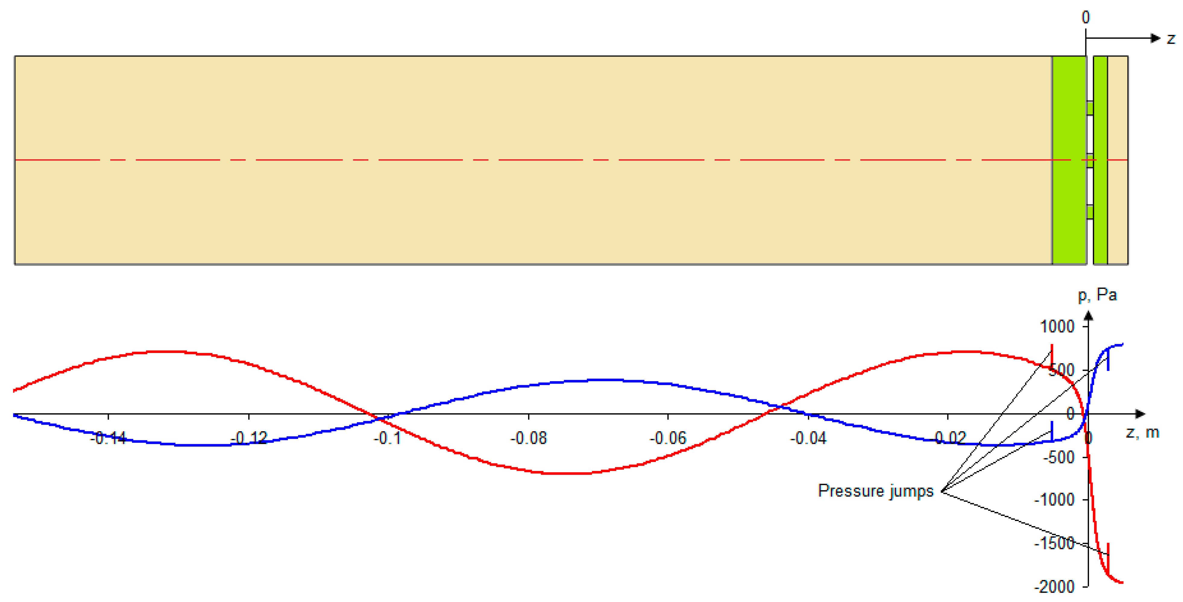
To obtain the values of the acoustic pressure at the resonator cover and resonator backing at different orifice arrangements, a number of computations are carried out. The computations consist of the numerical simulation of the physical process in a resonator installed in a normal incidence impedance tube. A three-dimensional geometric model of the computational domain is the internal volume of the cylindrical resonator, where acoustic processes occur, attached to the tube 150 mm long. On the other side of the tube, plane wave radiation is applied (Figure 3). The inner diameter of the impedance tube is 30 mm; therefore, only a plane wave propagates in the frequency range of interests 500–6000 Hz.

The geometric characteristics of the cylindrical resonator are presented in

Table 1. Geometry of the resonator under consideration.

Characteristic	Symbol	Value
Inner diameter of the resonator, mm	D	30
Height of the resonant cavity, mm	h	5
Perforated plate thickness, mm	t	1
Orifice diameter, mm	d	2
Number of the orifices	n	7
Perforation degree, %	p	3.1

.

To save computational resources, the computational domain is divided into two subdomains. The first subdomain, in which only acoustic wave propagation occurs at a given frequency, occupies most of the computational domain and acoustic processes in it are described by the Helmholtz equation (hereinafter referred to as Model 1):

$$\Delta p+k^{2}p=0,$$

(2)

where p is an acoustic pressure; k is a freespace wave number.

The second subdomain is located in the orifices of the resonator cover and near the orifices on the side of the tube and the cavity of the resonator. This subdomain was created to simulate the loss of acoustic energy due to friction of particles of the medium on the walls. The physical processes occurring in this subdomain are described (hereinafter referred to as Model 2) by:

$$\begin{array}{cc}-\mathrm{continuity}\mathrm{equation}\hspace{1em}\hspace{1em}\hspace{1em}\hspace{1em}\hspace{1em}\hspace{1em}\hspace{1em}\hfill & \hfill i\omega \rho +\nabla \cdot ({\rho }_0\mathbf{u})=0,\hspace{1em}\hspace{1em}\hspace{1em}\hspace{1em}\hspace{1em}\hspace{1em}\hspace{1em}\hfill \end{array}$$

(3)

$$\begin{array}{cc}-\mathrm{momentum}\mathrm{equation}\hspace{1em}\hspace{1em}\hspace{1em}\hspace{1em}\hspace{1em}\hspace{1em}\hspace{1em}\hspace{1em}\hfill & \hfill i\omega {\rho }_0\mathbf{u}=\nabla \cdot \mathsf{\sigma },\hspace{1em}\hspace{1em}\hspace{1em}\hspace{1em}\hspace{1em}\hspace{1em}\hspace{1em}\hspace{1em}\hfill \end{array}$$

(4)

$$\begin{array}{cc}-\mathrm{energy}\mathrm{equation}\hspace{1em}\hspace{1em}\hfill & \hfill {\rho }_0{C}_{\mathrm{p}}\left(i\omega T+\mathbf{u}\cdot \nabla T_0\right)-{\alpha }_{\mathrm{p}}{T}_0\left(i\omega p+\mathbf{u}\cdot \nabla p_0\right)=\nabla \cdot (kT),\hfill \end{array}$$

(5)

$$\begin{array}{cc}-\mathrm{equation}\mathrm{of}\mathrm{state}\hspace{1em}\hspace{1em}\hspace{1em}\hspace{1em}\hspace{1em}\hspace{1em}\hspace{1em}\hspace{1em} \hfill & \hfill \rho ={\rho }_0({\beta }_{\mathrm{T}}p-{\alpha }_{\mathrm{p}}T).\hspace{1em}\hspace{1em}\hspace{1em}\hspace{1em}\hspace{1em}\hspace{1em}\hspace{1em}\hfill \end{array}$$

(6)

Here, $\mathbf{\sigma }=-p\mathbf{I}+\mu \left(\nabla \mathbf{u}+{\left(\nabla \mathbf{u}\right)}^{\mathrm{T}}\right)-\left(\frac{2}{3}\mu -{\mu }_{\mathrm{B}}\right)\left(\nabla \cdot \mathbf{u}\right)\mathbf{I}$ is the stress tensor; $\mathbf{u}={\left\{\begin{array}{ccc}{u}_x& u_y& u_z\end{array}\right\}}^{\mathrm{T}}$ is the acoustic velocity field; $\rho$ is the acoustic density; $T$ is the acoustic temperature; $\omega$ is the angular frequency; $\mathbf{I}$ is the identity tensor; $\mu$ is the dynamic viscosity; ${\mu }_{\mathrm{B}}$ is the bulk viscosity; $C_{\mathrm{p}}$ is the heat capacity at constant pressure; ${\alpha }_{\mathrm{p}}$ is the coefficient of thermal expansion; $k$ is the thermal conductivity; ${\beta }_{\mathrm{T}}$ is the isothermal compressibility. The subscript 0 refers to the parameters of the equilibrium state.

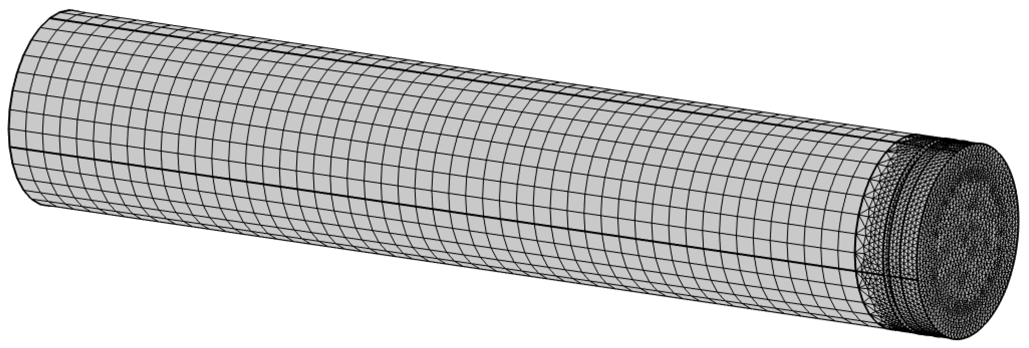
A slight expansion of the second subdomain from the orifices towards the tube and resonant cavity is made to provide a smoother transition of the finite element mesh from orifices with a small diameter to the large diameter of the tube and resonator (Figure 4). This configuration reduces the jump in the values of acoustic parameters at the boundary nodes connecting the subdomains for Model 1 and Model 2. Figure 5 shows an example of the acoustic pressure distribution taken along the symmetry axis of the geometric model (coordinate z = 0 corresponds to the front surface of the resonator; z-axis is directed towards the resonator backing). It can be seen that, despite the jumps at the boundary nodes, the acoustic pressure corresponds to the general trend of a smooth change in pressure along the axis.

Equations (2)–(6) are solved by the finite element method in the COMSOL Multiphysics software. For Model 1, a quadratic Lagrange finite element is used. In Model 2, pressure and temperature are approximated by a quadratic Lagrange finite element and velocity is approximated by a cubic Lagrange finite element. The maximum finite element size for subdomain 1 is chosen to provide 20 elements per wavelength at 6000 Hz; for subdomain 2, the sizes of the elements are even smaller. A boundary layer is applied to the walls of the orifices. The thickness of the wall layer element is set to the viscous penetration depth ${\delta }_{visc}=\sqrt{2\mu /\omega {\rho }_0}$. Air is used as the working medium in the numerical simulation. Computations are carried out at normal environmental conditions in the frequency range 500–6000 Hz with a step of 100 Hz. The basic parameters of the numerical simulation are presented in

Table 2. Basic parameters of the numerical simulation.

Characteristic	Symbol	Value
Static pressure, Pa	$p_0$	101,325
Static temperature, C	$T_0$	20
Maximum element size, mm	${\delta }_{\max }$	2.8
Minimum element size, mm	${\delta }_{\min }$	0.028

.

3. Calculation of Resonator Impedance Using the Normal Dean’s Formula

The numerical simulation considered in Section 2 was performed for various arrangements of orifices in the resonator cover (Figure 6). The red color dot indicates the point where the acoustic pressure is recorded in the numerical simulation to use it as the pressure p1 when calculating the impedance using Formula (1). The pressure p2 is recorded at the resonator backing at the point exactly under the red dot shown in Figure 6.

Figure 7 demonstrates the curves of the normalized impedance obtained by Formula (1) for different orifice arrangements in the resonator cover. It can be seen that at high frequencies, completely different dependencies of the impedance on frequency are obtained. Moreover, their discrepancy is already noticeable at a frequency of 3000 Hz, where the ratio of the wavelength to the resonator height is still quite large. This result is obviously due to the fact that the acoustic pressure field at the resonator backing is not uniform (the incident wave is out-of-plane). In addition, different orifice arrangements lead to different irregularities of sound pressure at the resonator backing. To confirm this statement, it is proposed to carry out a modal analysis of the sound field at the resonator backing for all three variants of the orifice arrangement. It allows us to extract zeroth order mode and use it in Formula (1) instead of the acoustic pressure p2.

4. Impedance Determination by the Modified Dean’s Formula

The modal analysis of the sound field at the resonator backing consists of determination of the amplitude coefficients of the acoustic modes. It is based on minimizing the residual function, which is the sum difference of squares of absolute values of acoustic pressure $P^{\mathrm{e}}$ obtained in numerical simulation and theoretical acoustic pressure $P^{\mathrm{t}}$:

$$\mathrm{\Phi }={\displaystyle \sum _{k=1}^K{\left|P_k^{\mathrm{e}}-P_k^{\mathrm{t}}\right|}^2},$$

(7)

where k is an index of a point at the resonator backing where acoustic pressure is determined; K is a number of points at the resonator backing.

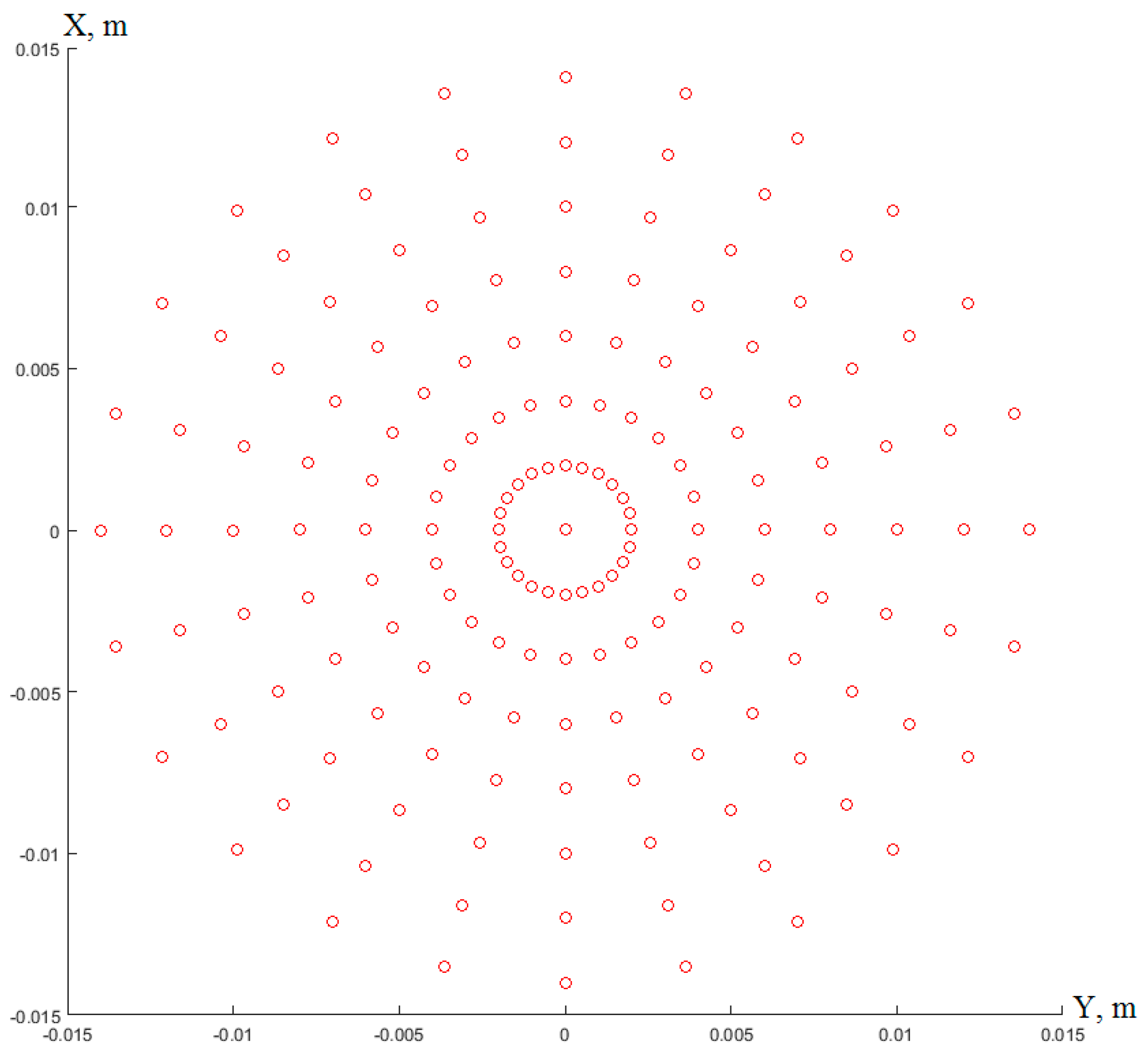
The array of points at the resonator backing for recording acoustic pressure $P^{\mathrm{e}}$ in numerical simulation is shown in Figure 8.

The theoretical value of the acoustic pressure at circular cross section of a cylindrical duct is the sum of the acoustic modes:

$$P_k^{\mathrm{t}}={\displaystyle \sum _{m=-M}^M{\displaystyle \sum _{n=0}^N{C}_{mn}{W}_{mn}{J}_{\left|m\right|}(k_{rmn}{r}_k)e^{im{\theta }_k}}},$$

(8)

where m, n are the circumferential and radial orders; M, N are the limits of circumferential and radial orders; $C_{mn}$ is the amplitude mode coefficient; $J_{\left|m\right|}$ is the Bessel function of order m; $k_{rmn}={\lambda }_{mn}/R$ is the radial wave number; ${\lambda }_{mn}$ is n-th root of equation ${J^{\prime }}_{\left|m\right|}(x)=0$; $R$ is the radius of cylindrical cavity; $r_k$, ${\theta }_k$ is the radial and angular coordinate of k-th point at resonator backing. The normalization factor is given by:

$$W_{mn}=\{\begin{array}{cc}1& \mathrm{for} k_{rmn}=0\left(\mathrm{plane}\mathrm{wave}\right)\hfill \\ {\left[\left(1-{\left(\frac{m}{k_{rmn}R}\right)}^2\right){\left(J_{\left|m\right|}(k_{rmn}R)\right)}^2\right]}^{-\frac{1}{2}}& \mathrm{for} k_{rmn}\ne 0\hfill \end{array}$$

The minimization of residual function (7) is performed by the conjugate gradient method:

$${\left\{C\right\}}_{j+1}={\left\{C\right\}}_j-h_j\cdot {\left\{S\right\}}_j,$$

where $\left\{C\right\}$ is a column vector consisting of the amplitude coefficients of the modes $C_{mn}$ from Formula (8); j is iteration index; ${\left\{S\right\}}_j=\nabla {\mathrm{\Phi }}_j+b_{j-1}\cdot \nabla {\mathrm{\Phi }}_{j-1}$; $b_{j-1}={\Vert \nabla {\mathrm{\Phi }}_j\Vert }^2/{\Vert \nabla {\mathrm{\Phi }}_{j-1}\Vert }^2$; $\nabla \mathrm{\Phi }={\left\{\begin{array}{cccc}\frac{\partial \mathrm{\Phi }}{\partial C_1},& \frac{\partial \mathrm{\Phi }}{\partial C_2},& \cdots ,& \frac{\partial \mathrm{\Phi }}{\partial C_{(2M+1)(N+1)}}\end{array}\right\}}^{\mathrm{T}}$.

From the modal analysis of the sound field, we take the amplitude coefficient of the zeroth order mode $C_{00}$ corresponding to the acoustic pressure that would be at the resonator backing if only a plane wave incidences (for the zeroth order mode, the other multipliers in expression (8) are equal to unity) and substitute $C_{00}$ in Formula (1) instead of the pressure p2:

$$Z=-i\frac{p1}{C_{00}}{e}^{i\phi }\frac{1}{sin(kh)}.$$

(9)

Hereinafter, this formula is referred to as the modified Dean’s formula for calculating the resonator impedance.

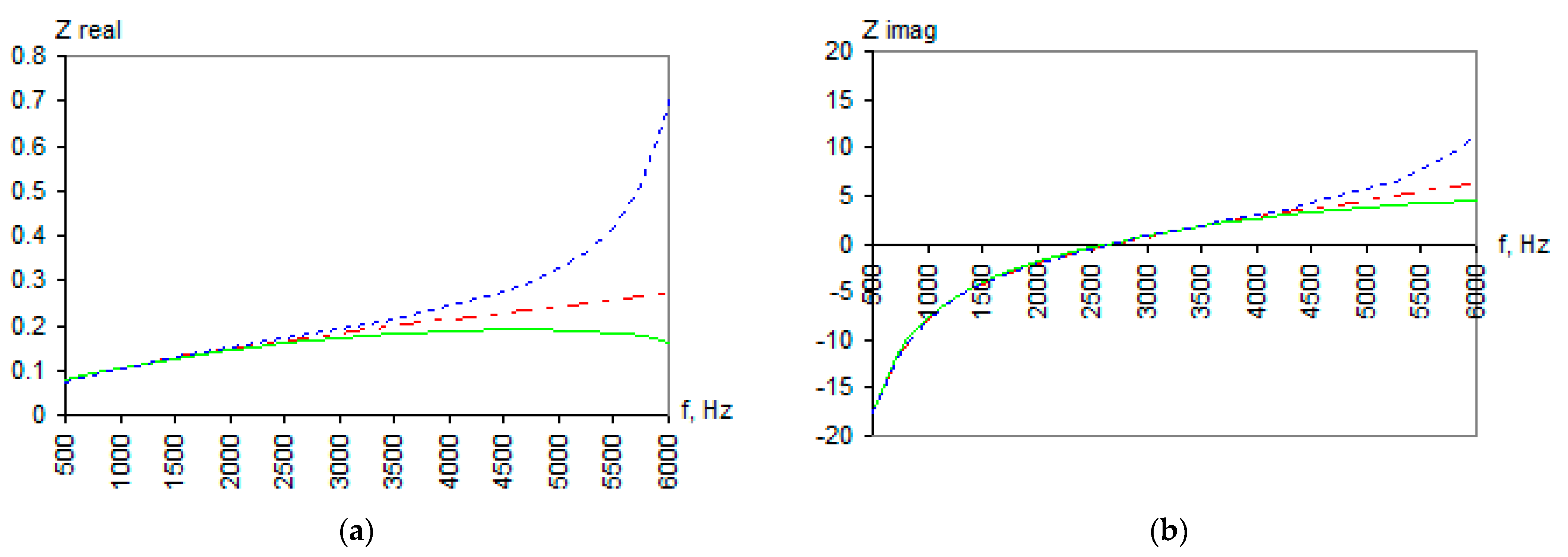
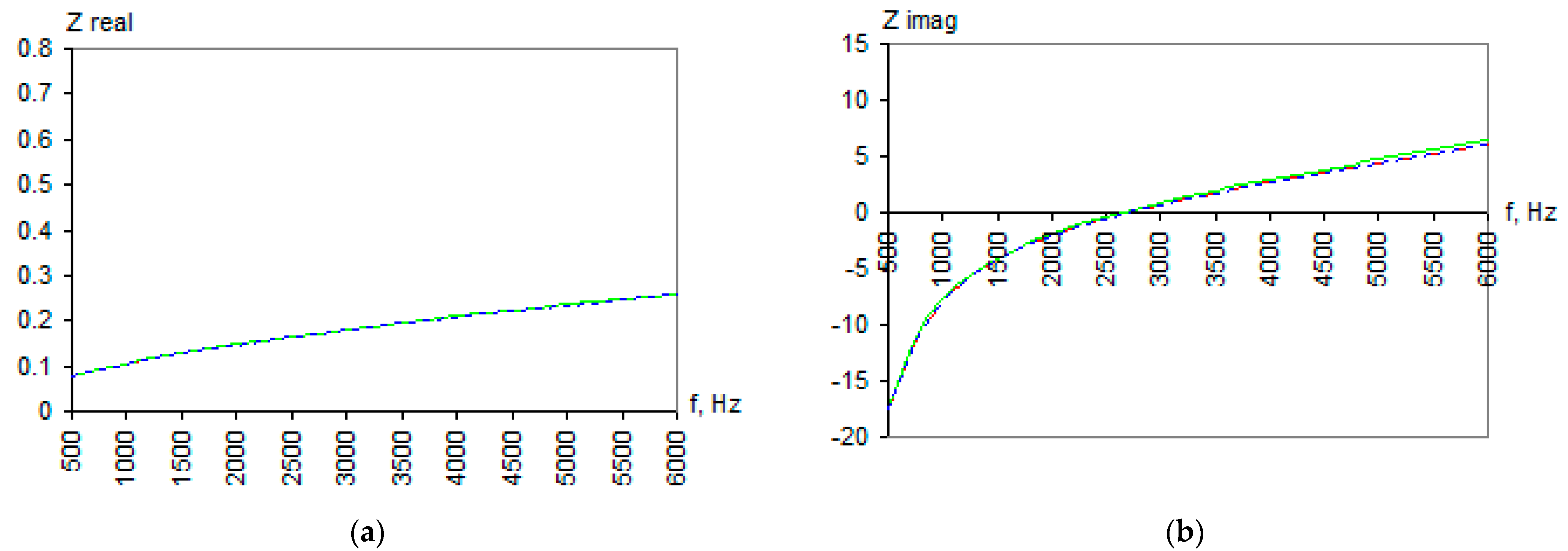
Figure 9 shows the results of impedance calculations according to the Formula (9). It is clearly seen that the impedance for all variants of the orifice arrangement fall within the same trend. Small deviations are associated with a limited number of modes in Formula (8), which are taken into account in modal analysis of the sound field at the resonator backing and also with the fact that the final value of the residual function (7) is not exactly zero.

Thus, we can conclude that the impedance determined by Formula (9) does not depend on the orifice arrangement in the resonator cover. In addition, we note that the impedance curves in Figure 9 coincide with those in Figure 7, determined by Formula (1) for the Variant 1 of the orifice arrangement, i.e., when the orifices are uniformly distributed in the resonator cover.

5. Discussion

As a result of the studies, it is revealed that the complex modal structure of the sound field at the resonator backing can greatly affect the impedance calculated by the normal Dean’s formula. Determination of the impedance taking into account the complex modal structure of the sound field in the resonator is proposed to perform in three steps: numerical simulation of the plane wave incidence onto the resonator; modal analysis of the sound field at the resonator backing; and calculation of the impedance by the modified Dean’s formula. Let us briefly discuss here the main points and results concerning each stage.

Numerical simulation of wave propagation in the impedance tube and in the most part of the resonator cavity can be performed based on the Helmholtz equation. For more correct modeling of acoustic energy dissipation in the orifices and their vicinity, numerical simulation is performed based on linearized equations of continuity, momentum and energy and equation of state. Conducting this stage allows us to determine the sound pressure field at the resonator backing at a multitude of points, which is extremely difficult to realize in a natural experiment. The results of the numerical simulation for a resonator with a small height and a low perforation degree indicate that:

• the sound field at the resonator backing is non-uniform for different orifice arrangements;
• the sound pressure distribution at the resonator backing is different for different orifice arrangements.

The modal analysis of the sound field at the resonator backing consists of finding the amplitude coefficients of sound modes. This problem can be solved on the basis of minimization of the residual function between the theoretical and experimental (in our case the natural experiment replaced by numerical simulation) values of the sound field. The minimization procedure can be performed by any known method, for example, by the method of conjugate gradients. The results of the modal analysis are the following:

• the amplitude coefficients of the zeroth order mode have been determined;
• the amplitude coefficients of the zeroth order mode turn out to be almost the same for different orifice arrangements.

The resonator impedance is calculated using the modified Dean’s formula. The distinction between the modified Dean’s formula and the normal Dean’s formula is that the amplitude coefficient of the zeroth order mode is used instead of the acoustic pressure at the resonator backing. The results of the calculations show that:

• impedance does not depend on the orifice arrangement in the resonator cover;
• with a uniform orifice arrangement, the impedance is the same as the impedance determined by the normal Dean’s formula.

6. Conclusions

The conducted studies show that for a resonator with a low height and a small perforation degree, the position of the orifices in the resonator cover can significantly change the impedance in the high-frequency region if it is determined by the normal Dean’s formula. This result is associated with the uneven distribution of acoustic pressure at the resonator backing. To make the impedance independent of the orifice arrangement, the authors propose the modification of the Dean’s formula by using the amplitude coefficient of the zeroth order mode instead of the acoustic pressure at the resonator backing.

Thus, it can be assumed that to determine the impedance by the Dean’s method in full-scale tests, it is better to use acoustic liner samples with uniformly distributed orifices. This should make it possible to accurately determine the impedance of a resonator with a small height and perforation degree only from measurements of acoustic pressure in one point at the resonator backing, i.e., use the normal Dean’s formula, and do not perform modal decomposition, because the impedance values for these two cases are the same. Confirmation of this assumption requires the collection of the statistics (conducting studies on samples with different numbers of orifices and their arrangement), which should also include the implementation of a full-scale experiment on measuring the acoustic pressure at many points of the resonator backing in order to conduct a modal analysis of the sound field.