1. Introduction
Time series forecasting plays a crucial role in a wide variety of real-world applications, ranging from weather prediction to power system planning and operation to financial risk assessment [
1,
2,
3]. While the forecast horizon varies in real-world applications, many of them require a long-term forecast. This is challenging due to long-term dependencies, error propagation, and complex dynamics, which are difficult to model [
4]. Despite these challenges, the increasing demand for precise and reliable long-term forecasts has drawn attention to this area [
4,
5,
6].
Real-world time series data frequently display complex traits such as non-stationarity and non-normality, complicating the task of Long-Term Time Series Forecasting (LTSF) [
7]. Non-stationarity refers to the evolving nature of the data distribution over time. More precisely, it can be characterized as a violation of the Strict-Sense Stationarity condition, defined by the following equation:
where
is the Cumulative Distribution Function (CDF).
Seasonality, deterministic and stochastic trends, heteroscedasticity, and structural breaks are common types of non-stationarity usually observed in time series data. Furthermore, the data distribution can deviate significantly from a normal distribution, manifesting features such as fat tails or exhibiting conditions such as outliers or intermittency within the series [
7].
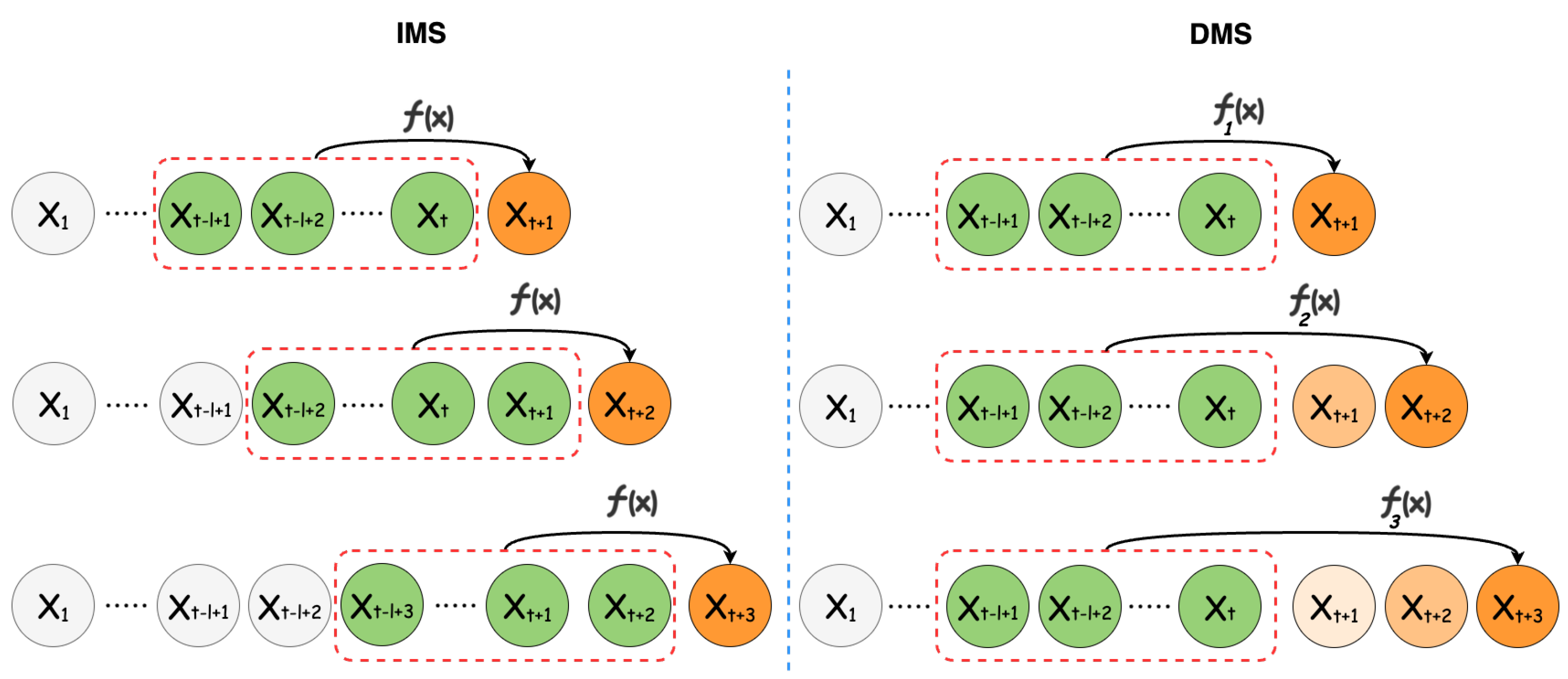
The LTSF problem can be addressed using two approaches [
8], illustrated in
Figure 1:
Iterative Multi-Step (IMS): In this approach, forecasts are made incrementally for each time step within the forecast horizon. Specifically, a single forecast is generated, after which, the look-back window is shifted forward by one time step to incorporate the newly created prediction. This process is then repeated iteratively.
Direct Multi-Step (DMS): Contrary to the IMS method, this method generates forecast values for the entire horizon in a single computational pass, thereby producing all the required forecasts simultaneously.
Each approach excels under specific conditions. For instance, the IMS method is particularly advantageous when dealing with shorter forecast horizons, where single-step accuracy is paramount. However, this technique is prone to error accumulation and typically requires a longer inference time compared to its counterpart. As a result, the DMS method is often the go-to choice for LTSF, offering a more-efficient and often more-reliable solution for extended forecast horizons [
6]. Forecasting can also be approached through univariate or multivariate methods. In the univariate approach, each time series is modeled and predicted independently, neglecting its interactions with others. On the contrary, the multivariate method accounts for the relationships among different varieties.
In today’s world, with the vast amounts of data available, there is a growing trend of using Machine Learning and Deep Learning for time series predictions. These advanced models outperform traditional statistical methods in both efficacy and accuracy. Many recent studies advocating deep neural network approaches for LTSF propose increasingly intricate networks, often more elaborate than previous ones, to address the challenges involved. However, these studies often overlook simple, but highly effective techniques, such as decomposing a time series into its constituents as a preprocessing step, as their focus is mainly on the forecasting model.
We advocate for a univariate DMS method to address the intrinsic challenges associated with the LTSF task. This approach employs a multiseasonal decomposition technique, known as the MSTL [
9], to break down the time series data into its foundational elements, namely the trend, various seasonal components, and residuals. Each component is then analyzed and predicted separately. Experiments with real-world and synthetic data demonstrated that the proposed method, Decompose & Conquer, outperformed state-of-the-art methods by a substantial margin. We attributed this improvement to the better choice of the decomposition method and to the handling of the extracted components separately. This approach and its name were inspired by the renowned divide-and-conquer algorithm design paradigm to overcome complexity.
The contributions of this paper can be summarized as follows:
We propose a novel forecasting approach that breaks down time series data into their fundamental components and addresses each component separately.
We assessed the model’s efficiency with real-world time series datasets from various fields, demonstrating the enhanced performance of the proposed method. We further show that the improvement over the state-of-the-art was statistically significant.
We designed and implemented a synthetic-data-generation process to further evaluate the effectiveness of the proposed model in the presence of different seasonal components.
2. Related Work
Data-driven approaches to time series forecasting offer several benefits, including flexibility, scalability, and robustness to noise, making them valuable tools for understanding and predicting complex systems. Existing data-driven time series forecasting methods can be broadly categorized into classical, Machine Learning, and Deep Learning models.
2.1. Classical Time Series Models
Classical time series forecasting models, such as the Autoregressive Integrated Moving Average (ARIMA) [
10,
11] and Exponential Smoothing [
12,
13], have long served as foundational pillars in the field of predictive analytics. These models excel at capturing linear relationships and identifying underlying patterns within the data, such as trends and seasonality. ARIMA, for instance, combines autoregressive, integrated, and moving average components to model a wide range of time series structures. Exponential Smoothing methods, such as Holt–Winters, focus on updating forecast estimates by considering the most-recent observations with exponentially decreasing weights for past data. These classical models lack the complexity to tackle some of the intricacies present in modern datasets, such as the non-stationarity of the underlying distribution and the non-linearity of temporal and spatial relationships.
2.2. Machine Learning Models
Machine-Learning-based time series forecasting models such as Random Forests [
14], Support Vector Machines [
15], and various types of neural networks have risen to prominence for their ability to handle complex, non-linear relationships within data. Unlike traditional statistical models, which are often constrained by assumptions such as linearity and stationarity, Machine Learning models offer a more-flexible and -adaptive framework to model time series data. However, they lack the interpretability that classical time series models provide.
2.3. Deep Neural Networks
With the rise of deep neural networks, Recurrent Neural Networks (RNNs) have emerged as specialized tools for handling sequential data. Within the RNN family, both LSTM [
16] and GRU [
17] utilize gated mechanisms to manage the flow of information, thus addressing challenges such as vanishing or exploding gradients. Attention-based RNNs [
18] employ temporal attention mechanisms to capture long-term relationships within the data. Nevertheless, recurrent models face limitations in parallelization and struggle with capturing long-term dependencies. Temporal Convolutional Networks (TCNs) [
19] present another efficient option for sequence-related tasks, but their capability is restricted by the receptive field of their kernels, making it difficult to grasp long-term dependencies.
2.4. Transformer-Based Architectures
The success of Transformer-based models [
20] in various AI tasks, such as natural language processing and computer vision, has led to increased interest in applying these techniques to time series forecasting. This success is largely attributed to the strength of the multi-head self-attention mechanism. The standard Transformer model, however, has certain shortcomings when applied to the LTSF problem, notably the quadratic time/memory complexity inherent in the original self-attention design and error accumulation from its autoregressive decoder. Informer [
21] seeks to mitigate these challenges by introducing an improved Transformer architecture with reduced complexity and adopting the DMS forecasting approach. Autoformer [
22] enhances data predictability by implementing a seasonal trend decomposition prior to each neural block, employing a moving average kernel on the input data to separate the trend–cyclical component. Building on Autoformer’s decomposition method, FEDformer [
5] introduces a frequency-enhanced architecture to capture time series features better. These Transformer-based models were used as baselines in this paper.
A recent study suggested that Transformer-based architectures may not be ideal for LTSF tasks [
6]. This is largely attributed to the permutation-invariant characteristic of the self-attention mechanism. Even with positional encoding, this mechanism does not completely preserve temporal information, which is crucial for attaining high accuracy in the LTSF task.
2.5. Time Series Decomposition
Time series decomposition concerns breaking time series data into components such as the trend, seasonality, and remainder. The decomposition methods provide clarity and structure to complex time series data, making it easier to model, interpret, and predict this kind of data.
In decomposition, an additive or multiplicative structure can be assumed for the forming components [
23]. Specifically, we can write:
for the additive method, where
is the value of the time series at
t and
,
, and
are its corresponding seasonality, trend, and remainder components at that time, respectively. Multiplicative methods can also be formulated as follows:
If the size of seasonal changes or deviations around the trend–cycle remain consistent regardless of the time series level, then the additive decomposition is suitable. On the other hand, if these variations correspond proportionally to the time series level, a multiplicative decomposition is better. Multiplicative decompositions are frequently used in economics [
23].
The classical way of time series decomposition consists of three main steps [
24]. First, the trend component is calculated using the moving average technique and removed from the data by subtraction or division for the additive or multiplicative cases. The seasonal component is then calculated simply by averaging the detrended data and then removed in a similar fashion. What is left is the remainder component. The studies [
6,
22] followed a similar approach by calculating the trend component, detrending the data, and treating the remainder as the second component. Although the use of this decomposition method has enormously improved previous results, showing the essence of decomposition for time series forecasting, there are still more-complex and -accurate decomposition methods to explore, such as X-13-ARIMA-SEATS [
25], X-12-ARIMA [
26], and Seasonal Trend decomposition using Loess (STL) [
27], to name a few.
While the aforementioned traditional methods are popular in many practical scenarios due to their reliability and effectiveness, they are often only suitable for time series with a singular seasonal pattern. Recently, however, approaches that accommodate multiseasonal trends have emerged, e.g., Seasonal Trend decomposition by Regression (STR) [
28], Fast-RobustSTL [
29], and forecasting-based models [
30].
One successful member of this family is Multiple Seasonal Trend decomposition using Loess (MSTL) [
9]. The MSTL is a versatile and robust method for decomposing a time series into its constituent components, especially when the data exhibit multiseasonal patterns. Building upon the classical Seasonal Trend decomposition procedure based on Loess (STL), the MSTL extends its capabilities to handle complex time series with more than one seasonal cycle. The method applies a sequence of STL decompositions, each tailored to a specific seasonal frequency, allowing for a more-subtle extraction of seasonal effects of different lengths.
3. Problem Formulation
Let be a time series of T observations, each having n dimensions. The goal of time series forecasting is that, given a look-back window of length l, ending at time t: , predict the next h steps of the time series as , where denotes the parameter of the forecasting model. We refer to a pair of look-back and forecast windows as a sample.
4. Methodology
In the first step, we employed the MSTL [
9] method to decompose time series data. The MSTL is an entirely self-operating additive algorithm for decomposing time series that exhibit several seasonal patterns. It is essentially an enhanced version of the traditional STL [
27] decomposition, wherein the STL technique is used iteratively to determine the various seasonal elements present within a time series. The MSTL modifies Equation (
2) to encompass several seasonal components within a time series as follows:
where
n is the number of seasonal components.
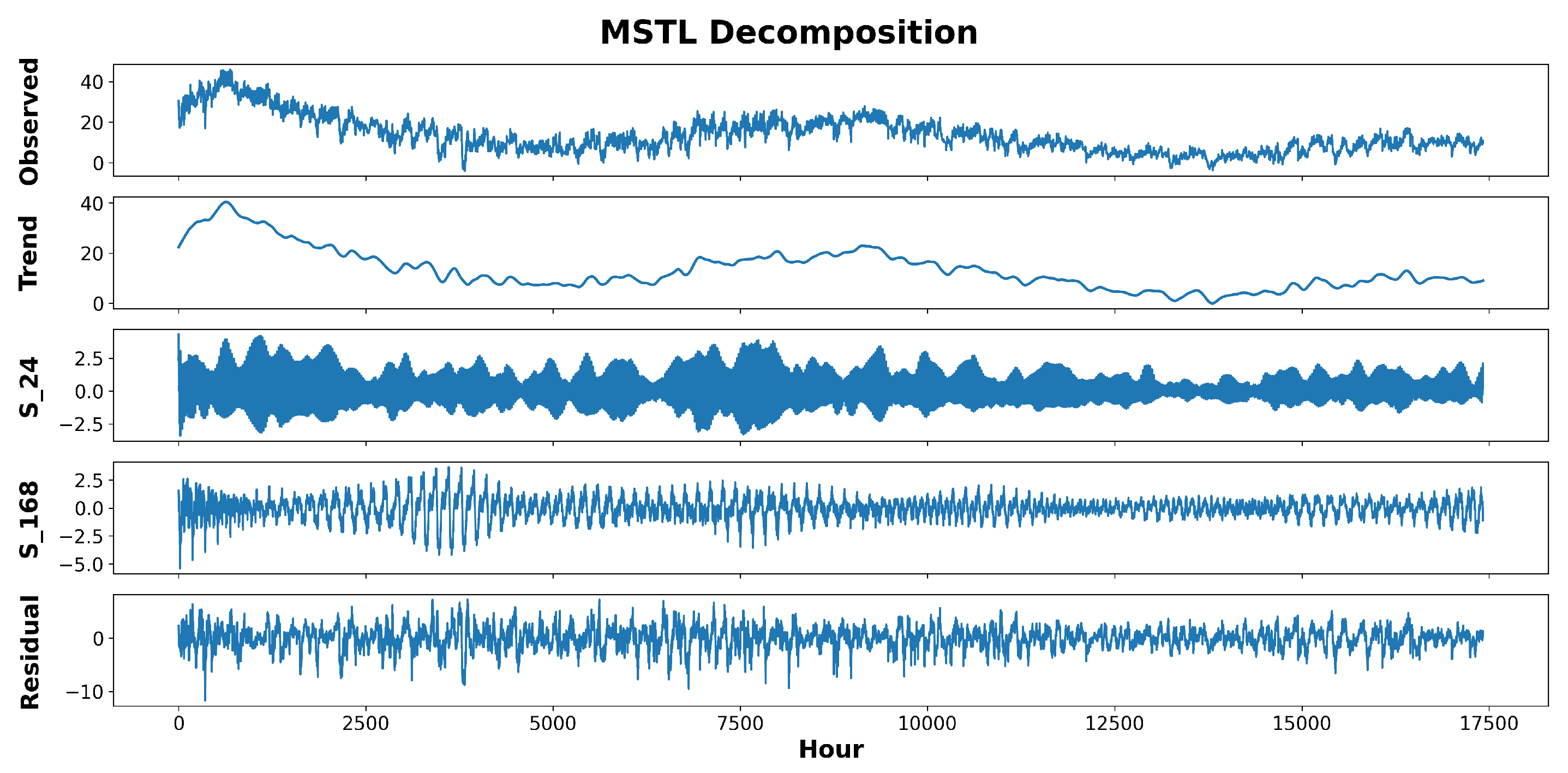
Figure 2 is an example of decomposing a time series into its components.
This method excels at deconstructing time series that exhibit multiseasonal trends. The decomposition results in various components that, when added up, recreate the original data. Subsequently, each component undergoes individual training and evaluation in a dedicated module.
To perform the decomposition, first, the whole dataset is split into training, validation, and test sets to prevent data leakage, and then, each set is decomposed independently using the MSTL decomposition method. The MSTL algorithm requires the length of seasonality periods as the input. To determine this, we can draw upon expert insights, i.e., visually inspecting the data by plotting or conducting a frequency domain analysis using the Fast Fourier Transform (FFT). The frequency domain analysis is performed by first detrending the dataset and transforming it to the frequency domain using the FFT, then picking up the dominant frequencies by looking at the power spectrum of the signal. For real datasets, we adopted the former approach, and for synthetic data, we followed the latter.
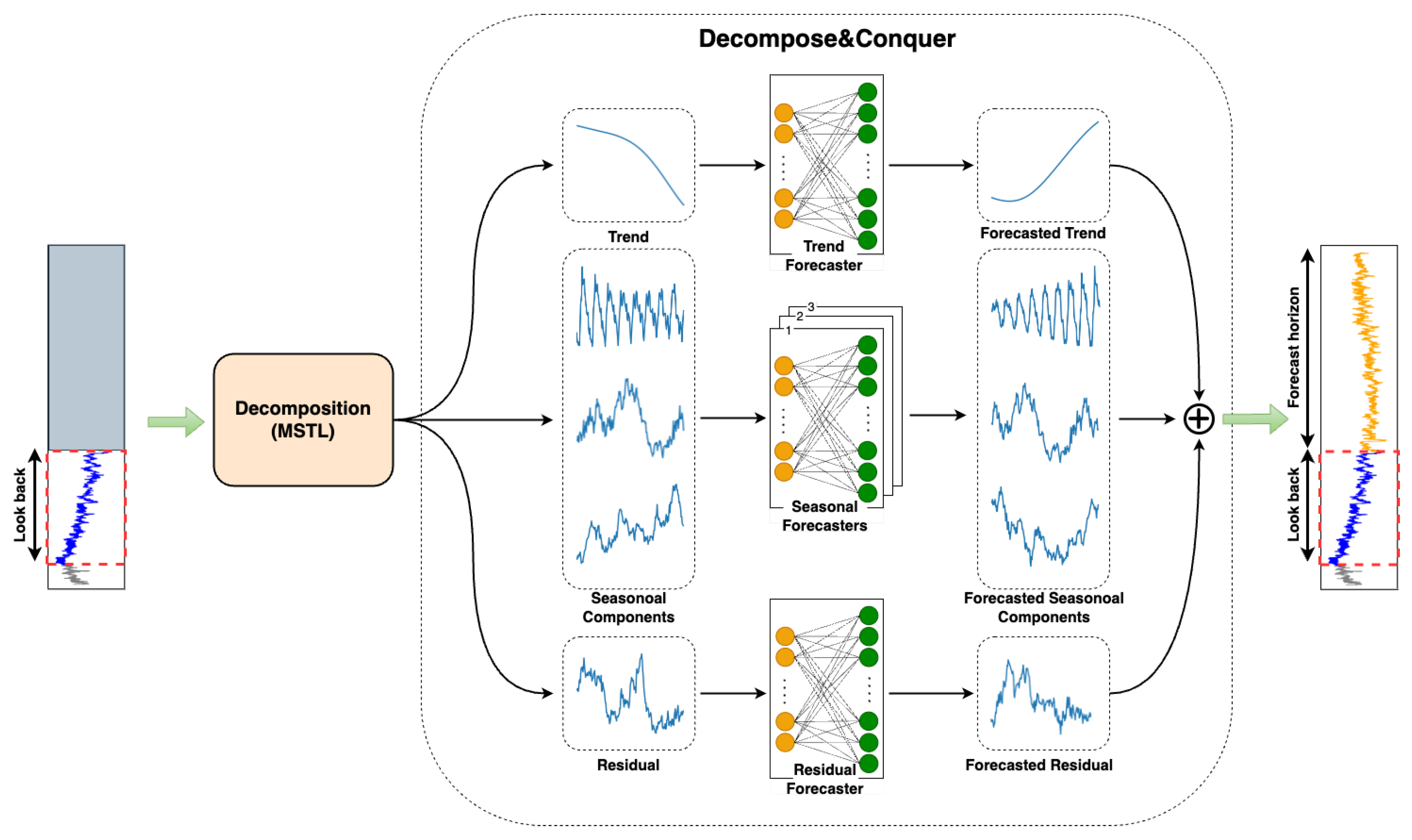
A solitary linear layer is sufficiently robust to model and forecast time series data provided it has been appropriately decomposed. Thus, we allocated a single linear layer for each component in this study. Upon receiving an input sequence, every linear layer independently generates the complete output sequence in a DMS fashion. These outputs are then aggregated to formulate the final forecast. The overall architecture of the proposed model is depicted in
Figure 3.
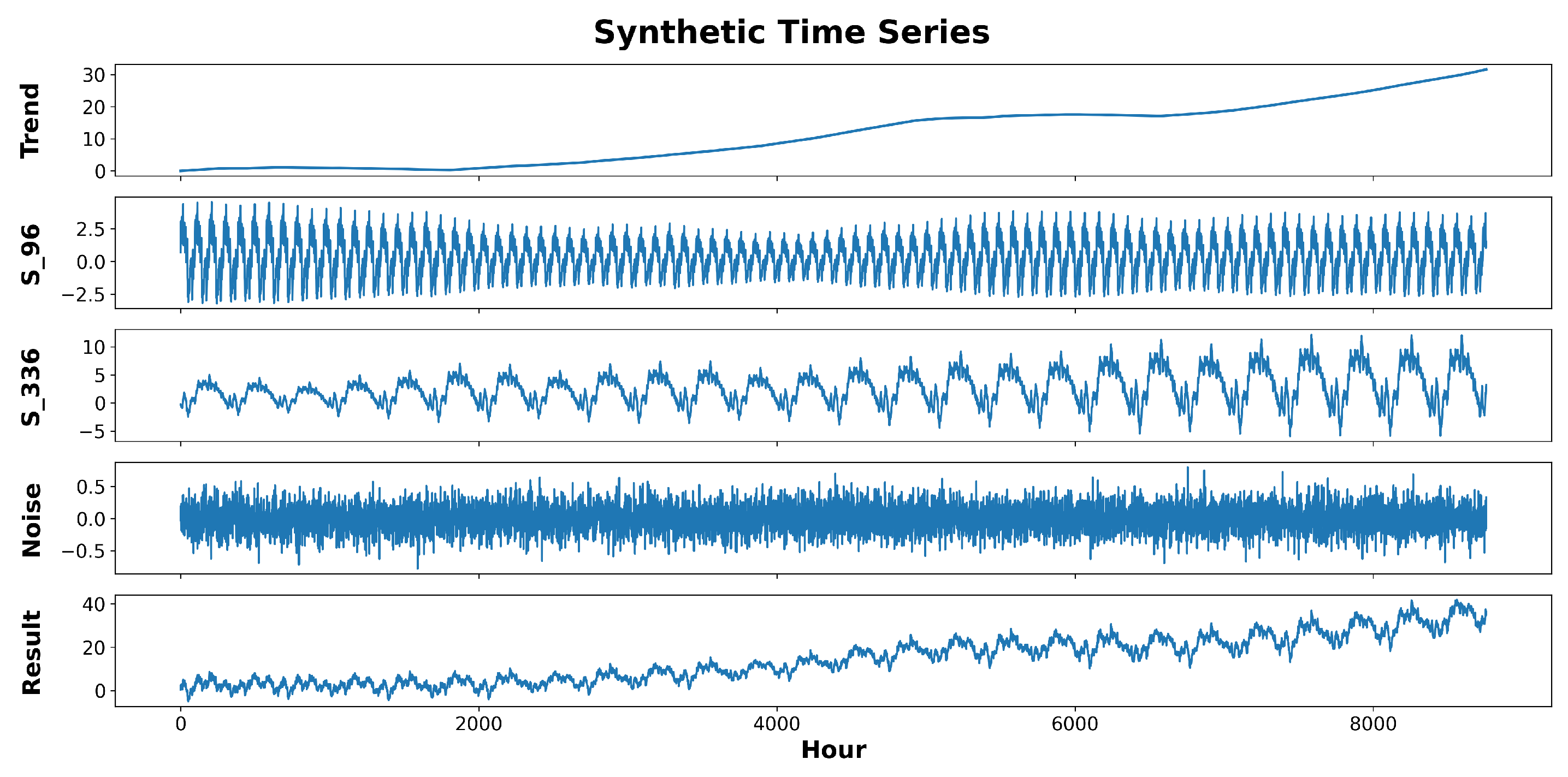
4.1. Synthetic Data Generation
To further validate the model’s performance, we generated some synthetic data by rendering random trend, seasonality, and noise components and adding them together to make a non-stationary time series. The generative process is expressed in the following equation:
where
,
, and
are the values of the trend, the
i-th seasonal component, and the noise at time
t, respectively.
To generate the trend component, we used a linear function of time with a slope of
and an intercept of
b. The slope,
, is an extension of the Gaussian random walk process, in which, at each time, we may take a Gaussian step with a probability of
p or stay in the same state with a probability of
:
Notice that is a Gaussian random variable itself because it is the sum of independent Gaussian random variables. The parameter p controls the frequency of potential changes in the trend component.
To generate each seasonal component, first, we generated one signal period using a Gaussian random walk process:
We then repeated the generated pattern (
S) for the requested length (
l). Each repetition is multiplied by the signal’s amplitude, coming from another Gaussian random process. The i-th repetition of the period is as follows.
Lastly, the noise component is generated using a white noise process. An example of a time series generated by the described process is depicted in
Figure 4.
4.2. Implementation Details
This study used the L2 loss paired with the ADAM [
31] optimization method. The learning rate was initialized at 1e-4, although it was subject to modification based on the ReduceLROnPlateau method. The batch size was configured as 32, and an early stoping criterion was established to stop the training after the evaluation measure (e.g., validation loss) did not improve for three consecutive checks. Each experiment was conducted five times, and the final results were obtained using the average metric value. The training/validation/testing split in all experiments was 2/3, 1/6, and 1/6. The Decompose & Conquer model was implemented using PyTorch [
32], wrapped with PyTorch Lightning [
33], and trained on a GeForce RTX 3090 24 GB GPU (by Nvidia).
5. Results
5.1. Datasets
The datasets used in this are described as follows.
Electricity (
https://archive.ics.uci.edu/ml/datasets/ElectricityLoadDiagrams20112014 (accessed on 9 December 2023)): Records the hourly electricity usage of 321 customers over a span of three years.
ETT [
21] datasets: Include the target value “oil temperature” along with six power load attributes. ETTm1 and ETTm2 data were noted every 15 min, while ETTh1 and ETTh2 data were logged hourly from 2016 to 2018.
Exchange [
34]: Features daily exchange rate data across eight countries from 1990 to 2010.
ILI (
https://pems.dot.ca.gov/ (accessed on 9 December 2023)): Documents the weekly ratio of patients with influenza-like symptoms to the overall patient count. This information was provided by the U.S. Centers for Disease Control and Prevention between 2002 and 2020.
Weather (
https://www.bgc-jena.mpg.de/wetter/ (accessed on 9 December 2023)): Represents a meteorological series with 21 weather metrics collected every ten minutes in 2020 from the Weather Station at the Max Planck Biogeochemistry Institute.
Traffic (
http://pems.dot.ca.gov (accessed on 9 December 2023)): Contains hourly data related to road occupancy rates from various sensors on freeways in the San Francisco Bay area. Provided by the California Department of Transportation, this dataset has 862 attributes and spans from 2016 to 2018. The main characteristics of all the datasets are summarized in
Table 1.
5.2. Evaluation Metrics
The forecasting errors were evaluated using two common metrics: the mean-squared error:
and the mean absolute error:
5.3. Baselines
For comparison, we included three effective Transformer models: Informer [
21], Autoformer [
22], and FEDformer [
5]. Two other baselines that have recently achieved state-of-the-art results are the NLinear and DLinear models [
6]. We also used Closest Repeat (Repeat Last) and Average Repeat (Repeat Avg.) as two straightforward baselines replicating the last and average in the look-back period, respectively. In this study, we did not compare the obtained results with classical models, such as ARIMA, SARIMA, etc., as their parameter selection procedure takes too long, which makes the training process extremely slow. Instead, we based our conclusions on the experimental results of these models from other studies [
21,
22], which demonstrated their poor performance on the LSTF task, and opted not to include them in this study directly.
5.4. Experimental Results on Real Data
Table 2 shows the results obtained using the proposed model and the baselines for all the real datasets included in this study.
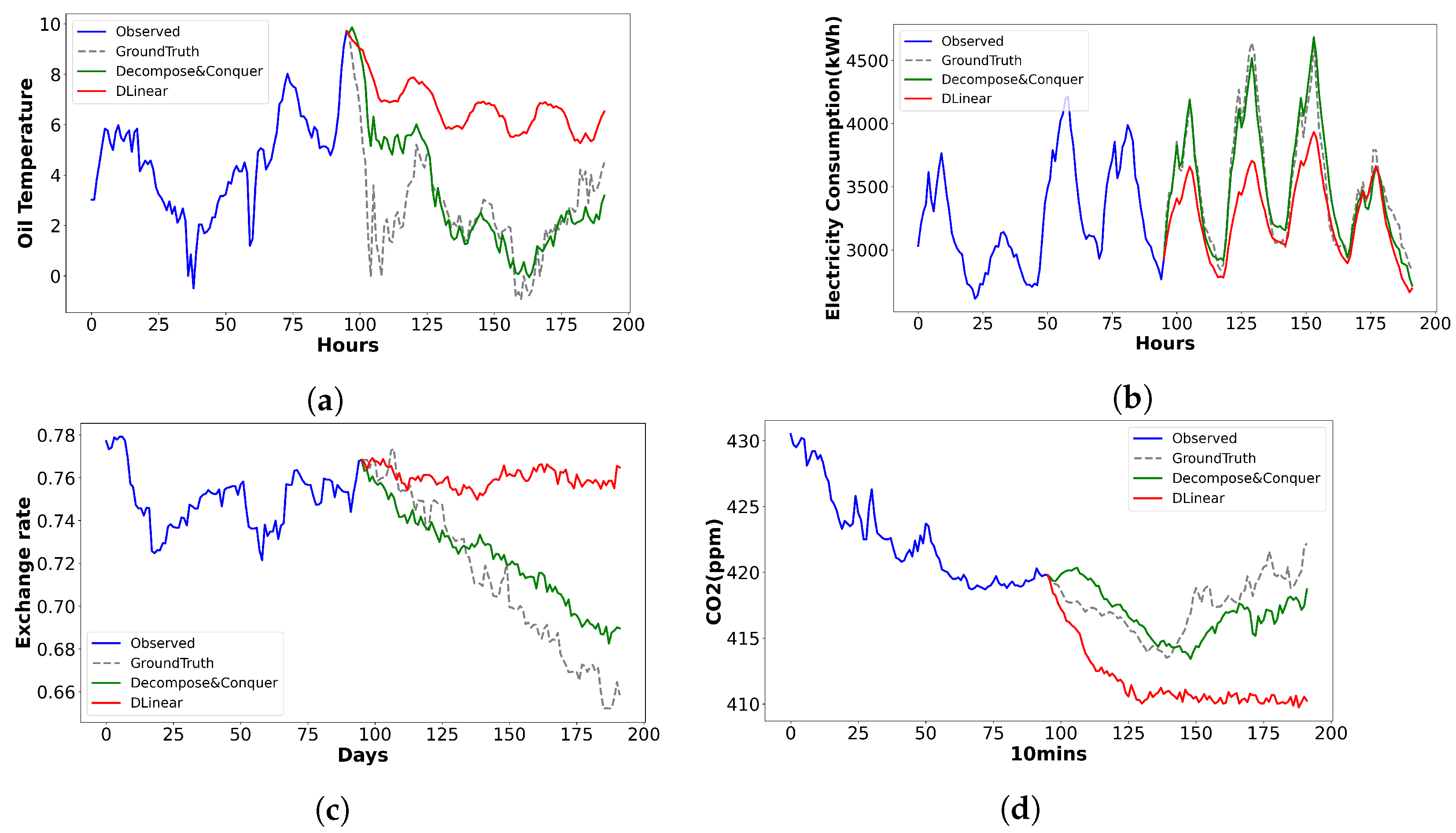
While a model’s performance is best compared using results from the entire dataset and a single instance is not conclusive proof of superiority, visualizing a few results can provide insights into the differences. To do this, we plot the forecasts made by the proposed model, Decompose & Conquer, with the second-best results achieved from other models using four arbitrarily selected datasets in
Figure 5.
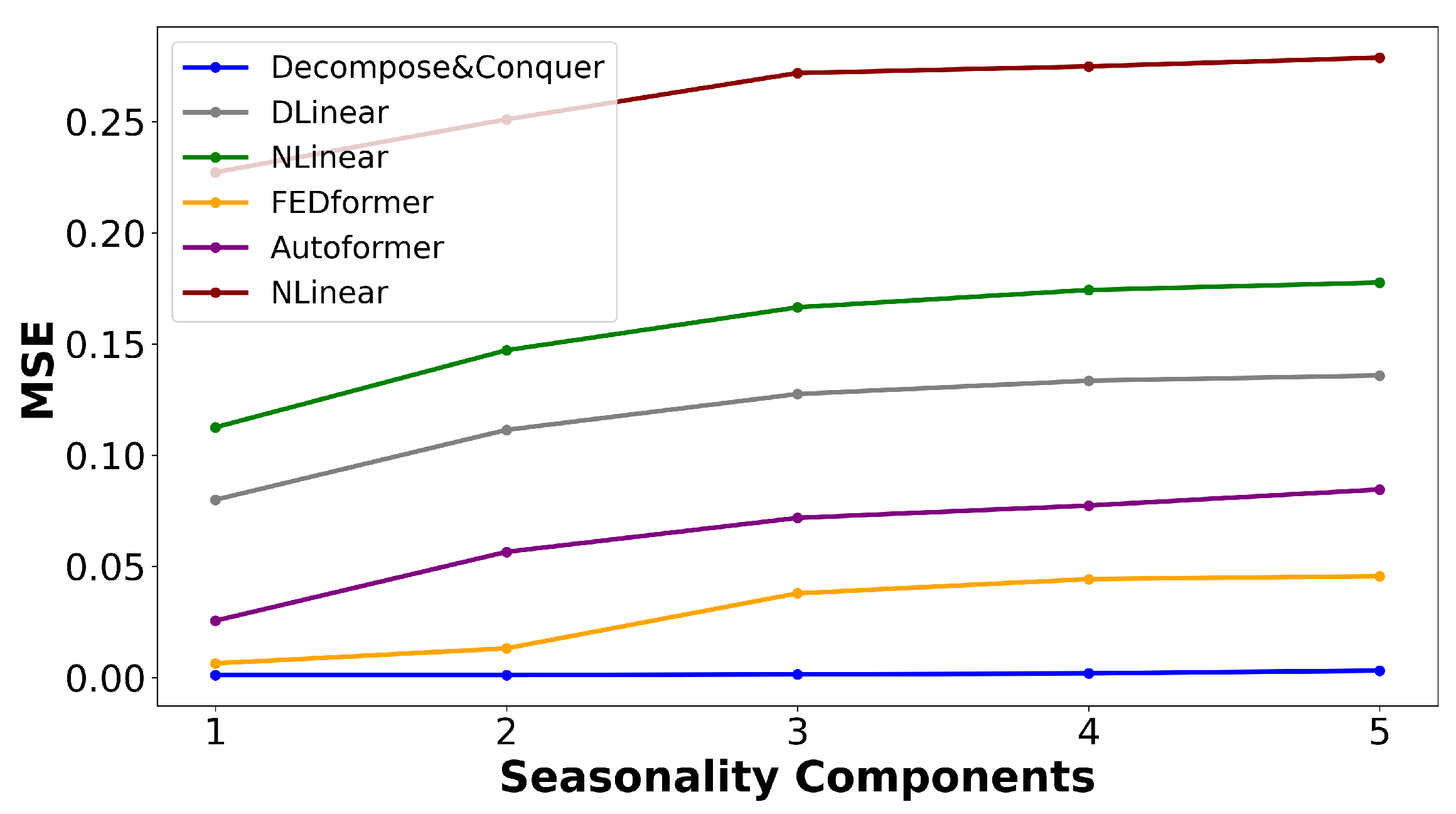
5.5. Experimental Results on Synthetic Data
Figure 6 illustrates the variations in the MSE as new seasonal components are introduced through the outlined data-generation process. This chart indicates that the proposed model not only delivered superior performance, but remained robust when additional seasonal components were added.
5.6. Statistical Tests
A straightforward method for deciding between two predictions is to opt for the one with the lower error or highest performance according to the evaluation metrics outlined in
Section 5.2. However, it is important to recognize if the improvement with respect to the evaluation metrics is meaningful or simply a result of the data points selected in the sample. For this evaluation, we used the Diebold–Mariano test [
35], a statistical test designed to understand whether the difference in performance between two forecasting models is statistically significant. It does this by comparing the prediction errors of the two models over a certain period. The test checks the null hypothesis that the two models have the same performance on average, against the alternative that they do not. If the test statistic exceeds a critical value, we reject the null hypothesis, indicating that the difference in the forecast accuracy is statistically significant.
The Diebold–Mariano test is formulated under the null hypothesis against the alternative hypothesis , where is the loss differential at time t, defined as , with L being the squared error loss, the true value, and , the forecasts from models 1 and 2, respectively. To calculate the test statistic, the average loss differential and its standard error, , must be calculated. The Diebold–Mariano test statistic is then given by .
Table 3 shows the DM values and corresponding
p-values of the null hypothesis obtained from the Diebold–Mariano test, which compares the forecast accuracy of the Decompose & Conquer model and several established forecasting models, namely DLinear, NLinear, FEDformer, Autoformer, and Informer. It does this by comparing the prediction errors of two models over the period of 96 time steps. The low
p-values for the baselines suggest that the difference in the forecast accuracy of the Decompose & Conquer model and that of the baselines is statistically significant. The results highlighted the predominance of the Decompose & Conquer model, especially when compared to the Autoformer and Informer models, where the difference in performance was most pronounced. In this set of tests, the significance level (
) was set to
, and as the underlying distribution for the test statistics can be approximated to the standard normal, the critical values for the DM value were
(the null hypothesis is rejected when
.)
6. Conclusions and Future Work
In this article, we demonstrated the effectiveness of a suitable decomposition technique (MSTL) for the time series forecasting task in the presence of single or multiseasonal components. Using a reliable decomposition method, one can achieve surprisingly promising results, even with an uncomplicated network architecture as simple as a linear layer. This was confirmed by the results of the experiments conducted using real-world and synthetic data. The Decompose & Conquer model outperformed all of the latest state-of-the-art models across the benchmark datasets, registering an average enhancement of approximately 43% over the next-best outcomes for the MSE and 24% for the MAE. Additionally, the difference between the accuracy of the proposed model and the baselines was found to be statistically significant.
It is important to highlight that the proposed model demonstrated a distinct advantage in forecasting complex time series data over extended periods, especially when dealing with multiseasonal components. In the context of short-term forecasting, the efficacy of the new model was found to be comparable to that of conventional statistical models.
In this study, the experiments were carried out in the univariate setting. We explored multivariate time series forecasting tasks, but contrary to what may be expected, the use of exogenous variables did not improve the results. This problem can be attributed to the complex dynamics and relationships between variables, which cannot be fully extracted using this network and require more-complicated architectures. Thus, one limitation of the current approach is that it does not harness potential spatial dependencies between different variables, which could provide additional predictive power.
Future work should explore the development of an enhanced model that can capture and leverage these spatial relationships, which could lead to more-precise forecasting across multivariate time series data. Moreover, the robustness of the proposed model to the data quality issues was not investigated in the current work and is deferred to future work. This is a significant consideration, as data quality can substantially impact the performance of predictive models. Issues such as missing values, outliers, and noise in the data can skew the results and lead to inaccurate forecasts. Additionally, integrating exogenous variables introduces the challenge of dealing with varying scales and distributions, further complicating the model’s ability to learn the underlying patterns. Addressing these concerns will require the implementation of preprocessing and adversarial training techniques to ensure that the model is robust and can maintain high performance despite data imperfections. Future research will also need to assess the model’s sensitivity to different data quality issues, potentially incorporating anomaly detection and correction mechanisms to enhance the model’s resilience and reliability in practical applications.
Author Contributions
Conceptualization, A.S., O.A. and P.M.; methodology, A.S., O.A. and P.M.; software, A.S.; validation, A.S., O.A. and P.M.; formal analysis, A.S.; investigation, A.S.; resources, P.M.; data curation, A.S.; writing—original draft preparation, A.S.; writing—review and editing, O.A. and P.M.; visualization, A.S.; supervision, O.A. and P.M.; project administration, P.M.; funding acquisition, P.M. All authors have read and agreed to the published version of the manuscript.
Funding
This research was supported by Huawei Canada.
Data Availability Statement
Conflicts of Interest
The authors declare no conflict of interest.
References
- Lim, B.; Zohren, S. Time-series forecasting with deep learning: A survey. Philos. Trans. Royal Soc. A 2021, 379, 20200209. [Google Scholar] [CrossRef] [PubMed]
- Mahalakshmi, G.; Sridevi, S.; Rajaram, S. A survey on forecasting of time series data. In Proceedings of the 2016 International Conference on Computing Technologies and Intelligent Data Engineering (ICCTIDE’16), Kovilpatti, India, 7–9 January 2016; pp. 1–8. [Google Scholar]
- Deb, C.; Zhang, F.; Yang, J.; Lee, S.E.; Shah, K.W. A review on time series forecasting techniques for building energy consumption. Renew. Sustain. Energy Rev. 2017, 74, 902–924. [Google Scholar] [CrossRef]
- Zhou, T.; Ma, Z.; Wen, Q.; Sun, L.; Yao, T.; Yin, W.; Jin, R. Film: Frequency improved legendre memory model for long-term time series forecasting. Adv. Neural Inf. Process. Syst. 2022, 35, 12677–12690. [Google Scholar]
- Zhou, T.; Ma, Z.; Wen, Q.; Wang, X.; Sun, L.; Jin, R. Fedformer: Frequency enhanced decomposed Transformer for long-term series forecasting. In Proceedings of the International Conference on Machine Learning, PMLR, Baltimore, MD, USA, 25–27 July 2022; pp. 27268–27286. [Google Scholar]
- Zeng, A.; Chen, M.; Zhang, L.; Xu, Q. Are Transformers effective for time series forecasting? In Proceedings of the AAAI Conference on Artificial Intelligence, Washington, DC, USA, 7–14 February 2023; Volume 37, pp. 11121–11128. [Google Scholar] [CrossRef]
- Hewamalage, H.; Ackermann, K.; Bergmeir, C. Forecast evaluation for data scientists: Common pitfalls and best practices. Data Min. Knowl. Discov. 2023, 37, 788–832. [Google Scholar] [CrossRef] [PubMed]
- Taieb, S.B.; Hyndman, R.J. Recursive and Direct Multi-step Forecasting: The Best of Both Worlds; Department of Econometrics and Business Statistics, Monash University: Clayton, VIC, Australia, 2012; Volume 19. [Google Scholar]
- Bandara, K.; Hyndman, R.; Bergmeir, C. MSTL: A Seasonal-Trend Decomposition Algorithm for Time Series with Multiple Seasonal Patterns. Int. J. Oper. Res. 2022, 1, 4842. [Google Scholar] [CrossRef]
- Box, G.E.; Jenkins, G.M. Some recent advances in forecasting and control. J. R. Stat. Society. Ser. C (Appl. Stat.) 1968, 17, 91–109. [Google Scholar] [CrossRef]
- Box, G.E.; Pierce, D.A. Distribution of residual autocorrelations in autoregressive-integrated moving average time series models. J. Am. Stat. Assoc. 1970, 65, 1509–1526. [Google Scholar] [CrossRef]
- Holt, C.C. Forecasting seasonals and trends by exponentially weighted moving averages. Int. J. Forecast. 2004, 20, 5–10. [Google Scholar] [CrossRef]
- Winters, P.R. Forecasting sales by exponentially weighted moving averages. Manag. Sci. 1960, 6, 324–342. [Google Scholar] [CrossRef]
- Breiman, L. Random forests. Mach. Learn. 2001, 45, 5–32. [Google Scholar] [CrossRef]
- Boser, B.E.; Guyon, I.M.; Vapnik, V.N. A training algorithm for optimal margin classifiers. In Proceedings of the Fifth Annual Workshop on Computational Learning Theory, Pittsburgh, PA, USA, 27–29 July 1992; pp. 144–152. [Google Scholar]
- Hochreiter, S.; Schmidhuber, J. Long short-term memory. Neural Comput. 1997, 9, 1735–1780. [Google Scholar] [CrossRef] [PubMed]
- Chung, J.; Gulcehre, C.; Cho, K.; Bengio, Y. Empirical evaluation of gated recurrent neural networks on sequence modeling. In Proceedings of the NIPS 2014 Workshop on Deep Learning, Montreal, QC, Canada, 13 December 2014. [Google Scholar]
- Qin, Y.; Song, D.; Cheng, H.; Cheng, W.; Jiang, G.; Cottrell, G.W. A Dual-Stage Attention-Based Recurrent Neural Network for Time Series Prediction. In Proceedings of the 26th International Joint Conference on Artificial Intelligence, Melbourne, VIC, Australia, 19–25 August 2017; pp. 2627–2633. [Google Scholar]
- Bai, S.; Kolter, J.Z.; Koltun, V. An Empirical Evaluation of Generic Convolutional and Recurrent Networks for Sequence Modeling. arXiv 2018, arXiv:1803.01271. [Google Scholar]
- Vaswani, A.; Shazeer, N.; Parmar, N.; Uszkoreit, J.; Jones, L.; Gomez, A.N.; Kaiser, Ł.; Polosukhin, I. Attention is all you need. Adv. Neural Inf. Process. Syst. 2017, 30, 5998–6008. [Google Scholar]
- Zhou, H.; Zhang, S.; Peng, J.; Zhang, S.; Li, J.; Xiong, H.; Zhang, W. Informer: Beyond efficient Transformer for long sequence time-series forecasting. In Proceedings of the AAAI Conference on Artificial Intelligence, Virtual, 2–9 February 2021; Volume 35, pp. 11106–11115. [Google Scholar]
- Wu, H.; Xu, J.; Wang, J.; Long, M. Autoformer: Decomposition Transformers with auto-correlation for long-term series forecasting. Adv. Neural Inf. Process. Syst. 2021, 34, 22419–22430. [Google Scholar]
- Hyndman, R.J.; Athanasopoulos, G. Components of Time Series Data. 2021. Available online: https://otexts.com/fpp3/components.html (accessed on 27 August 2023).
- Hyndman, R.J.; Athanasopoulos, G. Classical Decomposition. 2021. Available online: https://otexts.com/fpp3/classical-decomposition.html (accessed on 27 August 2023).
- Bell, W.R.; Hillmer, S.C. Issues involved with the seasonal adjustment of economic time series. J. Bus. Econ. Stat. 1984, 2, 291–320. [Google Scholar]
- Findley, D.F.; Monsell, B.C.; Bell, W.R.; Otto, M.C.; Chen, B.C. New capabilities and methods of the X-12-ARIMA seasonal-adjustment program. J. Bus. Econ. Stat. 1998, 16, 127–152. [Google Scholar]
- Cleveland, R.B.; Cleveland, W.S.; McRae, J.E.; Terpenning, I. STL: A seasonal-trend decomposition. J. Off. Stat 1990, 6, 3–73. [Google Scholar]
- Dokumentov, A.; Hyndman, R.J. STR: A Seasonal-Trend Decomposition Procedure Based on Regression; Working Paper 13/15; Monash University: Melbourne, VIC, Australia, 2015; Volume 13, pp. 1–32. [Google Scholar]
- Wen, Q.; Zhang, Z.; Li, Y.; Sun, L. Fast RobustSTL: Efficient and robust seasonal-trend decomposition for time series with complex patterns. In Proceedings of the 26th ACM SIGKDD International Conference on Knowledge Discovery & Data Mining, Virtual, 6–10 June 2020; pp. 2203–2213. [Google Scholar]
- Bandara, K.; Bergmeir, C.; Hewamalage, H. LSTM-MSNet: Leveraging forecasts on sets of related time series with multiple seasonal patterns. IEEE Trans. Neural Networks Learn. Syst. 2020, 32, 1586–1599. [Google Scholar] [CrossRef]
- Kingma, D.P.; Ba, J. Adam: A Method for Stochastic Optimization. In Proceedings of the 3rd International Conference on Learning Representations, ICLR 2015, San Diego, CA, USA, 7–9 May 2015. [Google Scholar]
- Paszke, A.; Gross, S.; Massa, F.; Lerer, A.; Bradbury, J.; Chanan, G.; Killeen, T.; Lin, Z.; Gimelshein, N.; Antiga, L.; et al. Pytorch: An imperative style, high-performance deep learning library. Adv. Neural Inf. Process. Syst. 2019, 32, 1–10. [Google Scholar]
- PyTorch Lightning. 2023. Available online: https://lightning.ai/ (accessed on 19 September 2023).
- Lai, G.; Chang, W.C.; Yang, Y.; Liu, H. Modeling long-and short-term temporal patterns with deep neural networks. In Proceedings of the The 41st International ACM SIGIR Conference on Research & Development in Information Retrieval, Ann Arbor, MI, USA, 8–12 July 2018; pp. 95–104. [Google Scholar]
- Diebold, F.X.; Mariano, R.S. Comparing predictive accuracy. J. Bus. Econ. Stat. 2002, 20, 134–144. [Google Scholar] [CrossRef]
| Disclaimer/Publisher’s Note: The statements, opinions and data contained in all publications are solely those of the individual author(s) and contributor(s) and not of MDPI and/or the editor(s). MDPI and/or the editor(s) disclaim responsibility for any injury to people or property resulting from any ideas, methods, instructions or products referred to in the content. |
© 2023 by the authors. Licensee MDPI, Basel, Switzerland. This article is an open access article distributed under the terms and conditions of the Creative Commons Attribution (CC BY) license (https://creativecommons.org/licenses/by/4.0/).


