1. Introduction
The analysis and forecasting of time series play a pivotal role in the economic context, providing valuable tools for understanding and anticipating trends and variations in economic indicators over time [
1,
2]. Time series refer to sets of observations ordered chronologically, such as financial data, industrial production, exchange rates, and various other economic factors. This statistical approach allows economists and financial analysts to unravel patterns, seasonality, and underlying behaviors within the data, aiding in informed decision-making, strategic planning, and the identification of opportunities and risks.
Time series modeling and forecasting using linear models and seasonal autoregressive integrated moving average (SARIMA) models offer distinct advantages in handling complex temporal data [
3]. Linear models provide simplicity and transparency in understanding the linear relationships between variables over time. They are well-suited for capturing trends and straightforward relationships, making them a valuable tool for initial exploration. Linear models offer interpretability, making it easier to identify how changes in one variable affect others. However, they may struggle with capturing nonlinear patterns and seasonality, which are often present in economic and financial data. On the other hand, SARIMA models are specifically designed to handle time series data with seasonality and autocorrelation. SARIMA models combine autoregressive, differencing, and moving average components, making them adaptable to a wide range of data patterns. This flexibility allows them to provide more-accurate and -reliable forecasts, making them a preferred choice in many economic forecasting scenarios. While linear models offer simplicity and transparency, SARIMA models excel in capturing complex temporal patterns, especially in economic and financial data. Selecting between these modeling techniques depends on the specific characteristics of the data and the level of accuracy required for forecasting and decision-making in the economic context [
4].
Preferring state-space models over linear models and SARIMA models offers several advantages, particularly when dealing with complex and dynamic time series data. State-space models provide a more-flexible framework that can capture both linear and nonlinear relationships in the data. They provide a unified way to represent and analyze time series data, making them suitable for a wide range of applications. State-space models can handle hidden or unobservable states and capture irregular patterns, making them versatile in modeling economic and financial data [
5,
6]. Furthermore, state-space models are well suited to handling missing or irregularly sampled data, a common issue in real-world economic and financial datasets. They offer the capability to incorporate exogenous variables, which can be crucial for improving the accuracy of forecasts and enhancing the understanding of causal relationships in complex economic systems. State-space models also facilitate Bayesian inference, allowing for a probabilistic approach to modeling and forecasting. This probabilistic nature provides not only point estimates, but also uncertainty quantification, which is valuable for risk assessment and decision-making. State-space models offer greater flexibility, robustness, and adaptability when dealing with complex time series data, especially in scenarios where linear models and SARIMA models may not adequately capture the underlying dynamics.
State-space models have a versatile structure that allows them to model a time series with the aim of forecasting it. In this context, exponential smoothing methods can be considered in the state-space formulation [
7,
8] or even from a data assimilation perspective [
9].
Estimating the parameters of state-space models through the maximum likelihood encounters several significant numerical challenges. This arises from the intrinsic complexity of these models, which often include nonlinear components, noisy observations, and unobservable latent states. Here are some common numerical challenges associated with this process. The nonlinearity of the log-likelihood function makes the likelihood optimization a computationally intensive task. Finding the optimal solution may require advanced numerical optimization algorithms, such as the Newton–Raphson method or Monte Carlo algorithms. In some cases, optimization algorithms may not converge on a viable solution or may get stuck in local minima, resulting in inaccurate or unfeasible estimates. The convergence of optimization algorithms can be highly sensitive to the initial parameter values. Finding an appropriate set of initial values is often a crucial step in successfully estimating the parameters. Real data often contain noise and measurement errors. This can affect the accuracy of parameter estimation, making it necessary to consider robust techniques for dealing with imperfect data. In some models, there may be identifiability problems, in which multiple sets of parameters produce similar results. This makes parameter estimation challenging, since there may not be a single well-defined solution.
In this context, the estimation of distribution-free parameters in state-space models is a valuable approach that does not rely on specific assumptions about the underlying data distribution. This method, often referred to as nonparametric or distribution-free estimation, is particularly useful when the true data distribution is unknown or complex. Reference [
10] proposed to combine the Stochastic Expectation–Maximization (SEM) algorithm and Sequential Monte Carlo (SMC) approaches for non-parametric estimation in state-space models. In distribution-free parameter estimation for state-space models, the emphasis is on estimating the system’s hidden states and parameters in a way that does not assume a specific probability distribution for the observations. This flexibility is advantageous when dealing with real-world data that may exhibit non-standard or heavy-tailed behavior. Common techniques for distribution-free parameter estimation in state-space models include nonparametric methods such as kernel density estimation, local polynomial regression, or bootstrapping. These methods focus on data-driven approaches to estimate parameters and states, making them less sensitive to distributional assumptions.
The distribution-free approach is especially valuable when dealing with financial and economic time series data, where data characteristics can be challenging to model with traditional parametric assumptions. By allowing for more flexibility and adaptability, distribution-free estimation methods offer a robust way to capture complex dynamics and dependencies in time series data, making them a valuable tool in econometrics and quantitative finance. Distribution-free parameter estimation has been considered in time series modeling in various contexts (see, for example, [
11,
12]). Reference [
13] proposed that estimators widen the scope of the application of the generalized method of moments to some heteroscedastic state-space models, as in the case of state-space models with varying coefficients. These estimators were extended to multivariate models in [
14]. However, no asymptotic distributions have been determined that allow for standard errors or confidence intervals to be obtained for the estimates of these estimators.
This study proposes using the bootstrap methodology to obtain both point and interval estimates and the standard errors of these estimates. Bootstrapping is a technique used in this type of inference when the distributional assumptions are not guaranteed or the exact or asymptotic distribution of the estimators is not known [
15]. The bootstrap technique has already been applied in the particular case of estimating the parameters of state-space models, either considering the normality of the errors [
16] or as an approach for state-space models where the bootstrapping is used as a diagnostic tool [
17]. However, this paper proposes the adoption of the bootstrap methodology to obtain inferential properties of the distribution-free estimators proposed in [
13,
14].
The modeling and forecasting will be illustrated using the Manufacturing PMI time series, which is a monthly economic indicator for the United States released by the Institute for Supply Management (ISM), a non-governmental and non-profit organization established in 1915. This index is constructed through surveys of purchasing managers at more than 300 industrial companies. It is a key indicator for assessing and monitoring the development of the American economy [
18].
This study proposes employing distribution-free estimators to estimate the unknown parameters in the state-space model enhanced by the bootstrap methodology. This approach enables the derivation of bootstrap point estimates and confidence intervals. The proposed method outperformed the SARIMA time series modeling and demonstrated favorable results compared to the maximum likelihood estimation within the state-space framework. An additional advantage is that distribution-free estimators do not rely on distributional assumptions for the associated errors.
This paper is organized as follows.
Section 2 introduces the materials and methods: time series modeling via SARIMA and state-space models and the parameter estimation considering both the maximum likelihood and distribution-free estimation. For estimation with distribution-free estimators, the bootstrap-based approach to obtaining both point and interval estimates of the parameters is presented. The final part of this section presents the design and results of the simulation study.
Section 3 describes the database used in the application to real data, the modeling of real data, and the discussion of the results.
Section 4 presents the main conclusions of this work.
2. Materials and Methods
2.1. SARIMA Modeling
Let
be a time series. In seasonal time series, it is expected that the seasonal component is related in some way to the non-seasonal components. In other words, if neighboring observations in a time series,
, are related, there is a probability that observations spaced by
s time units,
, are also related. Seasonal differencing is a technique applied to capture this relationship. Seasonal differencing of order 1 is given by
where
B is the lag operator. This seasonal differencing subtracts the current observation from the observation that occurred
s time units ago, highlighting seasonal variations in the series. This technique is particularly useful when the series exhibits repetitive periodic behavior. Similarly, seasonal differencing can be applied multiple times, leading to the definition of a seasonal differencing operator of order
D:
where
D is an integer greater than or equal to 1. This is useful for dealing with more-complex seasonal patterns and highlighting higher-order seasonal variations.
A time series process
is considered a seasonal autoregressive integrated moving average (SARIMA) process denoted as SARIMA (
p,
d,
q) (
P,
D,
Q)
when it satisfies the SARIMA equation:
where
,
,
, and
are polynomials associated with the autoregressive and moving average terms and
d and
D are the orders of differencing for the regular and seasonal components, respectively.
SARIMA models are best suited to time series with well-defined seasonal behavior [
8,
19].
2.2. State-Space Modeling
Linear state-space models can be viewed as an extension of multiple linear regression models, providing a powerful framework for modeling time series data with additional dynamics and unobservable components.
In a multiple linear regression, we seek to explain the variation in a dependent variable (the response) as a linear combination of several independent variables (the predictors). The relationship is expressed as , where Y is the response, X represents the predictors, is the vector of coefficients, and represents the error term.
Linear state-space models take this idea a step further by considering that the observed data not only depend on observable predictors, but also on unobservable state variables. These state variables capture hidden dynamics in the data that evolve over time. The state-space model can be expressed as
Here, is the observed data, represents the observed predictors, and is the vector of unobservable state variables. The matrix captures the transition of the state variables over time. This formulation extends the linear regression framework to account for temporal dependencies and latent states.
In essence, linear state-space models encompass the concept of multiple linear regression by considering it as a special case where there are no unobservable state variables and the relationship between and X is purely linear. However, they go beyond simple regression by allowing for time-evolving relationships, dynamics, and noise, making them suitable for modeling complex time series data, including financial markets, economics, and more. By incorporating latent state variables, these models can capture hidden patterns and dynamics, enhancing our ability to understand and forecast time-dependent phenomena.
The state-space model has the following assumptions:
is a matrix;
is a vector of independent and identically distributed errors following, in general, a multivariate normal distribution with a zero mean and a variance-covariance matrix H, ;
is an matrix known as the autoregressive matrix;
is an vector of independent and identically distributed errors following, in general, a multivariate normal distribution with a zero mean and a covariance matrix Q, .
The mixed-effects models defined by the observation and state equations allow for the establishment of various models to handle missing or omitted data. They also enable the definition of models with fixed or random effects (which can be time-invariant or time-varying).
2.2.1. Predicting and Forecasting with the Kalman Filter
The Kalman filter (KF) is a recursive algorithm used in MEE to obtain optimal estimates and predictions for the unobserved state vector . The KF equations form a system that obtains linear projections at each time instant t. In this way, linear estimators with the lowest mean-squared error are calculated. The KF also provides 1-step predictions for the vectors of the observed variables.
Let
be the estimator of
with the smallest mean-squared error based on the information available up to time
, representing the vector of observations
, i.e.,
with
being an
matrix (covariance matrix) representing the mean-squared error:
Consider that
and
The prediction of
, updated up to time
, known as the prediction equation, is given by
At the moment when the observation
is obtained at time
t, the mean-squared error and the respective update of the prediction of the state vector
can be expressed as
with the mean-squared error given by
. Let
be the Kalman gain; it is an
matrix, and
I is an identity matrix of order
m, defined as
It is possible to obtain a prediction for the state vector at time
based on all the available information up to time
. The prediction can be expressed as
with mean-squared error
.
However, it is necessary to define and to initiate the recursive process. Knowing that the vector is a stationary process with mean and a covariance matrix , the process begins with the prediction of . In the absence of any information, the mean value is , and the matrix is equal to the covariance matrix of the state vector , .
2.2.2. Confidence Intervals for 1-Step Forecasts
In some cases, point estimation is not sufficient to quantify uncertainty regarding a prediction. Confidence intervals provide a solution to this uncertainty, as the future is indeed unknown, and the predictions are also uncertain. Therefore, interval estimation allows quantifying the uncertainty associated with point predictions. Based on the covariance matrix of the prediction error, , it allows estimating the one-step-ahead prediction error. To justify the interval estimation of univariate prediction, it is necessary for the fitted model to describe a time series, and its assumptions must be valid.
The statistic used to compute a univariate prediction confidence interval is as follows:
In a confidence interval,
z corresponds to a quantile of the standard normal distribution, and
corresponds to the confidence level of the interval. The interval is obtained as
so that
2.3. Parameters Estimation
The parameters in state-space models, including transition matrices, covariances, and observation matrices, govern the behavior and structure of the underlying system, and the KF may not produce the optimum predictions [
20]. Without precise parameter estimates, the model may not reflect the true dynamics of the system, leading to unreliable forecasts and inferences. Therefore, parameter estimation plays a fundamental role in ensuring that state-space models provide valuable insights and predictions for real-world applications.
2.3.1. Gaussian Likelihood Estimation
For the Gaussian maximum likelihood (MLE), the goal is to maximize the log-likelihood based on observations
considering that the initial state
follows a normal distribution. In state-space models, the MLE is performed based on the conditional probabilities by innovations
,
, considering
the vector of unknown parameters, that is
Here,
, and
corresponds to the density of
given
; the log-likelihood function is given by
It is important to emphasize that, in the function above, the dependence of the innovations
and their respective covariance matrix
on the parameter vector
to be estimated should be considered. In some applications where the process
is not stationary, the initial values of the KF,
and
, may be attributed to
and are estimated based on the sample [
21].
2.3.2. Distribution-Free Estimators
An alternative to maximum likelihood estimation is distribution-free or non-parametric estimators. These comprise a class of statistical estimators that do not make specific assumptions about the underlying data distribution. In other words, these estimators do not require the data to follow a particular distribution, such as the normal distribution. They are often used in situations where there is not enough information about the data distribution or when the data have distributions that are too complex to be adequately modeled by a parametric distribution. Distribution-free estimators provide a flexible and robust approach to estimating parameters and making statistical inferences when the data’s distributional assumptions are uncertain or not well defined. Reference [
13] proposed distribution-free estimators based on the generalized method of moments, whose consistency conditions were established even for heteroscedastic models. However, although point estimates can be obtained, neither the sampling distributions nor the asymptotic distributions are known.
Considering the linear univariate SSM, Reference [
13] proposed to estimate the state mean
by
The autoregressive parameter
is estimated based on the covariance structure of process
based on its sample autocovariance function,
, defined as
through the estimator
The choice of
ℓ was discussed in the original work [
13], and it depends on the time series size. To estimate
and
, the distribution-free estimators are considered:
These estimators are consistent under simple regularity conditions based on the sequence, which must be limited.
2.3.3. Point and Interval Distribution-Free Estimation of Parameters via Bootstrapping
The distribution-free estimators produce point estimates of the parameters based on the time series, but neither their distribution nor their asymptotic distribution is known. It is, therefore, proposed to boost these estimates to obtain the bootstrap point estimates, their standard errors, and their confidence intervals via bootstrapping.
Bootstrapping state-space models is a resampling technique used to assess the uncertainty of parameter estimates in time series modeling when the underlying data distribution might not be well understood or when we have limited data. This method involves simulating new datasets by resampling from the standardized innovations, enabling the generation of multiple parameter estimates and intervals. By repeatedly applying the bootstrap procedure, we can construct a distribution of parameter estimates, which provides insights into the robustness and variability of the model. This technique has already been used in state-space models; in particular, Reference [
16] considered it for assessing the precision of Gaussian maximum likelihood estimates of the parameters of linear state-space models. Reference [
22] proposed a bootstrap procedure for constructing prediction intervals directly for the observations, which does not need the backward representation of the model. Reference [
23] proposed parametric and nonparametric bootstrap methods for estimating the prediction mean-squared error of state vector predictors that use estimated model parameters.
In this work, it is proposed to consider the innovation form of the representation [
24]:
The basic steps of the nonparametric bootstrap are as follows:
Construct the standardized innovations’ function: calculate the standardized innovations for each observation: ;
Generate a bootstrap sample: create a new dataset by sampling, with replacement, from the set of standardized innovations to obtain ;
Construct a bootstrap time series: create a time series
based on the resample standardized innovations by solving the following equation:
where
and
considering
,
, in place of
,
, with the initial conditions of the Kalman filter remaining fixed at their given values while the parameter
is held fixed at
;
Calculate the bootstrap distribution-free estimates—using the bootstrap time series —to compute the distribution-free estimators ;
Repeat the procedure: repeat steps 2 to 5 B times to obtain a set of bootstrap parameter estimates .
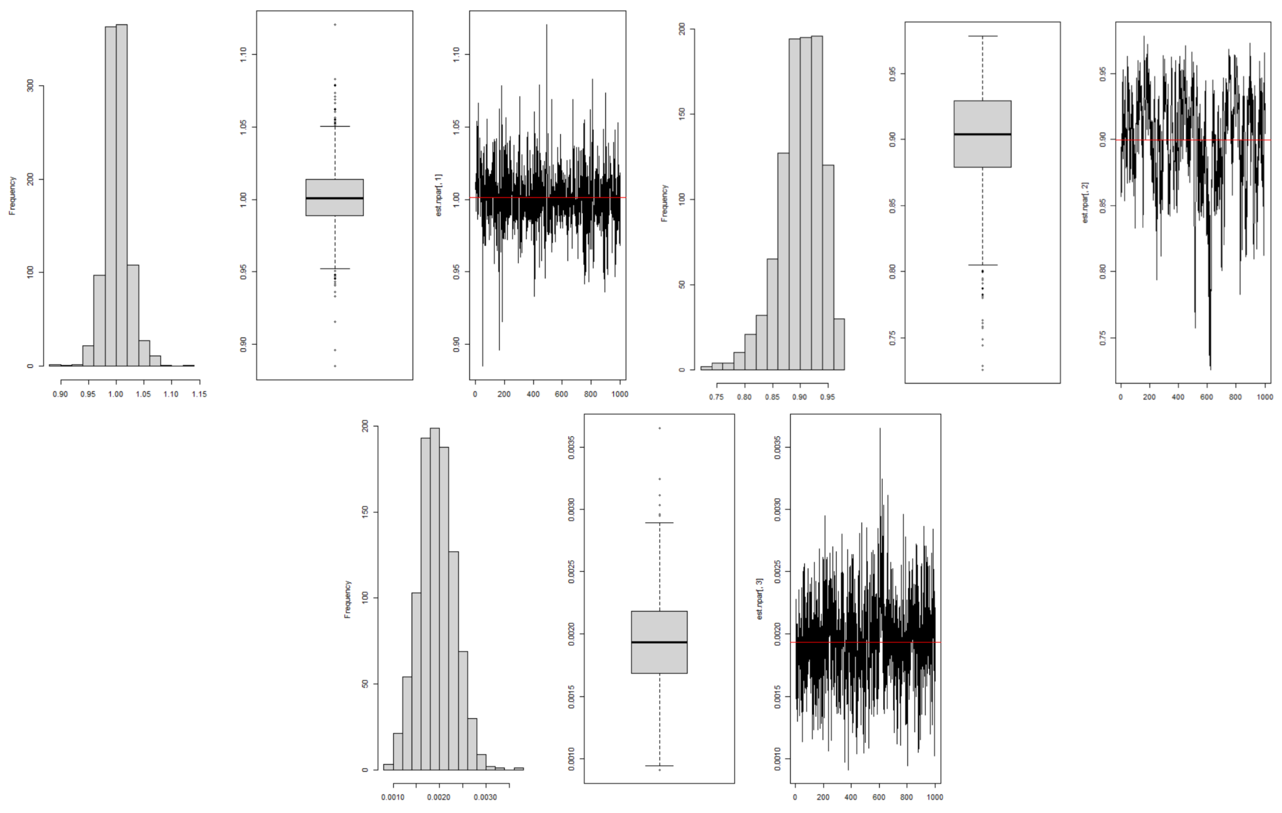
In this study, we considered B = 1000 replicates. Thus, at the end of this procedure, we have 1000 estimates, , of the vector of unknown parameters , i.e., of each of the parameters. These bootstrap estimates make it possible to obtain a bootstrap distribution to construct a bootstrap confidence interval at the level by the empirical quantiles of this distribution utilized, of order and . In this context, the bootstrap estimate of the parameter is considered to be the average of the 1000 bootstrap estimates obtained in the previous procedure.
The main advantage of this approach is that it does not require the assumption of normality or the implementation of optimization methods, as in the case of the maximum likelihood, which in some cases, may not converge or may converge to a local maximum. On the other hand, even if normality is verified, the distribution-free approach can provide initial estimates for the iterative log-likelihood optimization procedure.
2.4. Simulation Study
To analyze the performance of the proposed methodology in comparison with the maximum likelihood estimation, a simulation study was designed with various scenarios. These scenarios were based on a time-invariant state-space model defined by
where the state process
is a stationary AR(1) process with zero mean. This study was designed under the optimum conditions for maximum likelihood estimation, since errors with a normal distribution were considered, so we compared the proposed methodology in the best scenario in favor of Gaussian maximum likelihood estimation. Thus, the time series were obtained by simulating errors with the distributions
and
, considering time series of dimension
, autoregressive parameter values of 0.5 and 0.9, and two pairs of variances
.
In the scenario of large time series (
) (
Table 1 and
Table 2), which is the most-favorable scenario for maximum likelihood estimation because it enhances the convergence of the optimization method, it can be seen that distribution-free estimation associated with the bootstrap methodology had a very similar parameter estimation performance to the maximum likelihood estimation. On the one hand, the GML method performed better, particularly in terms of the confidence interval coverage rates for the highest value of the autoregressive parameter,
, but on the other hand, it had lower coverage rates at the 95% confidence level. On the other hand, DFb maintained higher coverage rates in both cases close to 100%, which means that the DFb method is conservative. In short, the proposed DFb method is more advantageous in the case of large time series when the correlation structure, translated by the
parameter, is weaker (
closer to zero). This is also evident from the analysis of the average amplitudes of the confidence intervals, which are smaller in this scenario, without a reduction in their coverage rate.
Table 3 and
Table 4 show the results of the simulation study for small time series, in this case with
, for the various combinations of the parameters
and variances. For series of this size, both estimation methods lowered their rate of valid estimates, i.e., within the parameter space. However, it can be seen that the distribution-free method associated with the bootstrapping performed best in this respect, while the Gaussian maximum likelihood estimation had the lowest success rates, especially for
. From the point of view of the accuracy of the estimates, from the RMSE perspective, the distribution-free method with the bootstrap had the best performance overall. This better performance also occurred in the analysis of the coverage rates of the confidence intervals, as well as in the analysis of their average amplitude, with this method producing confidence intervals with smaller amplitudes without compromising the coverage rate (which is still higher, as a rule, than the confidence level considered).
3. Application to Economic Data
In this section, we implement the proposed methodology on real economic data and juxtapose it with the Gaussian maximum likelihood estimation, considering both the parameter estimation and forecast quality.
3.1. Dataset
The ISM index chosen to illustrate an application to real data is the Manufacturing PMI, which is a monthly economic indicator of the United States of America. It is constructed through surveys conducted with purchasing managers in over 300 industrial companies. This index is a fundamental indicator for assessing and monitoring the development of the American economy. It was created by the “Institute for Supply Management”, from which the designation ISM derives. This non-governmental, non-profit organization organization was established in 1915 and provides reports on development, education, and research to both individuals and companies or financial institutions with the purpose of creating value and enabling them to gain competitive advantages, as this information supports many decision-making processes in management.
The Manufacturing PMI index allows the analysis of changes in production levels between months. The reports are released on the first business day of a given month, making it one of the first economic indicators available to managers and investors. It is composed of five other subindicators with equal weight, as described by [
25]. These subindicators are:
New Orders, reflecting the number of customer orders placed with companies;
Production, evaluating whether a company’s production has changed compared to a previous period (days, weeks, and months);
Employment, measuring changes in employment, whether it has increased or decreased;
Deliveries, revealing whether the delivery times between suppliers and the company have increased or decreased compared to a previous period;
Inventories, indicating how much a company’s inventories have increased or decreased.
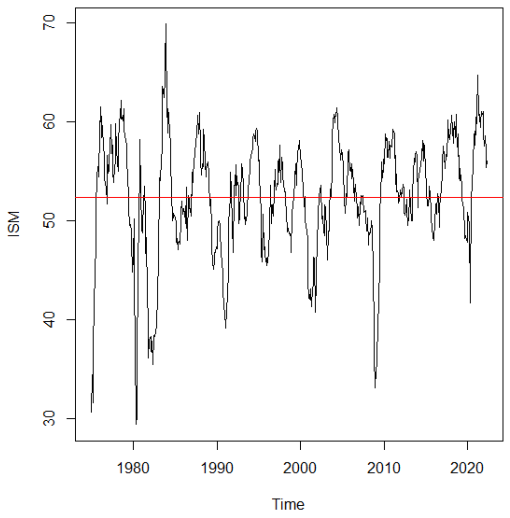
The companies were categorized into 18 different sectors, including food and beverages, chemicals, machinery, and transportation equipment, among others. In summary, the data from the ISM Manufacturing Index, especially the PMI, allows for a comprehensive assessment of the performance of the U.S. manufacturing industry. The database, named “ISM”, considered in this work comprises 569 observations, including monthly ISM values and their respective dates. The time series analyzed included values from January 1975 up to May 2022. The data are reported on a monthly basis. For the purposes of modeling and estimating the models, a training time series up to December 2020 was considered (
Figure 1), leaving the last observations for the model testing and evaluation series.
Figure 1 shows that the series may not be stationary in terms of variance. There were several oscillations throughout the series, most notably in the 1980s, between 2007 and 2010, as well as between 2019 and 2022. The minimum value of 29.40 in April 1980 reflects a period in which the economy was already in recession; in that decade, the unemployment rate was around 7.5%. Both the 1980 recession and the 1981–82 recessions were triggered by a restrictive monetary policy in an attempt to combat rising inflation. During the 1960s and 1970s, economists and policymakers believed that they could reduce unemployment through higher inflation, in a trade-off known as the Philips curve. This strategy severely affected U.S. industrial companies [
26]. The maximum observed value of 69.90 was obtained after the recovery from the aforementioned recession.
3.2. Modeling with Regression Linear Models
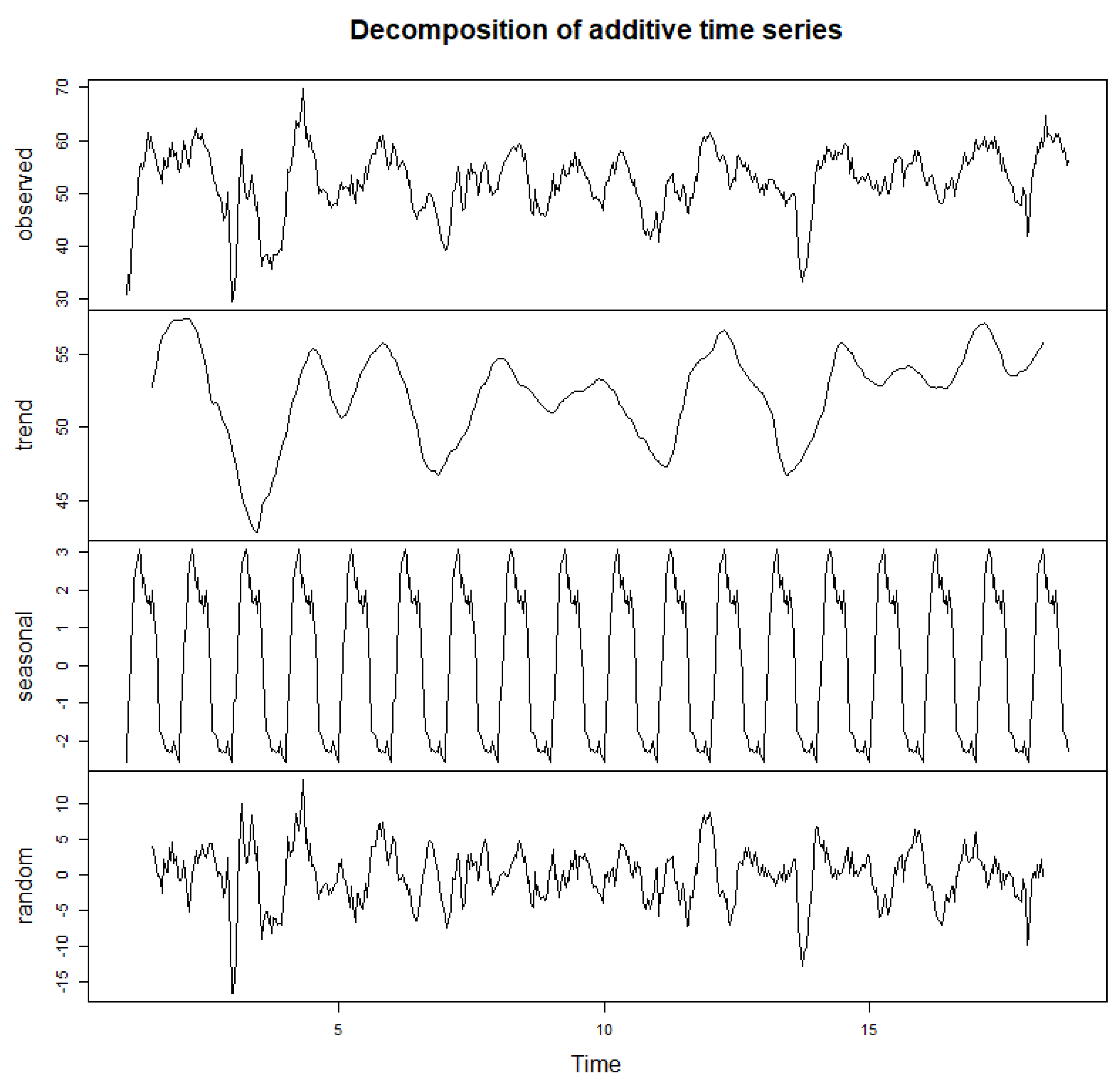
To identify possible components in the ISM index time series, it was broken down into the usual level, trend, seasonality, and noise components (
Figure 2). The breakdown of the time series indicated a possible trend and a seasonal component, with a 12-month period, if any, and low amplitude (of around −2 to 3 points). Based on this exploratory analysis of the time series, a linear model and a state-space model will be adjusted and analyzed, whose performance will be evaluated.
By examining
Figure 2, it can be observed that the seasonal component was extremely small. To assess the significance of the seasonal component and trend, a model was fit with a set of explanatory variables, including indicators for 11 months, the intercept term, the independent variable time (since we already confirmed the presence of a trend), and the response variable, the ISM series. The indicator variables were also considered dummy variables. The multiple linear regression model included the intercept term
, the coefficient
associated with the time variable
, dummy variables
, where
, representing indicator variables
, which assumes 1 when month
t is January (
), …, November (
), and the random error
, that is
Table 5 represents the estimates and their corresponding
p-values for the estimated parameters of the multiple linear regression model. At a significance level of
, only the intercept,
, and the coefficient associated with the time variable,
, had
p-values below
, which means that the seasonal coefficients were not statistically significant when considering the annual seasonality. Thus, the linear trend component will be the only one considered in the linear modeling.
In
Table 6 is presented the summary of the simple linear regression model with the time variable, since the coefficients associated with the seasonal variables were not statistically significant.
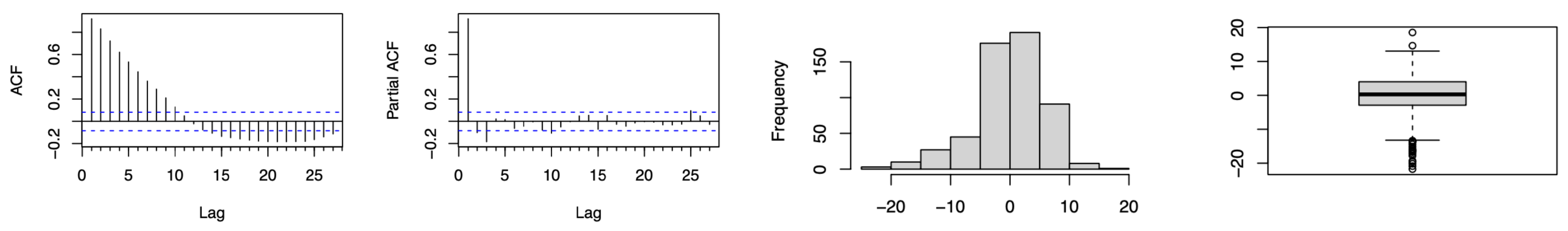
The histogram in
Figure 3 shows that the residuals did not behave like a white noise process. The Shapiro–Wilk and the Kolmogorov–Smirnov normality tests rejected the null hypothesis that the residuals were normal. The analysis of the autocorrelation function (ACF) and the partial autocorrelation function (PACF) graphs showed that the residuals also had a temporal correlation structure.
3.3. SARIMA Modeling
In order to have a model that can incorporate a temporal correlation structure, several SARIMA models were fit to the ISM index time series. From this analysis, the best-performing model was
, with the following formulation:
and whose summary is shown in
Table 7.
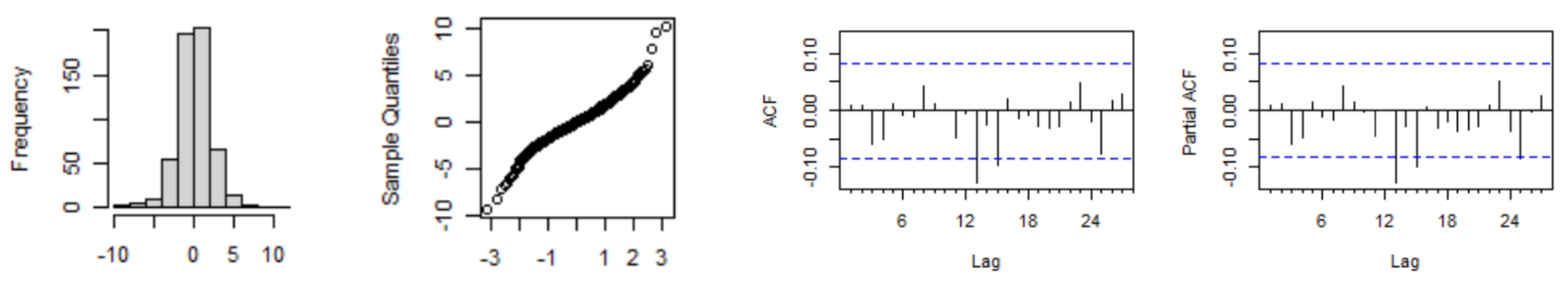
The analysis of the SARIMA model’s residuals showed that the normality of their distribution was rejected (
Figure 4). However, the Ljung–Box test did not reject the hypothesis that there was no correlation in the series of residuals, considering lags up to 24.
3.4. State-Space Modeling
In order to be able to integrate the temporal correlation structure already identified, either by adjusting the simple linear regression model or by the SARIMA model, we also considered a state-space model in which the known values
were the predicted values resulting from adjusting the simple linear regression model. In this way, we considered a state-space model with the following observation equation:
where
, with
and the state process
is an autoregressive process:
This state-space model can be understood as a calibration model in which the linear trend with the base structure is considered, which is calibrated, at each moment t, by a stochastic factor . This model makes it possible to incorporate a temporal correction structure, in this case through the state process, and a dynamic adjustment over time. We would expect the average of the calibration factor process to be close to 1, with each calibration factor corresponding to a correction factor that either increases the value expected by the trend, , or decreases it, .
This model was adjusted and its unknown parameters,
, estimated by both the maximum likelihood method with the assumption of normality of the errors
and
and the distribution-free estimators proposed in [
13]. The standard errors and confidence intervals of the latter were obtained via bootstrapping. The results of the parameter estimation and the respective confidence intervals at
are shown in
Table 8. In both estimation methods, the estimation of the observation error variance was zero. This implies that, in practice, the response variable—in this case, the ISM index—is explained by the calibration of the linear trend,
, through the autoregressive order -one state process without additional noise. However, it should be noted that the resulting model is heteroscedastic, as the variance of the response variable,
, is given by
, given that the state process,
, is stationary (
< 1). From the analysis of the results, it can be concluded that both estimation methods provide very similar point estimates of the parameters. However, the most-significant difference lies in
, with the maximum likelihood estimation estimating this variance at about 15-times the value of the non-parametric estimate.
With regard to the maximum likelihood estimation, the standardized innovations must be analyzed to see if they behave like white noise. From the analysis of the standardized innovations,
Table 9, and the tests for normality and correlation, we rejected the normality and the hypothesis of no correlation, indicating that the assumptions of the model and normality do not hold.
The standard errors and bootstrap confidence intervals were obtained from the empirical bootstrap distributions obtained from the 1000 replicates obtained for each parameter; see
Figure 5. The descriptive statistics of the bootstrap distributions are shown in
Table 10. The maximum likelihood estimation, although dependent on the assumptions about the distribution of errors, still provided interesting results from a modeling perspective, and the differences compared to non-parametric estimation were not significant. This suggests that, despite the challenges observed in the assumptions of the maximum likelihood estimation, this method remains a robust tool for the analysis of state-space models, at least in the specific application of this study. On the other hand, the non-parametric approach allowed overcoming the limitations associated with the normality assumption.
3.5. Forecasting
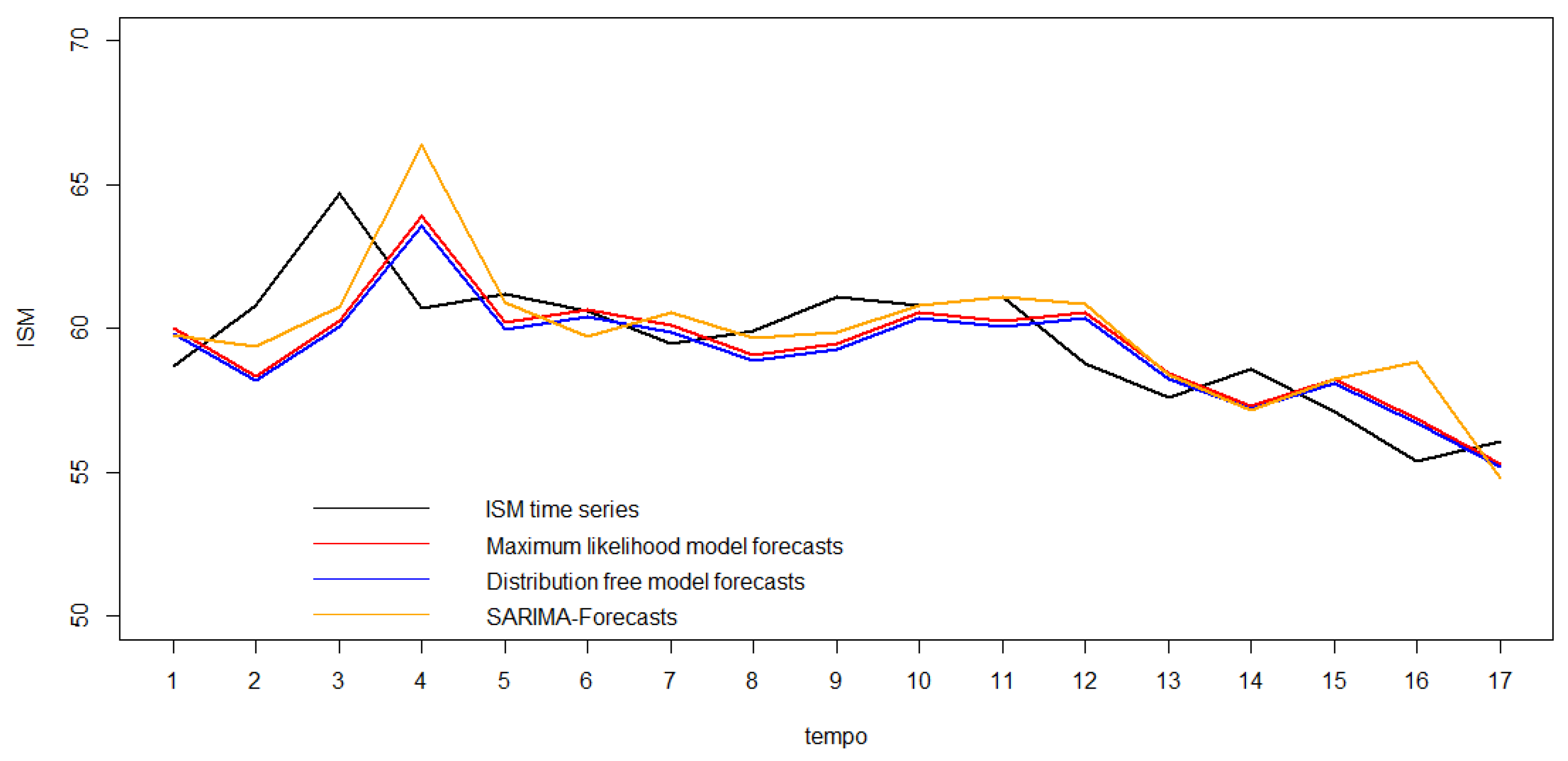
In this section, we present the forecasting procedure in a statistical modeling context, focusing on the three fitted models. The period for which one-step-ahead forecasts are desired corresponds to the test series, that is it extends from January 2021 to May 2022, comprising a total of 17 observations. Forecasts will be obtained through three different models: the simple linear regression model (SLRM), the SARIMA model (SARIMA), and the state-space model, whose parameters were estimated using both the Gaussian maximum likelihood (SSM-GML) and the distribution-free estimators associated with the use of bootstrapping to estimate the standard errors and confidence intervals (SSM-DFb).
Table 11, complemented by the analysis of the graphs in
Figure 6, allows us to conclude that the state-space models performed best in terms of the accuracy of the one-step predictions in the test series. These values were used to fit the two state-space models. The lowest MSE was obtained when considering the state-space model with the Gaussian maximum likelihood parameter estimation; however, the SSM-DFb model had a very similar RMSE, with no significant statistical difference (the
p-value of the Diebold–Mariano test was 0.3981 [
27]). The SARIMA model forecasts, on the other hand, had a higher root-mean-squared error.
When we analyzed the confidence intervals of the 17 one-step-ahead forecasts based on the maximum likelihood estimation and distribution-free bootstrap estimators, it can be seen that the latter produced bootstrap confidence intervals with an average semi-range of , while the Gaussian maximum likelihood estimation produced a value of . In addition, in both methods, only one of the observations did not match the respective prediction intervals, corresponding to 5.9%, a value close to the significance level considered. In this particular case, the SARIMA model produced confidence intervals with average semi-amplitudes of 4.17, i.e., slightly lower than with the other models, and as already mentioned, from the point of view of point forecasting, it performed worse in terms of the root-mean-squared error of the point forecasts for these 17 forecast instants.


 ,
, 


