
Improvement on Forecasting of Propagation of the COVID-19 Pandemic through Combining Oscillations in ARIMA Models


Abstract
:1. Introduction
2. Method
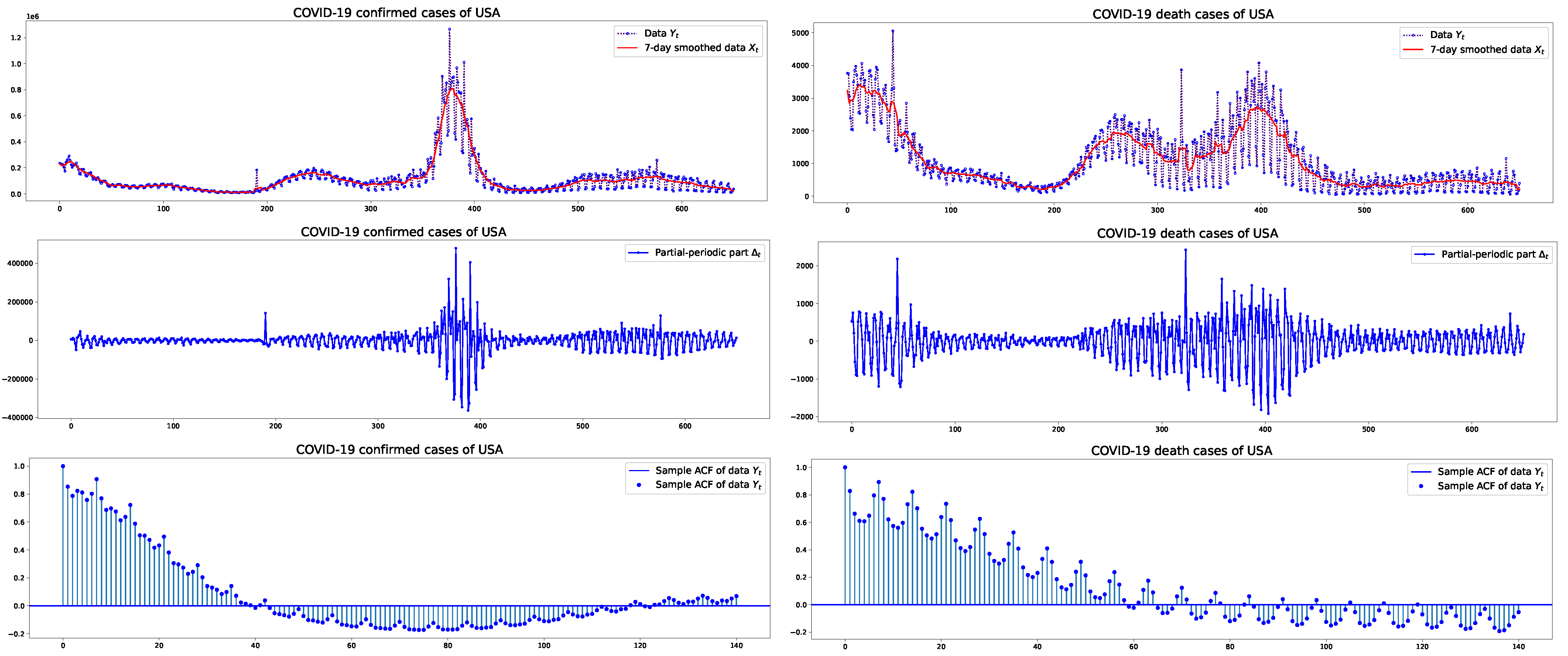
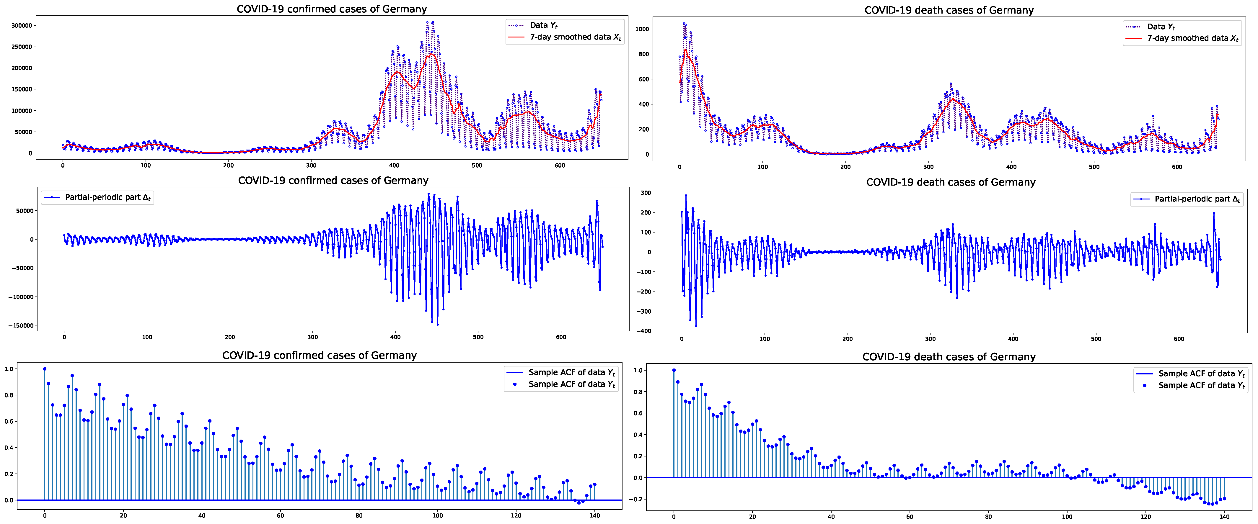
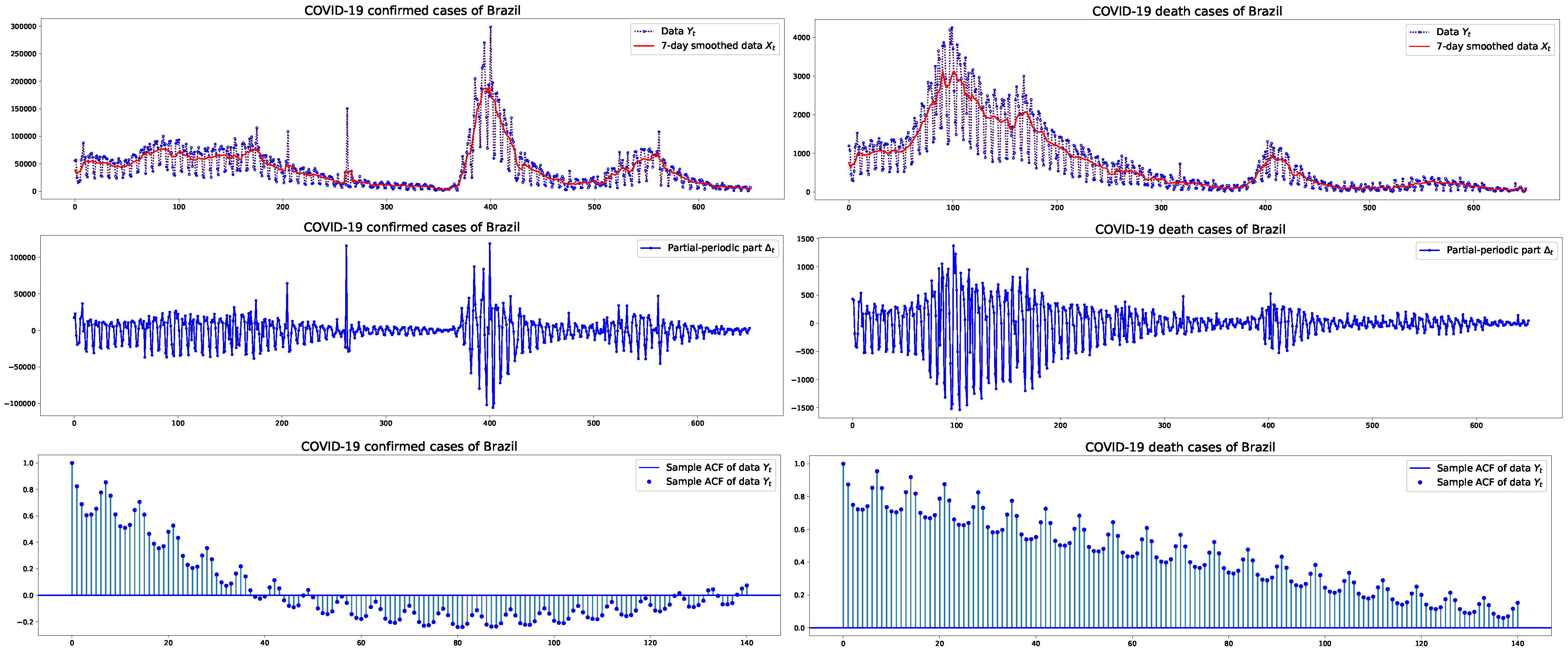
2.1. Data
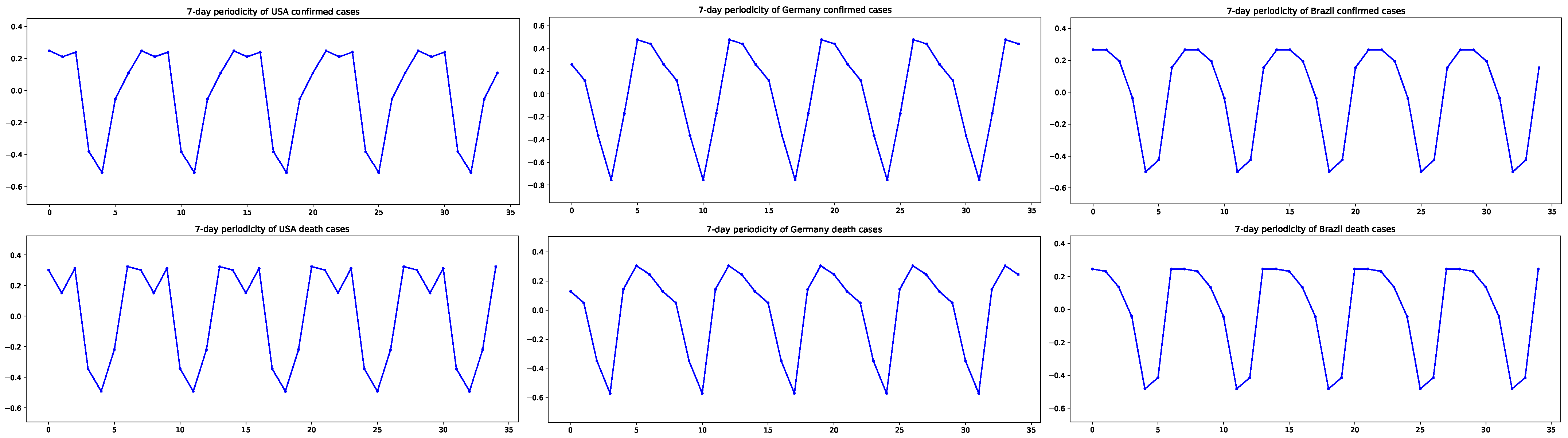
2.2. ARIMA Model with Partial Periodic Oscillation
2.3. Estimation
3. Results
3.1. Estimation Results
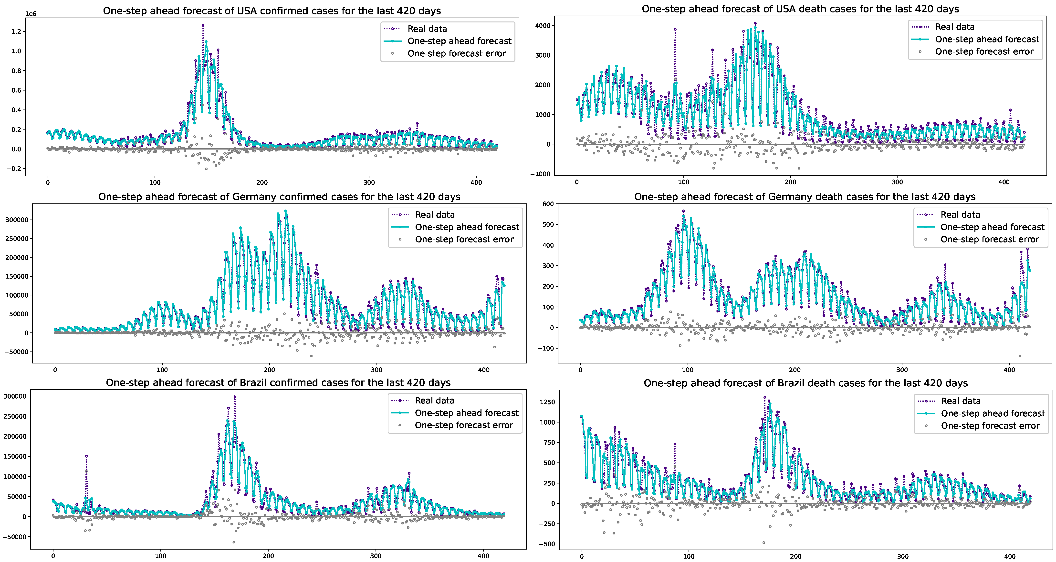
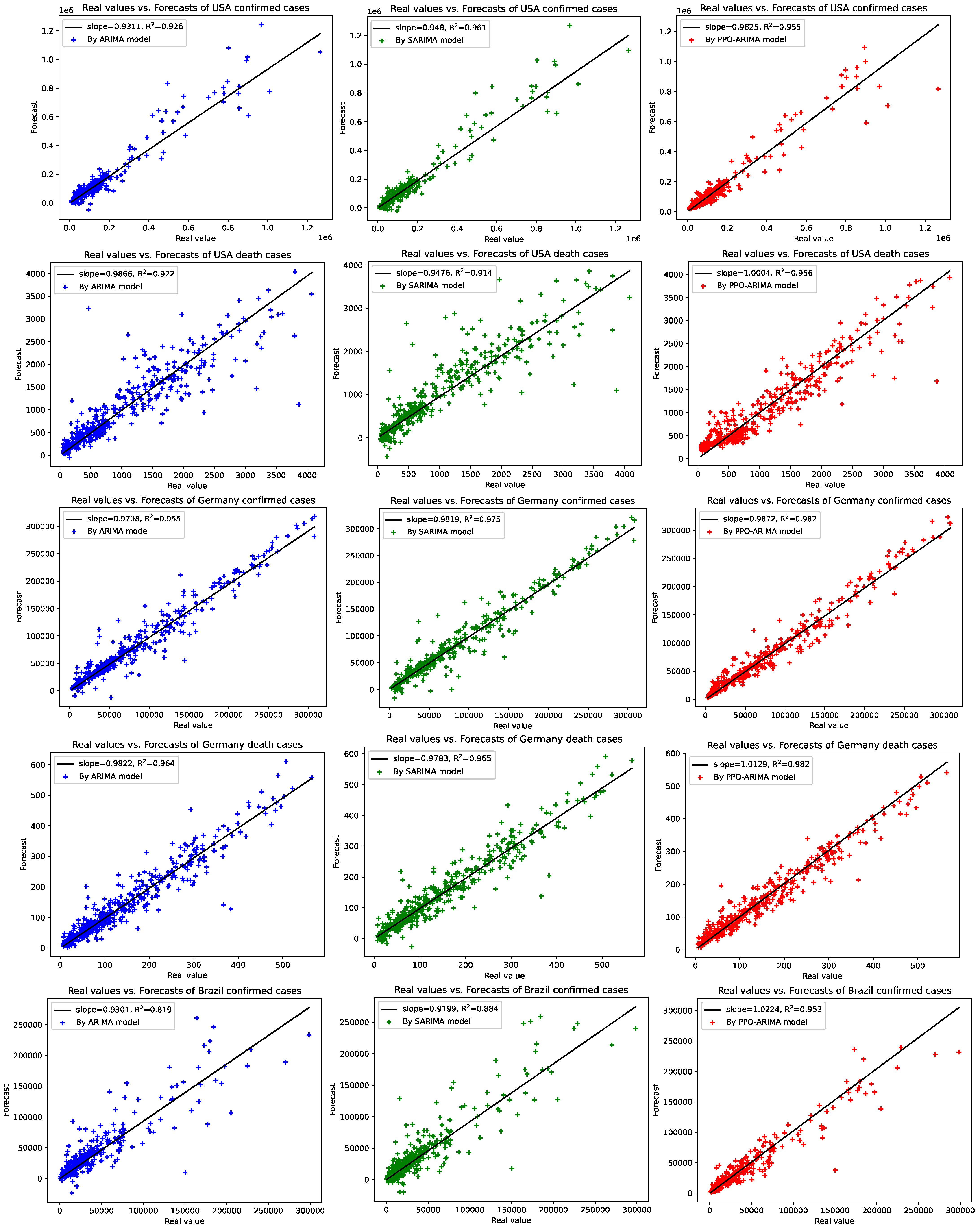
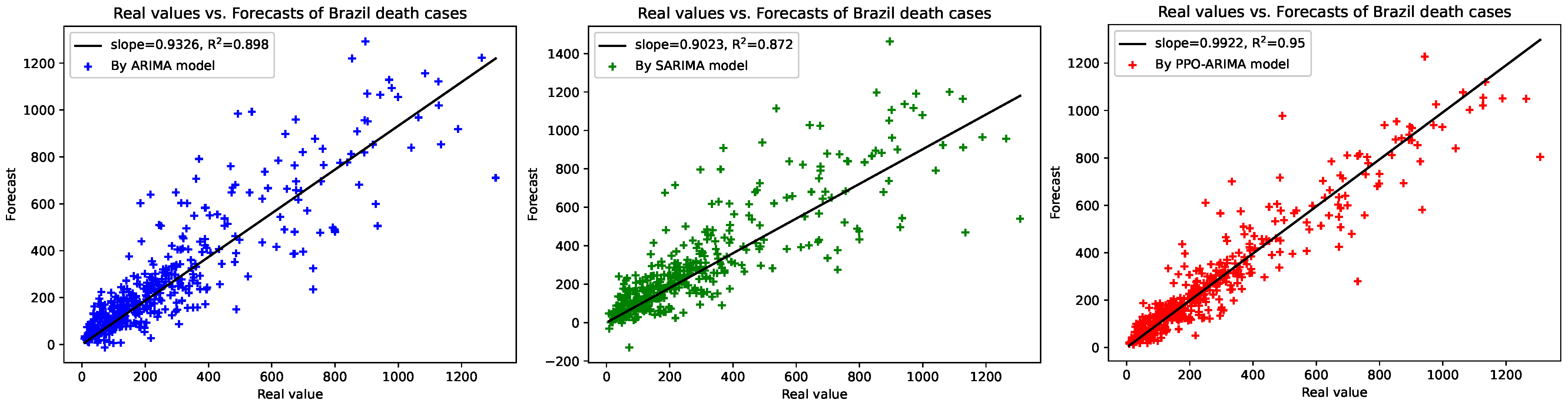
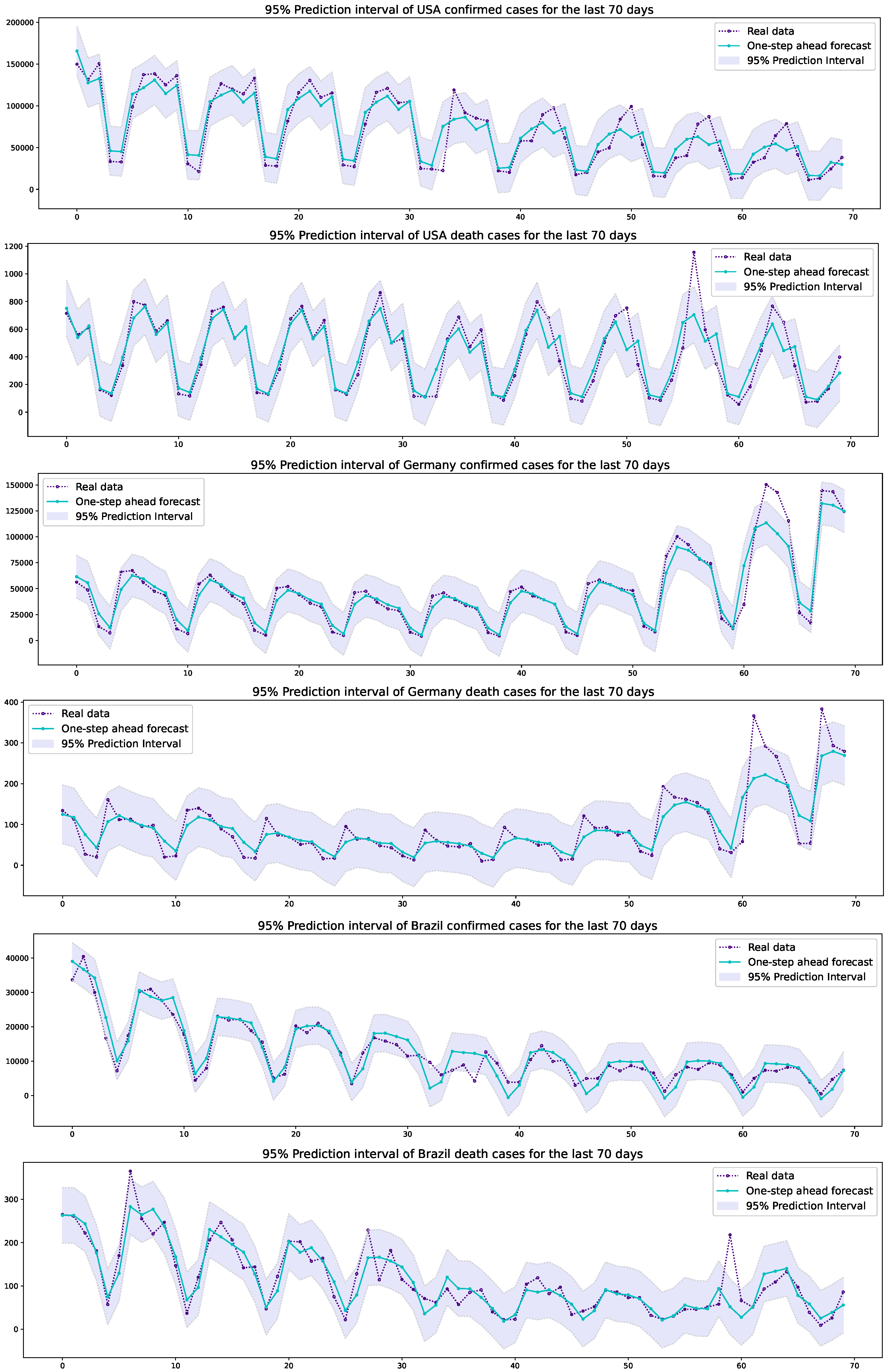
3.2. Prediction Results
4. Discussion and Conclusions
Funding
Data Availability Statement
Acknowledgments
Conflicts of Interest
References
- Ribeiro, M.H.D.M.; Silva, R.G.D.; Mariani, V.C.; Coelho, L.D.S. Short-term forecasting COVID-19 cumulative confirmed cases: Perspectives for Brazil. Chaos Solitons Fractals 2020, 135, 109853. [Google Scholar] [CrossRef] [PubMed]
- Maleki, M.; Mahmoudi, M.; Wraith, D.; Pho, K. Time series modelling to fore cast the confirmed and recovered cases of COVID-19. Travel. Med. Infect. Dis. 2020, 37, 101742. [Google Scholar] [CrossRef] [PubMed]
- Maleki, M.; Mahmoudi, M.R.; Heydari, M.H. Modeling and forecasting the spread and death rate of coronavirus (COVID-19) in the world using time series models. Chaos Solitons Fractals 2020, 140, 110151. [Google Scholar] [CrossRef] [PubMed]
- Sarkar, K.; Khajanchi, S.; Nieto, J.J. Modeling and forecasting the COVID-19 pandemic in India. Chaos Solitons Fractals 2020, 139, 110049. [Google Scholar] [CrossRef] [PubMed]
- Balli, S. Data analysis of COVID-19 pandemic and short-term cumulative case forecasting using machine learning time series methods. Chaos Solitons Fractals 2021, 142, 110512. [Google Scholar] [CrossRef] [PubMed]
- Ala’raj, M.; Majdalawieh, M.; Nizamuddin, N. Modeling and forecasting of COVID-19 using a hybrid dynamic model based on SEIRD with ARIMA corrections. Infect. Dis. Model. 2021, 6, 98–111. [Google Scholar] [CrossRef]
- Kumar, Y.; Koul, A.; Kaur, S.; Hu, Y.C. Machine learning and deep learning based time series prediction and forecasting of ten nations’ COVID-19 pandemic. SN Comput. Sci. 2022, 4, 91. [Google Scholar] [CrossRef] [PubMed]
- Fang, L.; Wang, D.; Pan, G. Analysis and estimation of COVID-19 spreading in Russia based on ARIMA model. Sn Compr. Clin. Med. 2020, 2, 2521–2527. [Google Scholar] [CrossRef]
- Ilie, O.D.; Cojocariu, R.O.; Ciobica, A.; Timofte, S.I.; Mavroudis, I.; Doroftei, B. Fore casting the spreading of COVID-19 across Nine countries from Europe, Asia, and the American continents using the ARIMA Models. Microorganisms 2020, 8, 1158. [Google Scholar] [CrossRef]
- Toğa, G.; Atalay, B.; Toksari, M.D. COVID-19 prevalence forecasting using Autoregressive Integrated Moving Average (ARIMA) and Artifcial Neural Networks (ANN): Case of Turkey. J. Infect. Public Health 2021, 14, 811–816. [Google Scholar] [CrossRef]
- Bartolomeo, N.; Trerotoli, P.; Serio, G. Short-term forecast in the early stage of the COVID-19 outbreak in Italy. Application of a weighted and cumulative average daily growth rate to an exponential decay model. Infect. Dis. Model. 2021, 6, 212–221. [Google Scholar] [CrossRef] [PubMed]
- Petropoulos, F.; Makridakis, S.; Stylianou, N. COVID-19: Forecasting confirmed cases and deaths with a simple time series model. Int. J. Forecast. 2022, 38, 439–452. [Google Scholar] [CrossRef] [PubMed]
- Lourenco, J.; Recker, M. Natural, persistent oscillations in a spartial multi-strain disease system with application to dengue. PLoS Comput. Biol. 2013, 9, e1003308. [Google Scholar] [CrossRef] [PubMed]
- Selvaraj, P.; Wenger, E.A.; Gerardin, J. Seasonality and heterogeneity of malaria transmission determine success of interventions in high-endemic settings: A modeling study. BMC Infect. Dis. 2018, 18, 413. [Google Scholar] [CrossRef] [PubMed]
- Polwiang, S. The time series seasonal patterns of dengue fever and associated weather variables in Bangkok (2003–2017). BMC Infect. Dis. 2020, 20, 208. [Google Scholar] [CrossRef] [PubMed]
- Yuan, H.; Kramer, S.C.; Lau, E.H.Y.; Cowling, B.J.; Yang, W. Modeling influenza seasonality in the tropics and subtropics. PLoS Comput. Biol. 2021, 17, e1009050. [Google Scholar] [CrossRef] [PubMed]
- Li, Z.; Zhang, T. Analysis of a COVID-19 epidemic model with seasonality. Bull. Math. Biol. 2022, 84, 146. [Google Scholar] [CrossRef]
- Ndlovu, M.; Moyo, R.; Mpofu, M. Modelling COVID-19 infection with seasonality in Zimbabwe. Phys. Chem. Earth Parts A/B/C 2022, 127, 103167. [Google Scholar] [CrossRef]
- Wiemken, T.L.; Khan, F.; Puzniak, L.; Yang, W.; Simmering, J.; Polgreen, P.; Nguyen, J.L.; Jodar, L.; McLaughlin, J.M. Seasonal trends in COVID-19 cases, hospitalizations, and mortality in the United States and Europe. Sci. Rep. 2023, 13, 3886. [Google Scholar] [CrossRef]
- Bukhari, Q.; Jameel, Y.; Massaro, J.M.; D’Agostino, R.B.; Khan, S. Periodic oscillations in daily reported infections and deaths for coronavirus disease 2019. JAMA Netw. Open 2020, 3, e2017521. [Google Scholar] [CrossRef]
- Bergman, A.; Sella, Y.; Agre, P.; Casadevall, A. Oscillations in U.S. COVID-19 incidence and mortality data reflect diagnostic and reporting factors. mSystems 2020, 5, e00544-20. [Google Scholar] [CrossRef] [PubMed]
- Dehning, J.; Zierenberg, J.; Spitzner, F.P.; Wibral, M.; Neto, J.P.; Wilczek, M.; Priesmann, V. Inferring change points in the spread of COVID-19 reveals the effectiveness of interventions. Science 2020, 369, 160. [Google Scholar] [CrossRef] [PubMed]
- Huang, J.; Liu, X.; Zhang, L.; Zhao, Y.; Wang, D.; Gao, J.; Lian, X.; Liu, C. The oscillation-outbreak characteristic of the COVID-19 pandemic. Natl. Sci. Rev. 2021, 8, nwab100. [Google Scholar] [CrossRef] [PubMed]
- Soukhovolsky, V.; Kovalev, A.; Pitt, A.; Shulman, K.; Tarasova, O.; Kessel, B. The cyclicity of coronavirus cases: “Waves” and the “weekend effect”. Chaos Solitons Fractals 2021, 114, 110718. [Google Scholar] [CrossRef] [PubMed]
- Campi, G.; Bianconi, A. Periodic recurrent waves of Covid-19 epidemics and vaccination campaign. Chaos Solitons Fractals 2022, 160, 112216. [Google Scholar] [CrossRef] [PubMed]
- Simeonov, O.; Eaton, C.D. Modeling the drivers of oscillations in COVID-19 data on college campuses. Ann. Epidemiol. 2023, 82, 40–44. [Google Scholar] [CrossRef] [PubMed]
- Ekinci, A. Modeling and forecasting of growth rate of new COVID-19 cases in top nine affected countries: Considering conditional variance and asymmetric effect. Chaos Solitons Fractals 2021, 151, 111227. [Google Scholar] [CrossRef] [PubMed]
- Hwang, E. Prediction intervals of the COVID-19 cases by HAR models with growth rates and vaccination rates in top eight affected countries: Bootstrap improvement. Chaos Solitons Fractals 2022, 155, 111789. [Google Scholar] [CrossRef]
- Ceylan, Z. Estimation of COVID-19 prevalence in Italy, Spain and France. Sci. Total Environ. 2020, 729, 138817. [Google Scholar] [CrossRef]
- Selinger, C.; Choist, M.; Alison, S. Predicting COVID-19 incidence in French hospitals using human contact network analytics. Int. J. Infect. Dis. 2021, 111, 100–107. [Google Scholar] [CrossRef]


| USA | Germany | Brazil | ||||
|---|---|---|---|---|---|---|
| C | D | C | D | C | D | |
| Mean | 116,581.67 | 1079.81 | 50,280.45 | 161.85 | 41,745.69 | 759.27 |
| SD | 148,459.10 | 969.73 | 64,236.28 | 165.32 | 39,735.55 | 862.98 |
| Min | 8275 | 49 | 208 | 0 | 0 | 0 |
| Median | 76,415.0 | 703.0 | 20,841.0 | 113.0 | 30,671.0 | 361.0 |
| Max | 1,265,520 | 5061 | 307,935 | 1045 | 298,408 | 4249 |
| Skewness | 3.85 | 1.3 | 1.83 | 2.13 | 2.16 | 1.63 |
| Kurtosis | 17.74 | 1.01 | 2.88 | 6.33 | 7.03 | 2.25 |
| USA | Germany | Brazil | ||||
|---|---|---|---|---|---|---|
| C | D | C | D | C | D | |
| Test statistics | −2.7255 | −3.9143 | −1.6715 | −2.5841 | −3.967 | −1.8058 |
| p-value | 0.0697 | 0.0019 | 0.4458 | 0.0963 | 0.0016 | 0.3776 |
| orders ( | (1,1,2) | (1,0,1) | (1.1.1) | (1,1,2) | (1,0,2) | (1,1,2) |
| 0.9562 | 0.9986 | 0.4115 | 0.9621 | 0.9913 | 0.9499 | |
| (0.005) | (0.004) | (0.028) | (0.005) | (0.003) | (0.017) | |
| −0.7722 | 0.2703 | 0.4279 | −0.4833 | 0.1981 | −0.6314 | |
| (0.014) | (0.025) | (0.025) | (0.016) | (0.019) | (0.029) | |
| 0.2012 | - | - | −0.1788 | 0.2308 | −0.1951 | |
| (0.021) | - | - | (0.016) | (0.027) | (0.022) | |
| USA | Germany | Brazil | ||||
|---|---|---|---|---|---|---|
| C | D | C | D | C | D | |
| −0.7295 | −1.063 | −0.7795 | −0.9788 | −1.0506 | −0.8798 | |
| 1.02 | 1.358 | 1.13 | 0.956 | 0.90 | 0.794 | |
| 0.2486 | 0.3020 | 0.2609 | 0.1287 | 0.2661 | 0.2453 | |
| 0.2113 | 0.1514 | 0.1188 | 0.0492 | 0.2660 | 0.2314 | |
| 0.2399 | 0.3126 | −0.3643 | −0.3501 | 0.1948 | 0.1355 | |
| −0.3816 | −0.3443 | −0.7460 | −0.5727 | −0.0373 | −0.0437 | |
| −0.5119 | −0.4915 | −0.1698 | 0.1421 | −0.4992 | −0.4823 | |
| −0.0525 | −0.2193 | 0.4784 | 0.3045 | −0.4243 | −0.4141 | |
| 0.1104 | 0.3235 | 0.4415 | 0.2448 | 0.1542 | 0.2450 | |
| USA | Germany | Brazil | ||||||
|---|---|---|---|---|---|---|---|---|
| -Step | C | D | C | D | C | D | ||
| RMSE | ARIMA | 1 | 0.3335 | 0.3901 | 0.2457 | 0.2185 | 0.4915 | 0.1436 |
| 2 | 0.6597 | 0.6155 | 0.6118 | 0.4143 | 0.6432 | 0.2039 | ||
| 3 | 0.7821 | 0.8225 | 0.9098 | 0.5764 | 0.8162 | 0.2624 | ||
| SARIMA | 1 | 0.3086 | 0.4115 | 0.2520 | 0.2155 | 0.4985 | 0.1635 | |
| 2 | 0.6947 | 0.7014 | 0.6262 | 0.4331 | 0.6388 | 0.2259 | ||
| 3 | 0.8171 | 0.9384 | 0.9251 | 0.5977 | 0.8281 | 0.2832 | ||
| PPO-ARIMA | 1 | 0.3153 | 0.2920 | 0.2027 | 0.1669 | 0.3152 | 0.0989 | |
| 2 | 0.4901 | 0.5348 | 0.4648 | 0.3419 | 0.5001 | 0.1865 | ||
| 3 | 0.5306 | 0.7867 | 0.8325 | 0.5358 | 0.5857 | 0.1926 | ||
| MAE | ARIMA | 1 | 0.1729 | 0.2307 | 0.1446 | 0.1413 | 0.2609 | 0.0940 |
| 2 | 0.3397 | 0.4184 | 0.4093 | 0.2919 | 0.3772 | 0.1376 | ||
| 3 | 0.4578 | 0.6014 | 0.6365 | 0.4340 | 0.4888 | 0.1834 | ||
| SARIMA | 1 | 0.1571 | 0.2361 | 0.1459 | 0.1441 | 0.2813 | 0.1031 | |
| 2 | 0.3521 | 0.4722 | 0.4164 | 0.3048 | 0.3837 | 0.1527 | ||
| 3 | 0.4817 | 0.6895 | 0.6485 | 0.4453 | 0.5107 | 0.1976 | ||
| PPO-ARIMA | 1 | 0.1615 | 0.1994 | 0.1287 | 0.1077 | 0.1650 | 0.0614 | |
| 2 | 0.2672 | 0.3691 | 0.3008 | 0.2339 | 0.2670 | 0.1119 | ||
| 3 | 0.3133 | 0.5509 | 0.5599 | 0.3931 | 0.3207 | 0.1355 | ||
| HMAE | ARIMA | 1 | 0.2327 | 0.3421 | 0.2038 | 0.2526 | 0.4161 | 0.4318 |
| 2 | 0.5237 | 0.7645 | 0.5549 | 0.4798 | 0.6921 | 0.7285 | ||
| 3 | 0.8004 | 1.2584 | 0.9726 | 0.7974 | 0.9736 | 0.9928 | ||
| SARIMA | 1 | 0.2081 | 0.3805 | 0.2063 | 0.2817 | 0.5245 | 0.4542 | |
| 2 | 0.5375 | 0.9115 | 0.5753 | 0.5315 | 0.7613 | 0.8382 | ||
| 3 | 0.8292 | 1.5192 | 1.0082 | 0.8297 | 1.0043 | 1.0679 | ||
| PPO-ARIMA | 1 | 0.2330 | 0.3998 | 0.2008 | 0.2157 | 0.3463 | 0.2946 | |
| 2 | 0.4450 | 0.7436 | 0.6071 | 0.5271 | 0.4756 | 0.5286 | ||
| 3 | 0.5961 | 1.2010 | 1.1289 | 0.9019 | 0.6949 | 0.8046 | ||
| USA | Germany | Brazil | ||||||
|---|---|---|---|---|---|---|---|---|
| -Step | C | D | C | D | C | D | ||
| RMSE | Effi | 1 | 5.80 | 33.59 | 21.21 | 30.92 | 55.93 | 45.19 |
| 2 | 34.61 | 15.09 | 31.63 | 21.18 | 28.61 | 9.33 | ||
| 3 | 47.40 | 4.55 | 9.29 | 7.57 | 39.35 | 36.24 | ||
| Effi | 1 | −2.12 | 40.92 | 24.32 | 29.12 | 58.15 | 65.32 | |
| 2 | 41.75 | 32.15 | 34.72 | 26.67 | 27.72 | 21.17 | ||
| 3 | 53.99 | 19.18 | 42.65 | 11.55 | 41.37 | 47.04 | ||
| MAE | Effi | 1 | 7.06 | 15.69 | 12.35 | 31.20 | 58.12 | 53.09 |
| 2 | 27.13 | 13.36 | 36.07 | 23.79 | 41.27 | 22.96 | ||
| 3 | 46.12 | 9.17 | 13.68 | 10.40 | 52.41 | 35.35 | ||
| Effi | 1 | −2.72 | 18.41 | 13.36 | 33.79 | 70.48 | 67.92 | |
| 2 | 31.77 | 27.93 | 38.43 | 30.31 | 43.71 | 36.46 | ||
| 3 | 53.75 | 25.16 | 15.82 | 13.28 | 59.25 | 45.83 | ||
| HMAE | Effi | 1 | −0.13 | −14.32 | 1.49 | 17.11 | 20.16 | 46.57 |
| 2 | 17.68 | 2.81 | −8.59 | −8.97 | 45.52 | 37.82 | ||
| 3 | 34.27 | 4.78 | −13.84 | −11.59 | 40.11 | 23.39 | ||
| Effi | 1 | −10.68 | −4.82 | 2.73 | 30.59 | 51.45 | 54.18 | |
| 2 | 20.78 | 22.58 | −5.23 | 0.84 | 60.09 | 58.56 | ||
| 3 | 30.10 | 26.49 | −10.69 | −8.01 | 44.52 | 32.72 | ||
Disclaimer/Publisher’s Note: The statements, opinions and data contained in all publications are solely those of the individual author(s) and contributor(s) and not of MDPI and/or the editor(s). MDPI and/or the editor(s) disclaim responsibility for any injury to people or property resulting from any ideas, methods, instructions or products referred to in the content. |
© 2023 by the author. Licensee MDPI, Basel, Switzerland. This article is an open access article distributed under the terms and conditions of the Creative Commons Attribution (CC BY) license (https://creativecommons.org/licenses/by/4.0/).
Share and Cite
Hwang, E. Improvement on Forecasting of Propagation of the COVID-19 Pandemic through Combining Oscillations in ARIMA Models. Forecasting 2024, 6, 18-35. https://doi.org/10.3390/forecast6010002
Hwang E. Improvement on Forecasting of Propagation of the COVID-19 Pandemic through Combining Oscillations in ARIMA Models. Forecasting. 2024; 6(1):18-35. https://doi.org/10.3390/forecast6010002
Chicago/Turabian StyleHwang, Eunju. 2024. "Improvement on Forecasting of Propagation of the COVID-19 Pandemic through Combining Oscillations in ARIMA Models" Forecasting 6, no. 1: 18-35. https://doi.org/10.3390/forecast6010002