
Advancements in Downscaling Global Climate Model Temperature Data in Southeast Asia: A Machine Learning Approach


Abstract
:1. Introduction
2. Materials and Methods
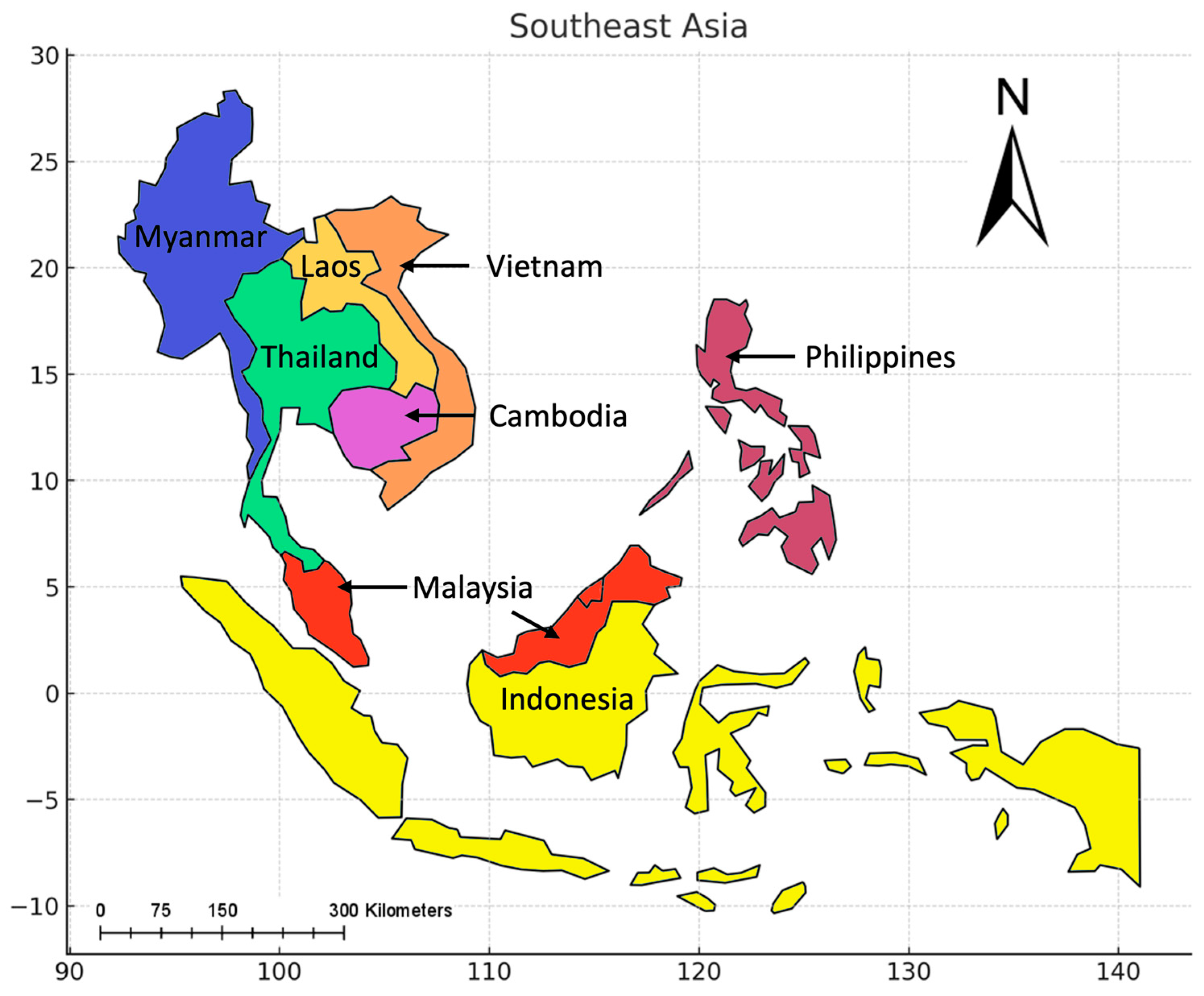
2.1. Study Area
2.2. Data Used
2.3. Statistical Used
2.4. Machine Learning (ML)
3. Results
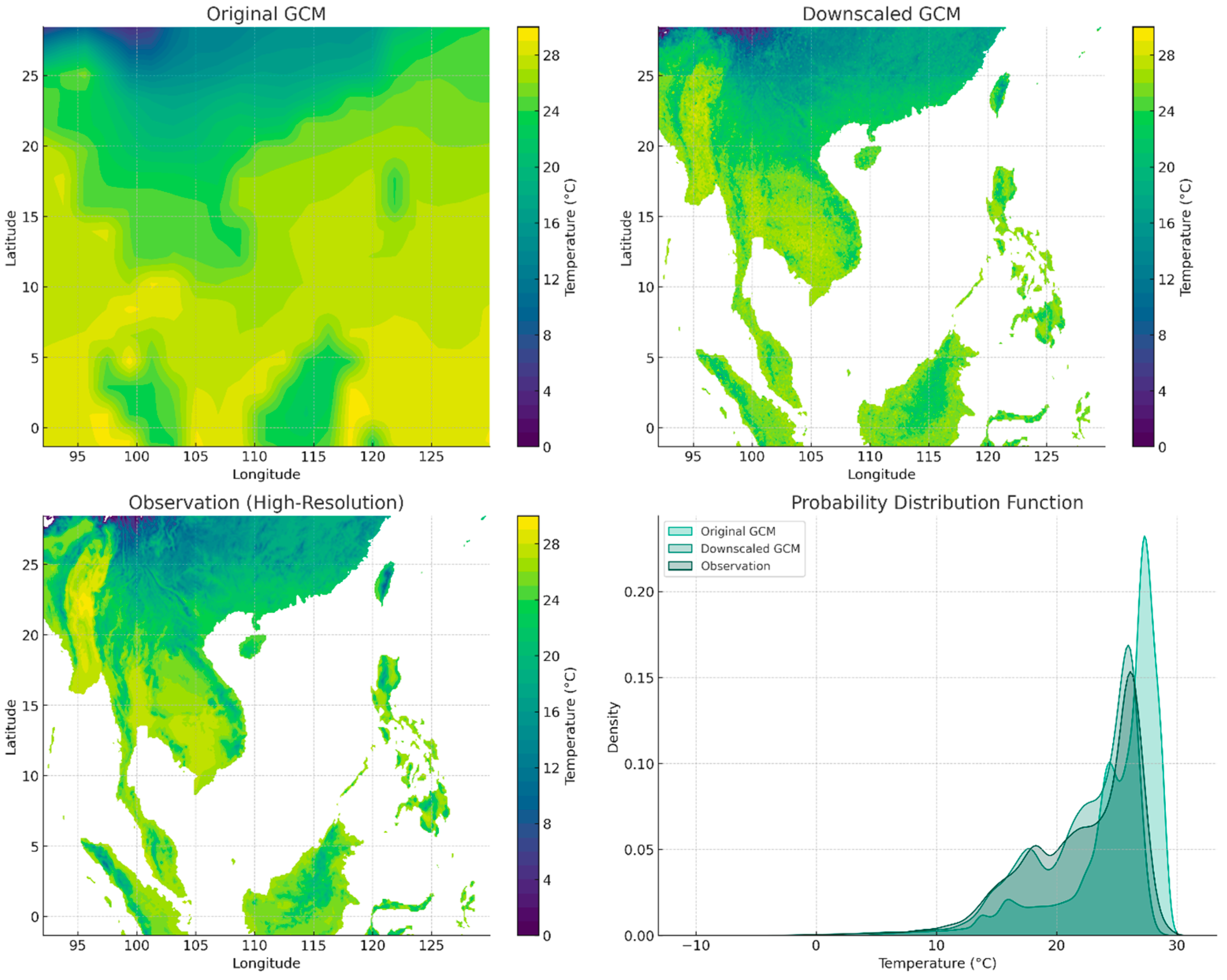
3.1. Random Forest
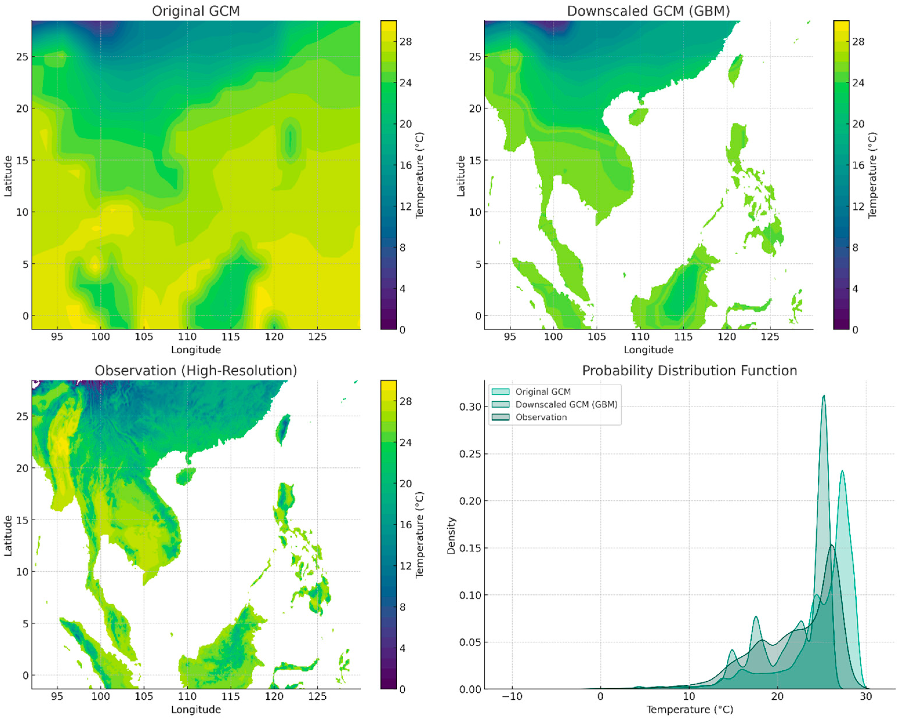
3.2. Gradient Boosting Machine Method
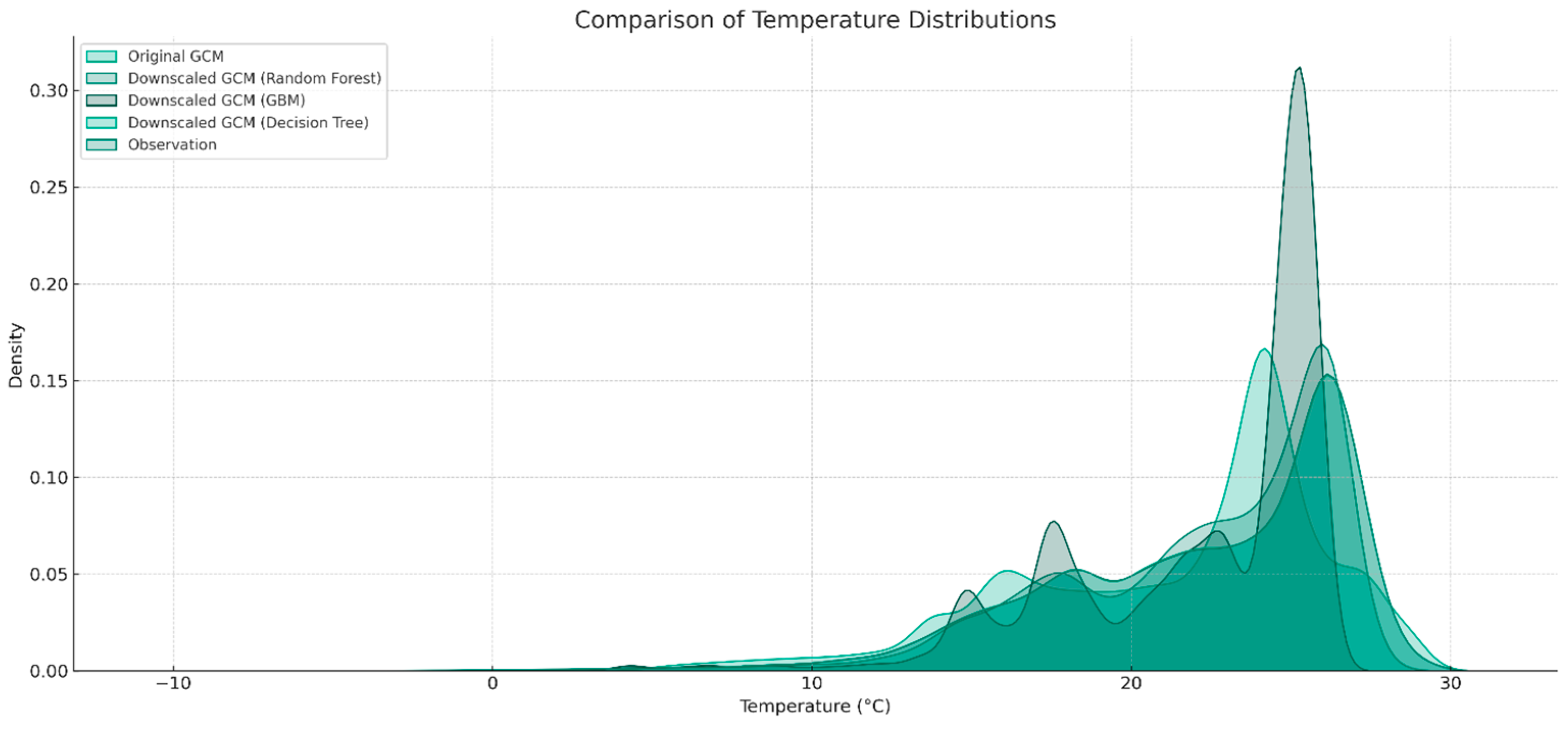
3.3. Decision Tree Learning
4. Discussion
5. Conclusions
Funding
Data Availability Statement
Acknowledgments
Conflicts of Interest
Abbreviations
| SEA | Southeast Asia |
| RF | Random Forest |
| GBM | Gradient Boosting Machine |
| DT | Decision Tree |
| GCM | General Circulation Model |
| MSE | Mean Square Error |
| RMSE | Root Mean Square Error |
| SDR | standard deviation of residuals |
| SVM | Support Vector Machines |
| RCMs | Regional Climate Models |
| ML | Machine Learning |
| CMIP6 | Coupled Model Intercomparison Project Phase 6 |
| MPI-ESM1.2 | Max Planck Institute for Meteorology Earth System Model version 1.2 |
| FEWS NET | Famine Early Warning Systems Network |
| MERRA2 | Modern-Era Retrospective Analysis for Research and Applications version 2 |
| CHIRPS | Climate Hazards Group Infrared Precipitation with Station |
References
- Flato, G.; Marotzke, J.; Abiodun, B.; Braconnot, P.; Chou, S.C.; Collins, W.; Cox, P.; Driouech, F.; Emori, S.; Eyring, V. Evaluation of climate models. In Climate Change 2013: The Physical Science Basis. Contribution of Working Group I to the Fifth Assessment Report of the Intergovernmental Panel on Climate Change; Cambridge University Press: Cambridge, UK, 2014; pp. 741–866. [Google Scholar]
- Pachauri, R.K.; Allen, M.R.; Barros, V.R.; Broome, J.; Cramer, W.; Christ, R.; Church, J.A.; Clarke, L.; Dahe, Q.; Dasgupta, P. Climate Change 2014: Synthesis Report. Contribution of Working Groups I, II and III to the Fifth Assessment Report of the Intergovernmental Panel on Climate Change; IPCC: Paris, France, 2014. [Google Scholar]
- Wilby, R.L.; Charles, S.P.; Zorita, E.; Timbal, B.; Whetton, P.; Mearns, L.O. Guidelines for Use of Climate Scenarios Developed from Statistical Downscaling Methods; Supporting Material of the Intergovernmental Panel on Climate Change; DDC of IPCC TGCIA: Hamburg, Germany, 2004; Volume 27. [Google Scholar]
- Fowler, H.J.; Blenkinsop, S.; Tebaldi, C. Linking climate change modelling to impacts studies: Recent advances in downscaling techniques for hydrological modelling. Int. J. Climatol. A J. R. Meteorol. Soc. 2007, 27, 1547–1578. [Google Scholar] [CrossRef]
- Amnuaylojaroen, T. Air Pollution Modeling in Southeast Asia—An Overview. In Vegetation Fires and Pollution in Asia; Springer: Cham, Switzerland, 2023; pp. 531–544. [Google Scholar]
- Amnuaylojaroen, T.; Chanvichit, P. Projection of near-future climate change and agricultural drought in Mainland Southeast Asia under RCP8. 5. Clim. Chang. 2019, 155, 175–193. [Google Scholar] [CrossRef]
- Amnuaylojaroen, T.; Macatangay, R.C.; Khodmanee, S. Modeling the effect of VOCs from biomass burning emissions on ozone pollution in upper Southeast Asia. Heliyon 2019, 5, e02661. [Google Scholar] [CrossRef]
- Amnuaylojaroen, T.; Surapipith, V.; Macatangay, R.C. Projection of the near-future PM2. 5 in Northern Peninsular Southeast Asia under RCP8.5. Atmosphere 2022, 13, 305. [Google Scholar] [CrossRef]
- Maraun, D.; Wetterhall, F.; Ireson, A.; Chandler, R.; Kendon, E.; Widmann, M.; Brienen, S.; Rust, H.; Sauter, T.; Themeßl, M. Precipitation downscaling under climate change: Recent developments to bridge the gap between dynamical models and the end user. Rev. Geophys. 2010, 48, 1–38. [Google Scholar] [CrossRef]
- Ghosh, S.; Mujumdar, P.P. Statistical downscaling of GCM simulations to streamflow using relevance vector machine. Adv. Water Resour. 2008, 31, 132–146. [Google Scholar] [CrossRef]
- Giorgi, F.; Mearns, L.O. Introduction to special section: Regional climate modeling revisited. J. Geophys. Res. Atmos. 1999, 104, 6335–6352. [Google Scholar] [CrossRef]
- Ghosh, S.; Mujumdar, P. Future rainfall scenario over Orissa with GCM projections by statistical downscaling. Curr. Sci. 2006, 90, 396–404. [Google Scholar]
- Diaz-Nieto, J.; Wilby, R.L. A comparison of statistical downscaling and climate change factor methods: Impacts on low flows in the River Thames, United Kingdom. Clim. Chang. 2005, 69, 245–268. [Google Scholar] [CrossRef]
- Minville, M.; Brissette, F.; Leconte, R. Uncertainty of the impact of climate change on the hydrology of a nordic watershed. J. Hydrol. 2008, 358, 70–83. [Google Scholar] [CrossRef]
- Piccolroaz, S.; Zhu, S.; Ptak, M.; Sojka, M.; Du, X. Warming of lowland Polish lakes under future climate change scenarios and consequences for ice cover and mixing dynamics. J. Hydrol. Reg. Stud. 2021, 34, 100780. [Google Scholar] [CrossRef]
- Cannon, A.J.; Sobie, S.R.; Murdock, T.Q. Bias correction of GCM precipitation by quantile mapping: How well do methods preserve changes in quantiles and extremes? J. Clim. 2015, 28, 6938–6959. [Google Scholar] [CrossRef]
- Bedia, J.; Herrera, S.; Gutiérrez, J.M. Dangers of using global bioclimatic datasets for ecological niche modeling. Limitations for future climate projections. Glob. Planet. Chang. 2013, 107, 1–12. [Google Scholar] [CrossRef]
- Asadollah, S.B.H.S.; Sharafati, A.; Shahid, S. Application of ensemble machine learning model in downscaling and projecting climate variables over different climate regions in Iran. Environ. Sci. Pollut. Res. 2022, 29, 17260–17279. [Google Scholar] [CrossRef]
- Vandal, T.; Kodra, E.; Ganguly, S.; Michaelis, A.; Nemani, R.; Ganguly, A.R. Deepsd: Generating high resolution climate change projections through single image super-resolution. In Proceedings of the 23rd ACM Sigkdd International Conference on Knowledge Discovery and Data Mining, Halifax, NS, Canada, 13–17 August 2017; pp. 1663–1672. [Google Scholar]
- Palmer, T.; Doblas-Reyes, F.; Weisheimer, A.; Rodwell, M. Toward seamless prediction: Calibration of climate change projections using seasonal forecasts. Bull. Am. Meteorol. Soc. 2008, 89, 459–470. [Google Scholar] [CrossRef]
- Reichstein, M.; Camps-Valls, G.; Stevens, B.; Jung, M.; Denzler, J.; Carvalhais, N.; Prabhat, F. Deep learning and process understanding for data-driven Earth system science. Nature 2019, 566, 195–204. [Google Scholar] [CrossRef]
- Lguensat, R.; Tandeo, P.; Ailliot, P.; Pulido, M.; Fablet, R. The analog data assimilation. Mon. Weather. Rev. 2017, 145, 4093–4107. [Google Scholar] [CrossRef]
- Gentine, P.; Pritchard, M.; Rasp, S.; Reinaudi, G.; Yacalis, G. Could machine learning break the convection parameterization deadlock? Geophys. Res. Lett. 2018, 45, 5742–5751. [Google Scholar] [CrossRef]
- Lal, R. Advancing climate change mitigation in agriculture while meeting global sustainable development goals. Soil Water Conserv. A Celebr. 2020, 75, 12–31. [Google Scholar]
- Stocker, T.F.; Qin, D.; Plattner, G.-K.; Tignor, M.M.; Allen, S.K.; Boschung, J.; Nauels, A.; Xia, Y.; Bex, V.; Midgley, P.M. Climate Change 2013: The Physical Science Basis. In Working Group I Contribution to the Fifth Assessment Report of the Intergovernmental Panel on Climate Change; Cambridge University Press: Cambridge, UK, 2014. [Google Scholar]
- Dell, M.; Jones, B.F.; Olken, B.A. Temperature shocks and economic growth: Evidence from the last half century. Am. Econ. J. Macroecon. 2012, 4, 66–95. [Google Scholar] [CrossRef]
- Trenberth, K. Observation: Surface and atmospheric climate change. Climate Change 2007: The Physical Science Basis. In Contribution of Working Group I to the Fourth Assessment Report of the Intergovernmental Panel on Climate Change; Cambridge University Press: Cambridge, UK, 2007. [Google Scholar]
- Villafuerte, M.Q.; Matsumoto, J. Significant influences of global mean temperature and ENSO on extreme rainfall in Southeast Asia. J. Clim. 2015, 28, 1905–1919. [Google Scholar] [CrossRef]
- Maier-Reimer, E.; Hasselmann, K.; Olbers, D.; Willebrand, J. An Ocean Circulation Model for Climate Studies; The Max-Planck-Institut für Meteorologie: Hamburg, Germany, 1982. [Google Scholar]
- Roeckner, E.; Dümenil, L.; Kirk, E.; Lunkeit, F.; Ponater, M.; Rockel, B.; Sausen, R.; Schlese, U. The Hamburg version of the ECMWF model (ECHAM). Research activities in atmospheric and oceanic modelling. CAS/JSC Work. Group Numer. Exp. 1989, 13, 7.1–7.4. [Google Scholar]
- Giorgetta, M.A.; Jungclaus, J.; Reick, C.H.; Legutke, S.; Bader, J.; Böttinger, M.; Brovkin, V.; Crueger, T.; Esch, M.; Fieg, K. Climate and carbon cycle changes from 1850 to 2100 in MPI-ESM simulations for the Coupled Model Intercomparison Project phase 5. J. Adv. Model. Earth Syst. 2013, 5, 572–597. [Google Scholar] [CrossRef]
- Craig, A.; Valcke, S.; Coquart, L. Development and performance of a new version of the OASIS coupler, OASIS3-MCT_3.0. Geosci. Model Dev. 2017, 10, 3297–3308. [Google Scholar] [CrossRef]
- McNally, A.; Jacob, J.; Arsenault, K.; Slinski, K.; Sarmiento, D.P.; Hoell, A.; Pervez, S.; Rowland, J.; Budde, M.; Kumar, S. A Central Asia hydrologic monitoring dataset for food and water security applications in Afghanistan. In Earth System Science Data; Copernicus Publications: Enschede, The Netherlands, 2022; Volume 14. [Google Scholar]
- Adeli, H. Neural networks in civil engineering: 1989–2000. Comput.-Aided Civ. Infrastruct. Eng. 2001, 16, 126–142. [Google Scholar] [CrossRef]
- Obregon, J.; Jung, J.-Y. RuleCOSI+: Rule extraction for interpreting classification tree ensembles. Inf. Fusion 2023, 89, 355–381. [Google Scholar] [CrossRef]
- Mamalakis, A.; Ebert-Uphoff, I.; Barnes, E.A. Explainable artificial intelligence in meteorology and climate science: Model fine-tuning, calibrating trust and learning new science. In Proceedings of the International Workshop on Extending Explainable AI Beyond Deep Models and Classifiers, Vienna, Austria, 17 July 2020; pp. 315–339. [Google Scholar]
- Breiman, L. Random forests. Mach. Learn. 2001, 45, 5–32. [Google Scholar] [CrossRef]
- Friedman, J.H. Greedy function approximation: A gradient boosting machine. Ann. Stat. 2001, 29, 1189–1232. [Google Scholar] [CrossRef]
- Quinlan, J.R. Induction of decision trees. Mach. Learn. 1986, 1, 81–106. [Google Scholar] [CrossRef]
- Bergstra, J.; Bengio, Y. Random search for hyper-parameter optimization. J. Mach. Learn. Res. 2012, 13, 281–305. [Google Scholar]
- Kohavi, R. A study of cross-validation and bootstrap for accuracy estimation and model selection. In Proceedings of the Fourteenth International Joint Conference on Artificial Intelligence, Montreal, QC, Canada, 20–25 August 1995; pp. 1137–1145. [Google Scholar]
- Arlot, S.; Celisse, A. A survey of cross-validation procedures for model selection. Statist. Surv. 2010, 4, 40–79. [Google Scholar] [CrossRef]
- Chai, T.; Draxler, R.R. Root mean square error (RMSE) or mean absolute error (MAE). Geosci. Model Dev. Discuss. 2014, 7, 1525–1534. [Google Scholar]
- Hastie, T.; Tibshirani, R.; Friedman, J.H.; Friedman, J.H. The Elements of Statistical Learning: Data Mining, Inference, and Prediction; Springer: Berlin/Heidelberg, Germany, 2009; Volume 2. [Google Scholar]
- McKinney, W. Data structures for statistical computing in python. In Proceedings of the 9th Python in Science Conference, Austin, TX, USA, 28 June–3 July 2010; pp. 51–56. [Google Scholar]
- Pang, B.; Yue, J.; Zhao, G.; Xu, Z. Statistical downscaling of temperature with the random forest model. Adv. Meteorol. 2017, 2017, 726517. [Google Scholar] [CrossRef]
- Shen, Z.; Yong, B. Downscaling the GPM-based satellite precipitation retrievals using gradient boosting decision tree approach over Mainland China. J. Hydrol. 2021, 602, 126803. [Google Scholar] [CrossRef]
- Ray, P.A.; Taner, M.Ü.; Schlef, K.E.; Wi, S.; Khan, H.F.; Freeman, S.S.G.; Brown, C.M. Growth of the decision tree: Advances in bottom-up climate change risk management. JAWRA J. Am. Water Resour. Assoc. 2019, 55, 920–937. [Google Scholar] [CrossRef]
- Dey, A.; Sahoo, D.P.; Kumar, R.; Remesan, R. A multimodel ensemble machine learning approach for CMIP6 climate model projections in an Indian River basin. Int. J. Climatol. 2022, 42, 9215–9236. [Google Scholar] [CrossRef]
- Behnke, R.; Vavrus, S.; Allstadt, A.; Albright, T.; Thogmartin, W.E.; Radeloff, V.C. Evaluation of downscaled, gridded climate data for the conterminous United States. Ecol. Appl. 2016, 26, 1338–1351. [Google Scholar] [CrossRef] [PubMed]
- Lotfirad, M.; Esmaeili-Gisavandani, H.; Adib, A. Drought monitoring and prediction using SPI, SPEI, and random forest model in various climates of Iran. J. Water Clim. Chang. 2022, 13, 383–406. [Google Scholar] [CrossRef]
- Johnson, J.B.; Omland, K.S. Model selection in ecology and evolution. Trends Ecol. Evol. 2004, 19, 101–108. [Google Scholar] [CrossRef]
- Liaw, A.; Wiener, M. Classification and regression by randomForest. R News 2002, 2, 18–22. [Google Scholar]
- Elith, J.; Leathwick, J.R.; Hastie, T. A working guide to boosted regression trees. J. Anim. Ecol. 2008, 77, 802–813. [Google Scholar] [CrossRef] [PubMed]
- Natekin, A.; Knoll, A. Gradient boosting machines, a tutorial. Front. Neurorobotics 2013, 7, 21. [Google Scholar] [CrossRef] [PubMed]
- Breiman, L. Classification and Regression Trees; Routledge: London, UK, 2017. [Google Scholar]
- Dietterich, T.G. An experimental comparison of three methods for constructing ensembles of decision trees: Bagging, boosting, and randomization. Mach. Learn. 2000, 40, 139–157. [Google Scholar] [CrossRef]
- Cutler, D.R.; Edwards, T.C., Jr.; Beard, K.H.; Cutler, A.; Hess, K.T.; Gibson, J.; Lawler, J.J. Random forests for classification in ecology. Ecology 2007, 88, 2783–2792. [Google Scholar] [CrossRef]
- Dang, L.; Li, J.; Bai, X.; Liu, M.; Li, N.; Ren, K.; Cao, J.; Du, Q.; Sun, J. Novel Prediction Method Applied to Wound Age Estimation: Developing a Stacking Ensemble Model to Improve Predictive Performance Based on Multi-mRNA. Diagnostics 2023, 13, 395. [Google Scholar] [CrossRef]


| Method | MSE | Pearson Correlation | Standard Deviations of the Residuals | MB |
|---|---|---|---|---|
| Random Forest (RF) | 2.78 | 0.94 | 1.67 | −0.0079 |
| Gradient Boosting Machine (GBM) | 5.90 | 0.86 | 2.43 | −0.0085 |
| Decision Tree (DT) | 2.43 | 0.95 | 1.56 | −0.0046 |
| Original GCM | 7.84 | 0.84 | 2.74 | −0.6512 |
Disclaimer/Publisher’s Note: The statements, opinions and data contained in all publications are solely those of the individual author(s) and contributor(s) and not of MDPI and/or the editor(s). MDPI and/or the editor(s) disclaim responsibility for any injury to people or property resulting from any ideas, methods, instructions or products referred to in the content. |
© 2023 by the author. Licensee MDPI, Basel, Switzerland. This article is an open access article distributed under the terms and conditions of the Creative Commons Attribution (CC BY) license (https://creativecommons.org/licenses/by/4.0/).
Share and Cite
Amnuaylojaroen, T. Advancements in Downscaling Global Climate Model Temperature Data in Southeast Asia: A Machine Learning Approach. Forecasting 2024, 6, 1-17. https://doi.org/10.3390/forecast6010001
Amnuaylojaroen T. Advancements in Downscaling Global Climate Model Temperature Data in Southeast Asia: A Machine Learning Approach. Forecasting. 2024; 6(1):1-17. https://doi.org/10.3390/forecast6010001
Chicago/Turabian StyleAmnuaylojaroen, Teerachai. 2024. "Advancements in Downscaling Global Climate Model Temperature Data in Southeast Asia: A Machine Learning Approach" Forecasting 6, no. 1: 1-17. https://doi.org/10.3390/forecast6010001