Article

A Monte Carlo Approach to Bitcoin Price Prediction with Fractional Ornstein–Uhlenbeck Lévy Process

by
Jules Clément Mba
1,*,
Sutene Mwambetania Mwambi
1 and
Edson Pindza
2,3
1
School of Economics, College of Business and Economics, University of Johannesburg, P.O. Box 524 Auckland Park, Johannesburg 2006, South Africa
2
Department of Mathematics and Statistics, Tshwane University of Technology, Pretoria 0001, South Africa
3
Department of Mathematics and Applied Mathematics, University of Pretoria, Pretoria 0002, South Africa
*
Author to whom correspondence should be addressed.
Forecasting 2022, 4(2), 409-419; https://doi.org/10.3390/forecast4020023
Submission received: 26 February 2022 / Revised: 20 March 2022 / Accepted: 24 March 2022 / Published: 30 March 2022

Abstract

:
Since its inception in 2009, Bitcoin has increasingly gained main stream attention from the general population to institutional investors. Several models, from GARCH type to jump-diffusion type, have been developed to dynamically capture the price movement of this highly volatile asset. While fitting the Gaussian and the Generalized Hyperbolic and the Normal Inverse Gaussian (NIG) distributions to log-returns of Bitcoin, NIG distribution appears to provide the best fit. The time-varying Hurst parameter for Bitcoin price reveals periods of randomness and mean-reverting type of behaviour, motivating the study in this paper through fractional Ornstein–Uhlenbeck driven by a Normal Inverse Gaussian Lévy process. Features such as long-range memory are jump diffusion processes that are well captured with this model. The results present a 95% prediction for the price of Bitcoin for some specific dates. This study contributes to the literature of Bitcoin price forecasts that are useful for Bitcoin options traders.
JEL Classification:
C15; C53; G17

1. Introduction

Cryptocurrency is a digital currency that uses advanced encryption techniques known as cryptography to secure financial transactions, control the creation of additional units, and verify the transfer of assets. It uses decentralized control by using distributed ledger technology called Blockchain, which serves as a public financial transaction database. Bitcoin is the first decentralized cryptocurrency introduced in 2009 by a person or a group of persons under the pseudonym Sathoshi Nakamoto [1]. Many other alternatives of Bitcoin have been created. On Coinmarketcap (https://coinmarketcap.com/, accessed on 25 February 2022), there are 2322 tradable cryptocurrencies with a total market capitalization of USD 345 billions at the time of this paper (see [2,3] for further background on the Bitcoin and its technology). The cryptocurrency market is known to be highly volatile [4,5,6,7] due, on the one hand, to its sensibility to new information, whether fundamental or speculative [8], since it does not rely on the stabilizing policy of a central bank. On the other hand, the relative liquidity of the market with no official market makers makes it fundamentally fragile to large trading volumes and to market imperfections; thus, it is more prone to large swings than other traded assets (see [9]). In such environments, suitable forecasting models for cryptocurrencies have to reflect all these underlying features. Bitcoin prices have been already modeled and predicted by means of a noncausal autoregressive process [10], fractional geometric Brownian motion [11], and machine learning [12,13] to name the few. Andrew and Christian [10] applied the noncausal autoregressive process with Cauchy errors to model and predict Bitcoin prices. Their results display episodes of local trends, which can be modeled and interpreted as speculative bubbles. Tarnopolski [11] used the fractional geometric Brownian motion to account for the long-memory or long-term dependence of Bitcoin (BTC), manifesting itself through a Hurst exponent H > 0.5 , in order to predict future BTC/USD price. To achieve this, a Monte Carlo simulation with 10 4 geometric fractional Brownian motion realizations was performed as extensions of historical data, and the accuracy of statistical inferences is taken to be 10%. Tarnopolski [11] concluded the prediction that the most probable Bitcoin prices at the beginning of 2018 will be 6358 USD. Jalali and Heidari [14] predicted the price of Bitcoin and changes therein using a first-order Grey model (GM (1,1)). Other studies on cryptocurrency prediction using variants of Grey models can be found in Gatabazi et al. [15,16,17]. However, the grey system theory prediction works better only with small size datasets, as the error of prediction will increase as the dataset becomes larger (Wu et al. [18]). Moreover, small size dataset does not exhibit some of the important characteristics of the data, such as long range dependence as well as the size and frequency of jumps. McNally et al. ascertained information on what accuracy the direction of Bitcoin price can be predicted. This task is achieved with varying degrees of success through the implementation of a Bayesian optimized recurrent neural network (RNN) and a Long Short Term Memory (LSTM) network. They showed that these non-linear deep learning methods outperform the popular ARIMA model for time series forecasting. As shown by Jalali and Heidari [14], these neural network models are sensitive to input variables, given that the Bitcoin price depends on different inputs with complex behaviors, as illustrated by Chen et al. [19] and Kristoufek and Ladislav [20]. Based on new technologies, economic policies, and cultural behaviors, these inputs may change. Motivated by these shortcomings, we introduce a mean-reverting fractional jump-diffusion stochastic model in this study to predict Bitcoin exchange rates.
Since Bitcoin exchange rates not only exhibit long-range dependence [21], they also present some periods of randomness and mean-reverting feature. Moreover, they exhibit abrupt and discontinuous changes in prices known as jumps, which are assumed to follow some probability law [9]. We present in this paper a fractional Ornstein–Uhlenbeck driven by a Normal Inverse Gaussian Lévy process for short-term predictions of Bitcoin exchange rates.
The rest of the paper is organized as follows: Section 2 introduces the methodology used, Section 3 discusses the empirical findings, and the last Section concludes the study.

2. Materials and Methods

In this section, the basic structure of the fractional Ornstein–Uhlenbeck Lévy (fOUL) model is described where the Bitcoin price process at any time point t, { X t } t 0 is modeled as an exponential of a Lévy process. The model augments two continuous-time random processes: a fractional Brownian process and a compound Poisson jump process, which also generates two random sources. Fractional Brownian motion could be divided into three different categories:
  • The process is likely to reverse the trend over the time frame considered.
  • The process is random in which knowing one data point does not provide insight into predicting future data points.
  • The process is persistent in the sense that a future data point is likely to be similar to a data point preceding it.
This is of particular importance in examining long-range dependence in processes. The below subsection presents some details of the a fractional Brownian motion.

2.1. Fractional Brownian Motion

For a normalized (i.e., E [ B H ( 1 ) 2 ] ) fractional Brownian motion B H ( t ) , define the incremental process B = { b H ( k ) : k = 0 , 1 , } , which is also called fractional Gaussian noise, by the following.
b H ( k ) = B H ( k + 1 ) B H ( k ) .
The increments ( b H ( k ) ) follow a standard normal distribution with zero mean and variance E [ b H ( k ) 2 ] = E [ ( B H ( k + 1 ) B H ( k ) ) 2 ] = E [ B H ( 1 ) 2 ] = 1 , but there is no independence. The corresponding autocovariance function γ H ( · ) is of the following form.
γ H ( k ) = 1 2 [ | k 1 | 2 H 2 | k | 2 H + | k + 1 | 2 H ] , k Z .
If H = 1 2 , all the covariances are zero (except for k = 0 ), implying independence. This is in agreement with the standard Brownian motion, which has independent increments. Using the Taylor expansion at the origin of the function h ( x ) = ( 1 x ) 2 H 2 + ( 1 + x ) 2 H , one has γ H ( k ) = 1 2 k 2 H h ( 1 / k ) for k 1 .
In particular, we have the following.
lim k γ H ( k ) H ( 2 H 1 ) k 2 H 2 = 1
Therefore, the following is the case.
k = 1 γ H ( k ) = , for H > 1 2 ;
k = 1 | γ H ( k ) | < , for H < 1 2 .
Hence, only in the case of H > 1 2 , fractional Brownian motions display long-memory dependence.
For a fixed real number H ( 1 2 , 1 ) , let { B t H , t 0 } be a fractional Brownian motion (fBm) with Hurst parameter H on a complete probability space ( Ω , F , P ) . The integral with respect to B H in the generalized sense of Lebesgue–Stieltjes is defined using the fractional derivatives for a < b and α ( 0 , 1 ) as follows.
( D a + α f ) ( x ) = 1 Γ ( 1 α ) f ( x ) ( x a ) α + α a x f ( x ) f ( u ) ( x u ) 1 + α d u
( D b 1 α g ) ( x ) = e i π α Γ ( α ) g ( x ) ( b x ) 1 α + ( 1 α ) x b g ( x ) g ( u ) ( u x ) 2 α d u
Provided that D a + α f L 1 [ a , b ] , D b 1 α g b L [ a , b ] , where g b ( x ) = g ( x ) g ( b ) . The generalized Lebesgue–Stieltjes integral a b f ( x ) d g ( x ) is given by the following.
a b f ( x ) d g ( x ) = e i π α a b ( D a + α f ) ( x ) ( D b 1 α g b ) ( x )
From the H o ¨ lder continuity of B H , it follows that, for α ( 1 H , 1 ) , D b 1 α B b H L [ a , b ] a.s. Then, for a function f with D a + α f L 1 [ a , b ] , the integral with respect to B H can be defined as follows.
a b f ( x ) d B H ( x ) = e i π α a b ( D a + α f ) ( x ) ( D b 1 α B b H ) ( x )
The tracking of the variation of the Hurst parameter H Figure 1 suggests a mean-reverting process for the data (since H < 1 / 2 for a large part of the time period). This justifies our choice for a fractional Ornstein–Uhlenbeck Lévy process. Let us start by defining a Lévy process. A Lévy process L = ( L t ) t 0 can be decomposed into a Brownian motion W = ( W t ) t 0 and a pure jump process Z = ( Z t ) t 0 independent from the Brownian motion as follows.
L t = σ W t + Z t
The building block of the pure jump process Z is the Poisson process.
While fitting the Normal, Hyperbolic, Generalized Hyperbolic, and Normal Inverse Gaussian (NIG) distributions to the log returns of Bitcoin data (see Figure 2), NIG displays the best fit. We consider, in this work, the fractional Ornstein–Uhlenbeck Lévy process where the jump part is modeled by an NIG process. Before presenting this model, it is important to recall what a Levy process as well as the Normal Inverse Gaussian distribution are.

2.2. Lévy Process

2.2.1. Infinitely Divisible Distributions

A random variable X is called infinitely divisible, if for each positive integer n 2 , there exist independent and identically distributed (i.i.d) random variables X 1 , X 2 , , X n such that the distribution of Y is the same as the distribution of k = 1 n X k and has a characteristic function. In the literature, the characteristic function of the one-dimensional infinitely divisible distribution is generalized by the Lévy–Khinchin–Kolmogorov formula given below.
Let us start by defining the cumulative generating function of the random vector x = ( x 1 , , x n ) R n , which determines the Lévy measure.
The p th order joint cumulant of x is given by the following:
cum ( x ) = ( 1 ) k 1 ( k 1 ) ! ( E r p 1 x r ) ( E r p k x r ) ,
where E is the expectation operator, and the summation extends over all partitions ( p 1 , , p k ) , k = 1 , , n , of ( 1 , , n ) . Note that cum ( x ) is the coefficient of i n ξ 1 ξ n in the Taylor series expansion about the origin of the following function, known as the cumulant generating function of the random vector x .
C ( ξ , x ) = l o g E [ e x p ( i r = 1 n ξ r x r ) ] , x = ( x 1 , , x n ) , ξ = ( ξ 1 , , ξ n ) R n ,
If function C ( ξ , x ) has the following Lévy–Khinchin–Kolmogorov form:
C ( ξ , x ) = i a ξ b ξ 2 2 + κ ( ξ ) , ξ R
then the random variable x follows an infinitely divisible distribution, where the following is the case: a , b R , b 0 ,
κ ( ξ ) = R ( exp i ξ v 1 i ξ ϕ ( v ) ) Q ( d v ) , ξ R
and Q is a Radon measure on R with the following:
Q ( 0 ) = 0 , R min ( 1 , v 2 ) Q ( d v ) < ,
and where function ϕ in Equation (4) is of the following form.
ϕ ( v ) = v , if | v | 1 , v | v | , if | v | > 1
The measure Q in Equation (4) is called the Lévy measure of x . The variable a is referred to as the center or drift and determines the location, and b is the variance. The Lévy triplet ( a , b , Q ) determines x uniquely. If b = 0 , then the distribution is referred to as a purely non-Gaussian distribution.
Examples of infinitely divisible distributions include Normal (Gaussian), Poisson, Gamma, Variance Gamma (VG), and Inverse Gamma (IG) distributions, to name the few. Their corresponding Lévy measures are Q G a u s s i a n ( d x ) = 0 , Q P o i s s o n ( d x ) = λ δ λ ( d x ) , Q G a m m a ( d x ) = c e λ x x 1 x > 0 d x , Q V G ( d x ) = ( c e λ + x x 1 x > 0 + c e λ | x | x 1 x < 0 ) d x , and Q I G ( d x ) = c e λ 2 2 x 2 π x 3 2 1 x > 0 d x , respectively. The Poisson, gamma, VG, and IG distributions are purely non-Gaussian distributions.

2.2.2. Continuous-Time Stochastic Processes

Using infinitely divisible distributions, one can define a continuous sequence of independently infinitely divisible random variables, which will be referred to as the continuous-time stochastic processes. The two basic classes of continuous-time stochastic processes are Brownian motion and the Poisson process. The Poisson process generated by the Poisson distribution is the building block of pure jump processes. Both processes are fundamentally different concerning their path properties and the fact that they belong to the larger class of Lévy processes (for more details about Lévy processes, see [5]. Cont and Tankov [6] provide details of Lévy processes with applications to finance). A stochastic process X = ( X t ) t 0 is a family of R -valued random variables X t with parameter t 0 , defined on the sample space Ω .
A real-valued stochastic process L = { L t , t 0 } defined in a complete probability space ( Ω , F , P ) is called a Lévy process if the following is the case:
  • The random variables L t 0 , L t 1 L t 0 , , L t n L t n 1 are independent for all n 1 and 0 t 0 < t 1 < < t n (independent increments);
  • L t + s L t has the same distribution as L s for all s , t 0 (stationary increments);
  • L is stochastically continuous; that is, for all t 0 and a > 0 .
    lim s t P [ | L s L t | > a ] = 0 .
  • The paths t L t are right-continuous with left limits (cadlag-continue á droite et limite á gauche).

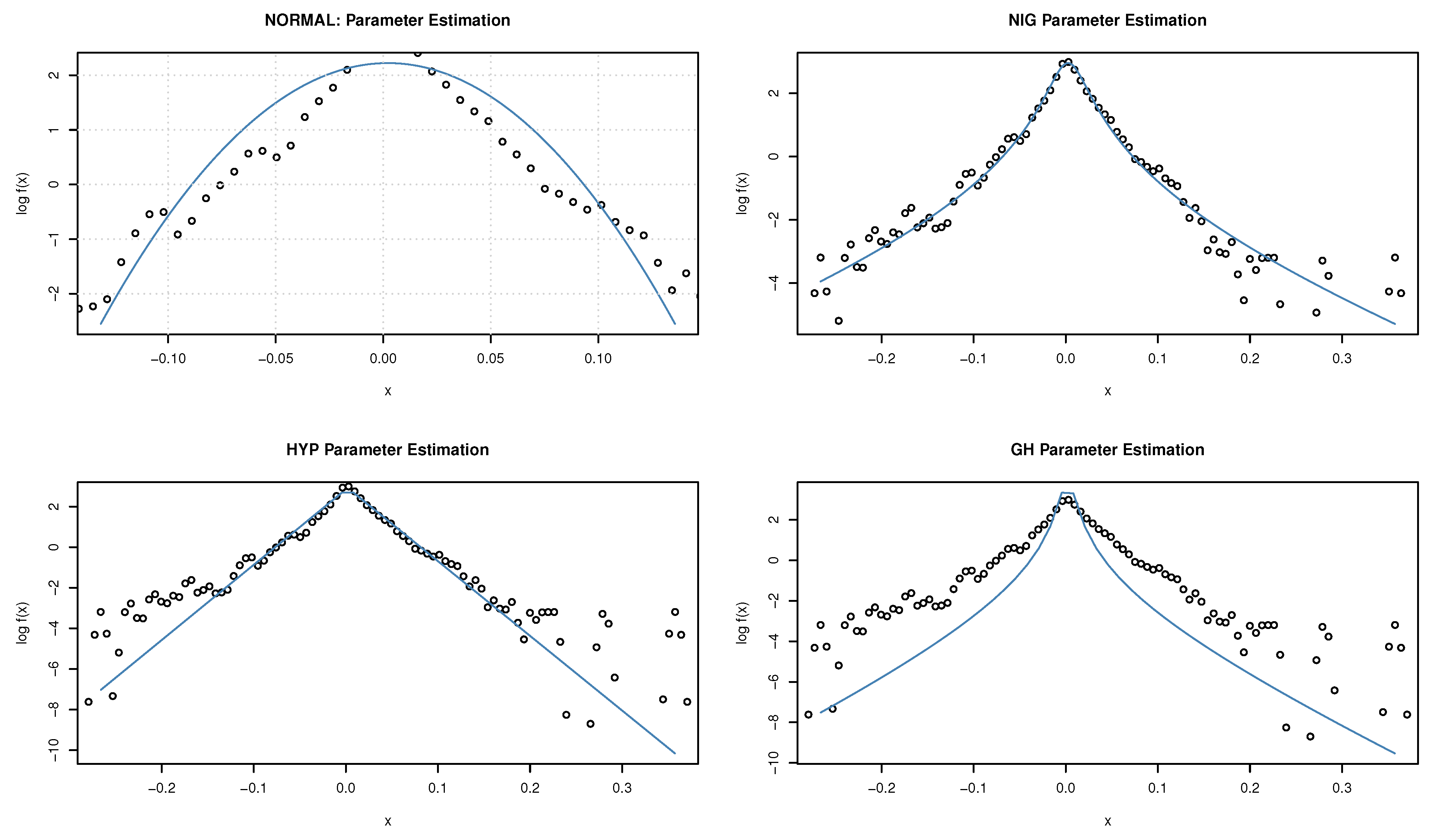
2.2.3. Normal Inverse Gaussian

An N -vlued stochastic process N = ( N t ) t 0 is called a Poisson process with intensity λ ( 0 , ) if N satisfies (i)–(iii) and if the following is the case.
  • iv) P ( N t = k ) = ( λ t ) k k ! exp ( λ t ) , k 0 , t 0 (Poisson distribution).
We can define more general Lévy processes as follows:
C t = k = 1 N t Y k , t 0 ,
for a Poisson process ( N t ) t 0 and independently identically distributed Y k , and with k 1 being the jump size distribution f ( . ) . Such processes are called compound Poisson processes. The characteristic function of C t is given by the following.
ϕ C t ( v ) = exp ( λ t R ( e i v x 1 ) f ( x ) d x ) .
If f is given by the probability density function of the normal distribution, then C = ( C t ) t 0 is referred to as a jump diffusion process. The total intensity of Poisson processes with jump sizes in the interval [ x , x + d x ] is determined by density λ f ( d x ) .
Consider a process X s = ( X t s ) t 0 with X t s = s N t λ ( s ) , where s is a given a real number and ( N t λ ( s ) ) t 0 is the Poisson process with intensity λ ( s ) . The number s represents the jump size, and intensity λ ( s ) is the expected number of jumps with size s in the unit time.
Let S = { s i R : s i 0 , i = 1 , 2 , } be a subset of jump sizes, λ ( s i ) > 0 for all s i S . Consider a process Y = ( Y t ) t 0 defined by the following.
Y t = γ t + i = 1 X t s i .
For process Y, function Q defined for any subset V of S to be Q ( V ) = s i V λ ( s i ) represents the expected number of jumps with size s i V in the unit time interval. Thus, the map Q from a subset of R to R + is a measure. Using Q, we can obtain an extended process Y such that the characteristic function of Y t is given by the following:
ϕ Y t ( v ) = exp ( i γ v t + t R ( e i v x 1 ) Q ( d x ) )
where γ R , and Q is referred to as a Lévy measure, which captures both the discontinuities rate of occurrence and their overall size. The process Y will be called a pure jump process if its characteristic exponent ϕ Y ( v ) ( ϕ Y ( v ) = exp ( ψ Y ( v ) ) , where ψ Y ( v ) is proportional to the time period as ψ Y t ( v ) = t × ψ Y 1 ( v ) ) is of the following form.
ϕ Y t ( v ) = exp t i γ v + R ( e i v x 1 i v x 1 | x | 1 ) Q ( d x ) .
If t = 1 , then we have a purely non-Gaussian infinitely divisible random variable. Thus, there is a one-to-one correspondence between a purely non-Gaussian infinitely divisible random variable and a pure jump process. If a pure jump process T = ( T t ) t 0 is nondecreasing (that is, T t 0 almost surely for t > 0 , and T t T l almost surely for l t ), then process T is called a subordinator or intrinsic time process. The Poisson, gamma, and inverse Gaussian processes are nondecreasing; hence, they are subordinators. By considering the inverse Gaussian process T = ( T t ) t 0 as the subordinator of Brownian motion W = ( W t ) t 0 , we obtain the Normal Inverse Gaussian (NIG) process L = ( L t ) t 0 with the following.
L t = μ T t + σ W T t .
We can now present the model to be used in this study.

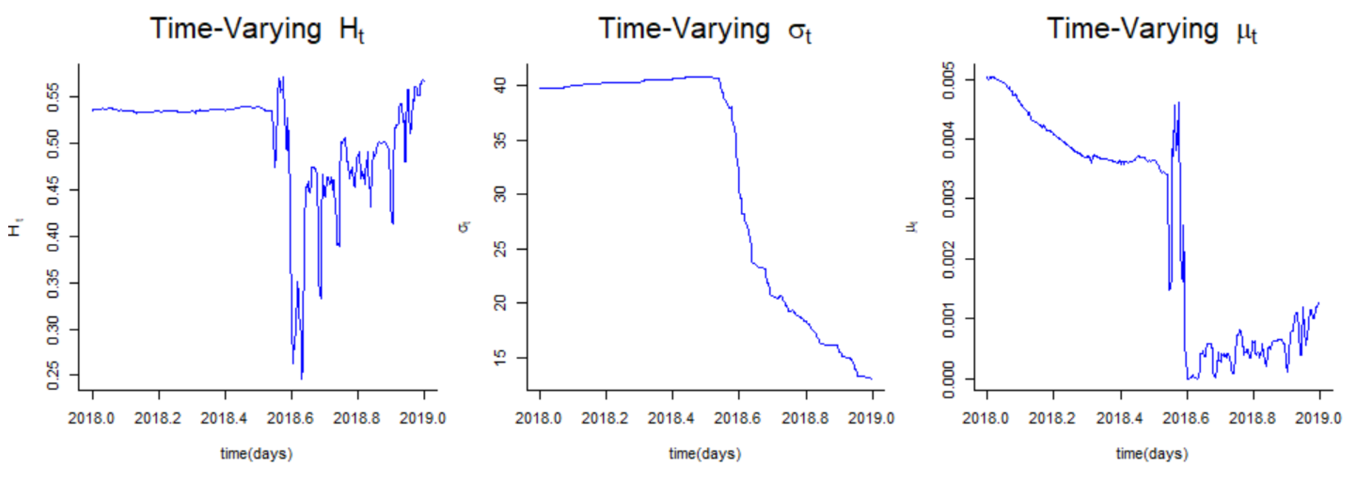
2.3. Fractional Ornstein–Uhlenbeck Lévy Process
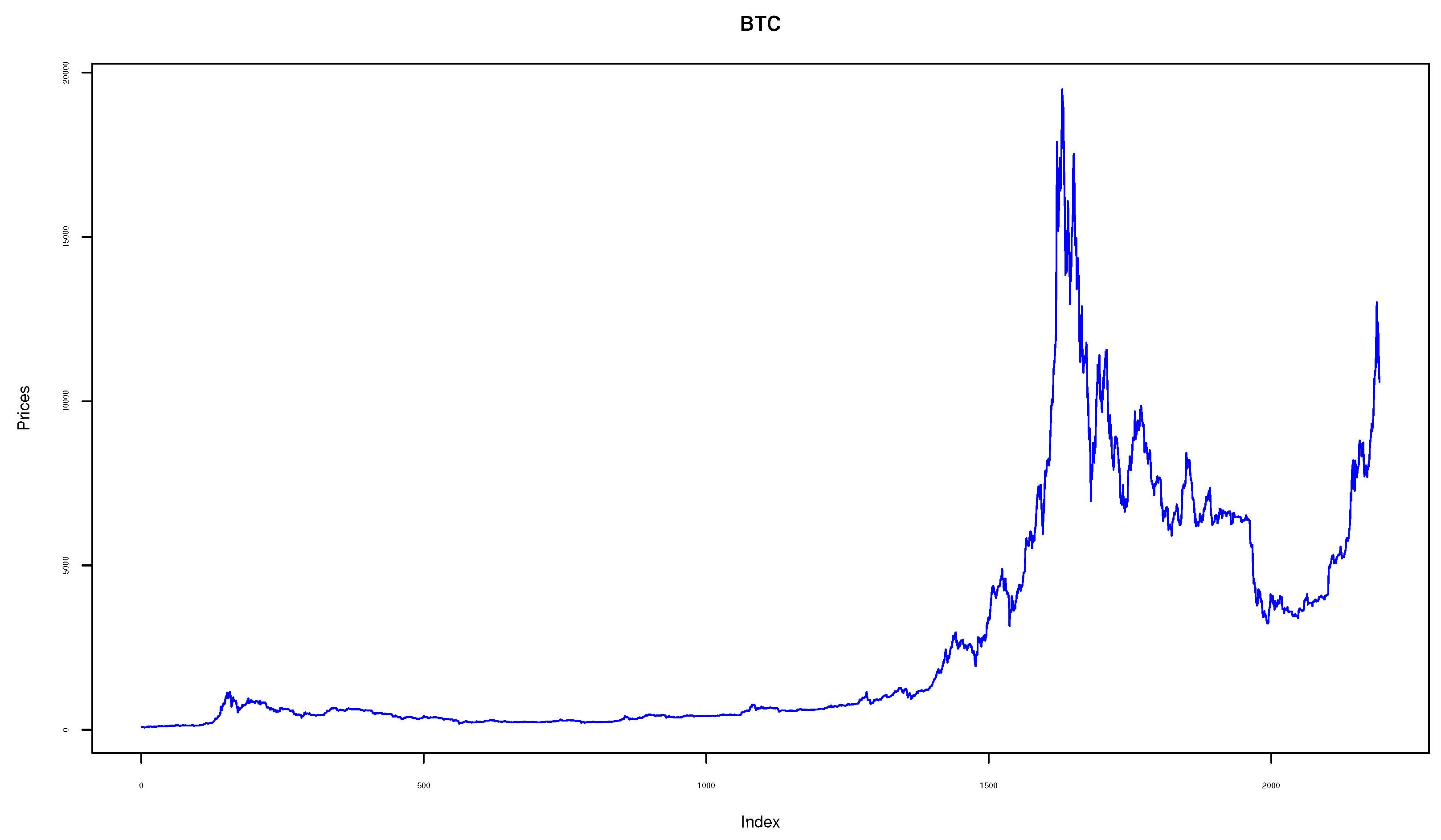
The fractional Ornstein–Uhlenbeck Lévy (fOUL) process X = { X t } t 0 is a solution of the following stochastic differential equation:
d X t = α X t d t + d L t H
where α > 0 is a parameter, and L H = ( L H ) t 0 ) is a fractional NIG Lévy process with Hurst parameter H.
By applying Ito’s formula to function f ( t , X t ) = X t e α t , we obtain the following.
d f ( t , X t ) = e α t d L t H
Thus, the solution of the Equation (7) is given by the following.
X t = X 0 e α t + 0 t e α ( t s ) d L s H
In practice, as the price is observed at fixed times 0 = t 0 < t 1 < t 2 < < t n = T , with constant Δ t = t k + 1 t k , the solution (8) can be discretized by
X t k + 1 = X t k e α Δ t + t k t k + 1 e α ( t k + 1 s ) d L s H .

3. Results

The data comes from the Coinmarketcap website (https://coinmarketcap.com/, accessed on 25 February 2022) and covers a period of 5 years starting from 28 April 2013 to 18 July 2019 with a total of 2283 data points (trading days). The evolution of closing prices S t and the corresponding time paths of logarithmic returns r t series over the study period are depicted in Figure 3. As illustrated, the daily log-returns lie between [ 0.27 , 0.36 ] over the observed period. The plots confirm the presence of volatility clustering and jumps.
Figure 4 depicts a Monte Carlo simulation with 1000 trajectories at equidistant time step t ( 0 , Δ t , 2 Δ t , , T ) where the time step is set at Δ t = 1 and T = 30 .
Figure 4 depicts a Monte Carlo simulation with 1000 trajectories at equidistant time step t ( 0 , Δ t , 2 Δ t , , T ) where the time step is set at Δ t = 1 and T = 30 . This technique is useful in the estimation of the conditional value at risk(CVaR) and most notably in pricing derivatives such as over the counter (OTC) options where market prices are not observable. Other applications have been found in quantifying the extent of mispricings in vanilla options.
Figure 5 is a graphical display of histograms for an empirical distribution superimposed with the best fitting density distribution, which has been taken at specified time points: 29 July 2019, 8 August 2019 and 18 August 2019. Notice that, the shape of the distributions are almost symmetrical apart from the slight skewness in the left tails.

4. Discussion

On one hand, Figure 2 reveals that the Normal Inverse Gaussian (NIG) distributions fits better to the log-returns of data as compared to the Gaussian distribution, Hyperbolic distribution, and Generalized Hyperbolic distribution. This indicates that Bitcoin data are non-Gaussian, and any prediction model with only a Gaussian process may be misleading. Moreover, a stochastic model driven by a Lévy process is more likely to bring reliable forecast results.
On the other hand, given the self-similarity property of Bitcoin, a fractional Brownian motion model will be convenient to simulate its future prices. Tracing the variation of Hurst parameter H estimated from Bitcoin data over a one year (entire 2018) period (see Figure 1) reveals that H remains below 1 / 2 during almost the entire second half of 2018. Thus, we choose the mean-reverting fractional stochastic model, such as the fractional Ornstein–Uhlenbeck stochastic driven by NIG processes for the prediction of Bitcoin’s future prices.
Table 1 is a percentile table that quantifies the risk of the Bitcoin price being above or below a certain level. The economic interpretation of the p-th percentile is the value such that P ( X t x t ) = p α α ( 0.25 ,   0.50 ,   0.75 ,   0.90 ,   0.95 ,   0.99 ) . The 50th percentile is also called the median, whereas the 25th and 75th percentiles are called quantiles. Using the closing price on 19 July, we can easily forecast future prices at specific time intervals: t ( Δ t = 10 d a y ( 29 J u l y ) , Δ t = 20 d a y ( 8 A u g ) and Δ t = 30 d a y ( 18 A u g ) ) .

5. Conclusions

This paper assess bitcoin exchange rate dynamics by using a time-variant Hurst parameter and forecasts its future value by using a fractional Ornstein–Uhlenbeck driven by a Levy process. The time-dependent Hurst parameter H reveals that Bitcoin displays various memory dependency across the study period: mean-revertingness ( H < 1 2 ) , randomness ( H = 1 2 ) , and persistency ( H > 1 2 ) . While fitting the Gaussian, the Hyperbolic, the Generalized Hyperbolic, and the Normal Inverse Gaussian (NIG) distributions to log-returns of bitcoin, the NIG distribution appears to provide the best fit. This justifies our selection of a stochastic model driven by NIG process. As a result, a Monte Carlo simulation through a fractional Ornstein–Uhlenbeck driven by the NIG process predicts that there is a 95% chance for Bitcoin prices to be less that USD 11,881, USD 12,245, and USD 13,157 on 29 July 2019, 8 August 2019, and 18 August 2019, respectively. This model is interesting in two ways: It captures specific features of bitcoin price movement such as memory dependence and abrupt jumps. It could be of interest to Bitcoin options’ traders.

Author Contributions

Conceptualization, E.P. and J.C.M.; methodology, J.C.M.; software, S.M.M.; validation, E.P., J.C.M. and S.M.M.; formal analysis, J.C.M.; investigation, J.C.M.; data curation, J.C.M.; writing—original draft preparation, J.C.M.; writing—review and editing, E.P. and S.M.M.; visualization, S.M.M. All authors have read and agreed to the published version of the manuscript.

Funding

This research received no external funding.

Data Availability Statement

The data used for this study can be obtained from the authors upon request or visit Coinmarketcap: https://coinmarketcap.com/, accessed on 25 February 2022.

Acknowledgments

This work is dedicated in memory of late Sutene Mwambi who contributed significantly to it. Sutene passed away at the final stage of conclusion of this article.

Conflicts of Interest

The authors declare no conflict of interest.

References

  1. Nakamoto, S. Re: Bitcoin P2P e-cash paper. Email Posted List. 2008, 9, 4. [Google Scholar]
  2. Yermack, D. Is Bitcoin a real currency? An economic appraisal. In Handbook of Digital Currency; Elsevier: Amsterdam, The Netherlands, 2015; pp. 31–43. [Google Scholar]
  3. Yermack, D. Corporate governance and blockchains. Rev. Financ. 2017, 21, 7–31. [Google Scholar] [CrossRef] [Green Version]
  4. Dwyer, G.P. The economics of Bitcoin and similar private digital currencies. J. Financ. Stab. 2015, 17, 81–91. [Google Scholar] [CrossRef] [Green Version]
  5. Ken-Iti, S. Lévy Processes and Infinitely Divisible Distributions; Cambridge University Press: Cambridge, UK, 1999. [Google Scholar]
  6. Cont, R.; Tankov, P. Nonparametric calibration of jump-diffusion option pricing models. J. Comput. Financ. 2004, 7, 1–49. [Google Scholar] [CrossRef] [Green Version]
  7. Katsiampa, P. Volatility estimation for Bitcoin: A comparison of GARCH models. Econ. Lett. 2017, 158, 3–6. [Google Scholar] [CrossRef] [Green Version]
  8. Cheah, E.T.; Fry, J. Speculative bubbles in Bitcoin markets? An empirical investigation into the fundamental value of Bitcoin. Econ. Lett. 2015, 130, 32–36. [Google Scholar] [CrossRef] [Green Version]
  9. Scaillet, O.; Treccani, A.; Trevisan, C. High-frequency jump analysis of the bitcoin market. J. Financ. Econom. 2020, 18, 209–232. [Google Scholar]
  10. Hencic, A.; Gouriéroux, C. Noncausal autoregressive model in application to bitcoin/USD exchange rates. In Econometrics of Risk; Springer: Cham, Switzerland, 2015; pp. 17–40. [Google Scholar]
  11. Tarnopolski, M. Modeling the price of Bitcoin with geometric fractional Brownian motion: A Monte Carlo approach. arXiv 2017, arXiv:1707.03746. [Google Scholar]
  12. McNally, S. Predicting the Price of Bitcoin Using Machine Learning. Ph.D. Thesis, National College of Ireland, Dublin, Ireland, 2016. [Google Scholar]
  13. McNally, S.; Roche, J.; Caton, S. Predicting the price of Bitcoin using Machine Learning. In Proceedings of the 2018 26th Euromicro International Conference on Parallel, Distributed and Network-based Processing (PDP), Cambridge, UK, 21–23 March 2018; pp. 339–343. [Google Scholar]
  14. Jalali, M.F.M.; Heidari, H. Predicting changes in Bitcoin price using grey system theory. Financ. Innov. 2020, 6, 13. [Google Scholar]
  15. Gatabazi, P.; Mba, J.C.; Pindza, E.; Labuschagne, C. Grey Lotka- Volterra models with application to cryptocurrencies adoption. Chaos Solitons Fractals 2019, 122, 47–57. [Google Scholar] [CrossRef]
  16. Gatabazi, P.; Mba, J.C.; Pindza, E. Modeling cryptocurrencies transaction counts using variable-order Fractional Grey Lotka-Volterra dynamical system. Chaos Solitons Fractals 2019, 127, 283–290. [Google Scholar] [CrossRef]
  17. Gatabazi, P.; Mba, J.C.; Pindza, E. Fractional gray Lotka- Volterra models with application to cryptocurrencies adoption. Chaos Interdiscip. J. Nonlinear Sci. 2019, 29, 073116. [Google Scholar] [CrossRef] [PubMed]
  18. Wu, L.; Liu, S.; Yao, L.; Yan, S. The effect of sample size on the grey system model. Appl. Math. Model. 2013, 37, 6577–6583. [Google Scholar] [CrossRef]
  19. Chen, H.; De, P.; Hu, Y.J.; Hwang, B.H. Wisdom of crowds: The value of stock opinions transmitted through social media. Rev. Financ. Stud. 2014, 27, 1367–1403. [Google Scholar] [CrossRef]
  20. Kristoufek, L. What are the main drivers of the Bitcoin price? Evidence from wavelet coherence analysis. PLoS ONE 2015, 10, e0123923. [Google Scholar] [CrossRef] [PubMed]
  21. Lahmiri, S.; Bekiros, S.; Salvi, A. Long-range memory, distributional variation and randomness of bitcoin volatility. Chaos Solitons Fractals 2018, 107, 43–48. [Google Scholar] [CrossRef]
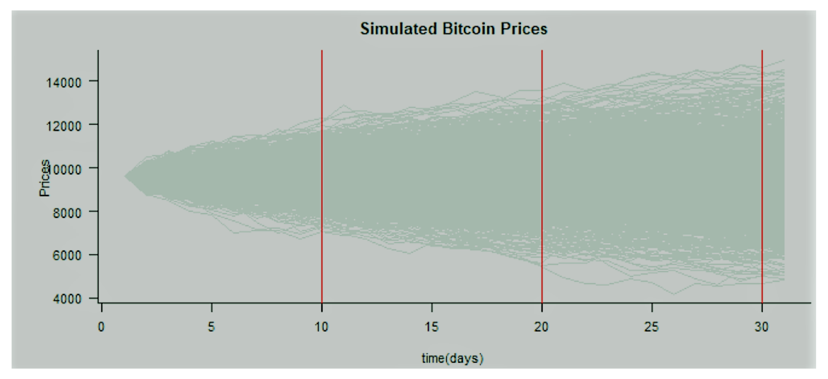
Figure 1. Time-varying parameters.
Forecasting 04 00023 g001
Figure 2. Fitted densities on the log-scale for the series of Bitcoin returns.
Forecasting 04 00023 g002
Figure 3. Bitcoin asset prices.
Forecasting 04 00023 g003
Figure 4. Trajectories of simulated Bitcoin prices.
Forecasting 04 00023 g004
Figure 5. Distribution dynamics of Bitcoin prices at Δ t = 10 ,   20 ,   30 .
Forecasting 04 00023 g005
Table 1. Percentiles of prices.
29 July8 August18 August
Quantiles10 Day20 Day30 Day
25%981295908915
50%10,36010,2839956
75%10,84111,02911,161
90%11,34211,81812,049
95%11,88112,24513,157
99%11,96312,88513,600
mean10,085.6510,085.6610,085.68
skweness−0.0899−0.0891−0.0626
kurtosis1.13900.55110.3755
Publisher’s Note: MDPI stays neutral with regard to jurisdictional claims in published maps and institutional affiliations.

