Forecasting Regional Tourism Demand in Morocco from Traditional and AI-Based Methods to Ensemble Modeling

Abstract

Tourism is one of the main sources of wealth for the Moroccan regions, since, in 2019, it contributed 7.1% to the total GDP. However, it is considered to be one of the sectors most vulnerable to exogenous shocks (political and social stability, currency change, natural disasters, pandemics, etc.). To control this, policymakers tend to use various techniques to forecast tourism demand for making crucial decisions. In this study, we aimed to forecast the number of tourist arrivals to the Marrakech-Safi region using annual data for the period from 1999 to 2018 by using three conventional approaches (ARIMA, AR, and linear regression), and then we compared the results with three artificial intelligence-based techniques (SVR, XGBoost, and LSTM). Then, we developed hybrid models by combining both the conventional and AI-based models, using the technique of ensemble learning. The findings indicated that the hybrid models outperformed both conventional and AI-based techniques. It is clear from the results that using hybrid models can overcome the limitations of each method individually.

1. Introduction

Tourism is considered to be one of the main sources of wealth for the Moroccan economy, since, in 2019, it contributed 7.1% to the total GDP. From economic and social perspectives, the tourism sector enhances the development of local enterprises by creating consequential jobs in local areas, stimulating local demand, as well as being an important source of foreign currency inflow. The development of tourism also tends to have positive benefits which are highlighted through its contributions to the implementation and upgrading of the country’s infrastructures (roads, tourist zones, hotels, hostel, etc.). Despite these advantages, tourism is one of the sectors most sensitive to exogenous shocks (political and social stability, currency change, natural disasters, pandemics, etc.). Various tools have been used by policymakers to sustain the growth of the tourism sector such as marketing, advertising, tourism events, etc. However, scholars tend to use more rigorous methods and multiple key indicators to capture tourism demand, such as tourism demand forecasting, which has become a key instrument for policymakers. Over the past decade, researchers have focused on using traditional techniques such as time series methods, econometric models, qualitative techniques, etc. Recently, researchers have used more rigorous methods such as artificial intelligence-based modeling. To date, only a limited number of researchers have tried to compare the performance of both conventional and AI- based techniques in terms of forecasting accuracy; moreover, none of them have tried to combine them into hybrid models and to assess the results.

The existing literature review reveals that most researchers have adopted the number of tourist arrivals as a proxy for tourism demand [1], for example, a study by [2] used the number of tourist arrivals in Beijing as compared with an internet search index to verify the Granger causality and cointegration relationship. Another study by [3] forecasted tourism demand at 31 intraregional levels of mainland China using international guest arrivals for the period from 1994 to 2007. This work took tourism predicting into a new field of research by exploring intraregional tourism forecasting in China using modern methods (basic structural and time-varying parameter models); the work concluded that forecasting at the intraregional level could be accurate using modern techniques. Another work by [4] used the ten countries with the highest number of arrivals to Hong Kong for the period from 1990 to 2000, using the time series techniques SARIMA and MARIMA; [5] also used six seasonal models including SARIMA modeling.

A study by [6] adopted a broader perspective and used tourism expenditures [6], in which they used multiple econometric models for the period 1969–1999 to generate tourism expenditure forecasts until 2010; the unrestricted VAR was found to have the most accurate results. A study by [7] gave a complete comparison between using the number of arrivals and tourism expenditures as a proxy for tourism demand forecasting; the findings suggested that using tourism expenditures tended to have high levels of inaccuracy explained by the quality of data and related to price changes. In addition, tourism consists of complex subindustry connections making it more difficult to measure.

Conversely, other scholars have used the number of overnight stays [8]. A study by [9] compared tourist arrivals and overnight stays and concluded that adopting tourist arrivals was more accurate than using overnight stays. Alternatively, other researchers have tried to construct more complex proxies such as the tourism composite indicator (TCI), by including macroeconomic and non-economic determinants of tourism demand. In [10,11,12], they reviewed a key list of indicators for both sides of tourism demand and supply. A study by [5] used hotel room demand as an indicator, since it provided the possibility of forecasting using daily-frequency observations.

There is also debate related to appropriate forecasting techniques. The time series methods are the most often used approaches. Such integrated autoregressive moving average (ARIMA) models have become popular in recent years [13,14,15]. Other econometric models have been used, such as the vector autoregressive (VAR) model [6] and vector error correction model (VECM) [16].

A study by [17] reviewed key studies on tourism demand forecasting and addressed different techniques of forecasting that had evolved between 1968 and 2018. A study by [18] identified 155 research articles that had been published and classified into three major groups based on the methodology and techniques adopted, i.e., the econometric approach, time series methods, and AI-based techniques. In addition, [1] reviewed multiple papers related to demand forecasting and found that methods used for forecasting were more diverse than those identified in most studies. [19] attempted to match tourism forecasting in the context of forecasting techniques and data features, and adopted a meta-analysis by examining the link between forecasting model accuracy, data characteristics, and study features. The results revealed that the frequency and period of the data, the main place visited, the country from which visitors arrived, the forecasting techniques, and the proxy used to capture the tourism demand all had substantial impacts on the performance of the forecasted model.

Recently, there has been growing interest in adopting more complex techniques derived from artificial intelligence-based modeling such as machine learning and deep learning frameworks, owing to their accuracy, adaptability, and capability of predicting a nonlinear process. Studies by [20,21,22] suggested that tourism demand was characterized by nonlinear behavior. AI-based modeling provided faster implementation in a real-world challenge with the expansion of data (big data) [23] and data complexity (high data dimension, limited horizon, and volatility), whereas conventional methods failed to deliver accurate results. In other words, unconventional methods outperformed conventional models [21]. Another work by [24] suggested that monitoring tourism demand could be done in real time, which was not possible using conventional models. In the context of Morocco, a work by [25] used four AI-based (long short-term memory, gated recurrent unit, support vector regression, and artificial neural network) techniques to forecast tourist arrivals from 2010 to 2019 using monthly tourist arrival data; the findings suggested that the LSTM and GRU frameworks performed better than the others. [26] used an artificial neural network by examining its capability in the context of COVID-19.

The summary of the literature relating to the proxy adopted to capture tourism demand has shown that the number of tourist arrivals was the most used variable. The review also discussed three main methods, i.e., econometrics, time series, and AI-based techniques used by researchers in the field of tourism demand forecasting.

The main purpose of this study is to forecast tourist arrivals using three different approaches. We start with first-level modeling which is the conventional method based on time series and econometric techniques, and the unconventional method which is drawn from the AI-based techniques capable of dealing with nonlinear behaviors. Finally, in second-level modeling, we combine both conventional and AI-based methods into hybrid models to overcome the limitations of the individual approaches.

The motivation behind this work comes from three perspectives. First, it is related to the context of the study area, where the tourism sector is considered to be one of the main sources of wealth for the Moroccan regions since it contributes to the total GDP, and therefore, forecasting is a crucial technique for policymakers. Second, this is the first research to shed new light on the use of hybrid models for tourism demand forecasting in Morocco at a regional level. Third, the present study fills a gap in the literature related to the debate between conventional methods such as econometric and time series methods and new type of models derived from artificial intelligence techniques with the possibility of hybrid models.

The remainder of this paper is organized as follows: In Section 2, we describe the source for the data and the preprocessing procedures, and then present the metrics used for measuring forecasting accuracy, as well as the theoretical background of all adopted approaches; in Section 3, we analyze the results and findings of the two approaches, and then the hybrid models; in Section 4, we provide a discussion; and finally, in Section 5, we summarize our conclusions and remarks.

2. Materials and Methods

2.1. Data and Preprocessing

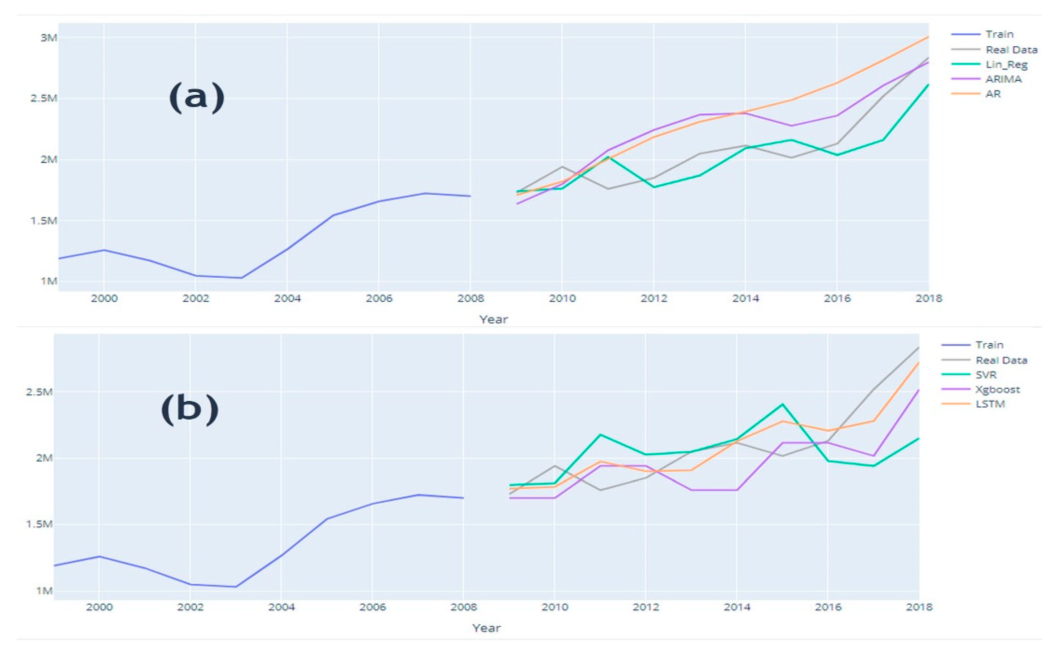
To forecast tourism demand at a regional level, we used the number of tourist arrivals to the Moroccan regions from 1999 to 2018; the data were obtained from the Department of Economic Studies and Financial Forecast in The Minister of Economy and Finance. To validate the efficiency and the performance of the forecasting models, the data were split into two datasets, i.e., the estimating sample (training dataset) and the validation sample (testing dataset).

For more accurate results, the data were divided equally between training and testing (50% as testing data and the rest as training data), that is, data from 1999 to 2008 as training data and data from 2009 to 2018 as testing data. Sometimes data can raise serious issues related to an appropriate splitting scale. Since we had only 19 observations in total, we required the optimal choice for splitting the data. Choosing a small dataset for training could lead to overfitting the model, because the model could adapt excessively by learning all the possible hidden patterns in the data, and therefore, perform poorly in approximation. Conversely, a small testing dataset would likely generate roughly optimistic results.

The conventional and AI-based model approaches both have two different mechanisms of forecasting. It is well known that traditional techniques are limited to capturing only increasing/decreasing linear patterns of data. By using the period 1999–2008 as a training dataset, conventional techniques would succeed in learning the increasing trend (linear pattern) of data. However, using, for example, a random split or different split configuration, would leverage the AI-based model, which is built to handle complex patterns and penalize the traditional methods. In general, we tried to find a middle ground to keep the necessary statistical characteristics of each approach, especially, for the traditional approaches. Technically, we tried different split scenarios; the split selected was used for comparisons.

The data needed min–max scaling between a range of 0 to 1 using Equation (1); some machine learning and deep learning algorithms such as SVR and LSTM rely crucially on feature scaling and can be beneficial in improving forecasting accuracy. Feature scaling was done by using the following formula:

$$z_t=\frac{x_t-x_{min}}{x_{max}-x_{min}}$$

(1)

where $x_{min}$ and $x_{max}$ are, respectively, the minimum and maximum values of the tourist arrivals to each region and $x_t$ is the number of tourists arrivals during year t. If $x_t$ is at the minimum value, the numerator will be 0, then, $z_t$ equals 0. Conversely, if $x_t$ is at the maximum value, the numerator is equal to the denominator, then, $z_t$ equals 1. Alternatively, if $x_t$ is between $x_{min}$ and $x_{max}$, then, $z_t$ is in the range of 0–1.

Regarding the appropriate scaling method, the use of normalization versus standardization has been debated. Using gradient descent as an optimization framework (used by the SVR and LSTM) requires data scaling first. However, standardization scaling is used when dealing with data that contain unwanted extreme outliers; since standardization does not have a bounding interval, it smooths the data. In addition, it is necessary when dealing with features that converge to a normal or Gaussian distribution. Unlike neural network models, SVM, etc., standardization is a mandatory assumption for logistic regression, linear regression algorithms, etc.

Alternatively, normalization is used when the variable/process is behaving in a non-Gaussian distribution/or unknown distribution, which is an assumption that most algorithms do not require (e.g., LSTM, KNN, and SVR). Sometimes data capture shocks, which is a significant factor when the objective of a study is to analyze the impact of these outliers/shocks on the data. In addition, normalization can be used when we have multiple features with a different scale (multivariate analysis). The choice between normalization and standardization is based on each data, study, objective, type of analysis (univariate or multivariate), and type of variable (quantitative, binary, nominal, and categorical), which leads to different results. Taken together, the normalization scaling method tends to suit our case.

2.2. Metrics for Accuracy Measures

Traditionally, conventional models use statistical significance known as the p-value (mostly p < 0.05), but the pretesting process changes the distribution of the estimator parameters. To overcome this issue, researchers use predictive ability with multi-criteria measures, such as the root mean square error (RMSE). The RMSE evaluates the quality of the forecasting by showing the level of deviation between predictions and the actual values using Euclidean distance. The lowest RMSE means that more forecasted data are close to the real data. The RMSE is not robust for scale-invariance, meaning that RMSE is affected by min–max scaling; as a result, this measure is used over scaled datasets. The square is used to sum the percentage errors without attention to sign to compute the RMSE. For the mean absolute percentage error (MAPE), the error is determined as the actual data minus the forecasted data. Because this measure is a percentage, it is easy to understand, i.e., the lower the MAPE value is, the higher the accuracy of the forecast. The mean absolute error (MAE) examines the average of absolute error values of the prediction on all instances of the testing data.

Table 1. The mathematical formula for each metric.

Accuracy Metrics	Formula
RMSE	$\sqrt{\frac{{{\displaystyle \sum }}_{n=1}^N{\left(y_t-{\widehat{y}}_t\right)}^2}{N}}$
MAPE	$\frac{1}{N}{\displaystyle \sum _{n=1}^N}\frac{\left|y_t-{\widehat{y}}_t\right|}{y_t}*100$
MAE	$\frac{{{\displaystyle \sum }}_{n=1}^N\left|y_t-{\widehat{y}}_t\right|}{N}$

Where N is the number of data points (time span), $y_t$ is the actual values, and ${\widehat{y}}_t$ is the forecasted values.

shows the mathematical formula for each metric.

Scaling features should only be applied for traditional techniques. Since we are dealing with a univariate series analysis, scaling is not a necessity when applying traditional techniques. For example, AR or ARIMA methods, indeed, in some cases, can be crucial when the context is a multivariate time series analysis (ARIMAX and VAR). For example, the scale of the predictors has a significant magnitude than the dependent variable, in this case, non-scaling generates estimated coefficients that are large, which amplify the effect of predictions on the dependent variable when the model moves to the forecasting step. While scaling, in the case of small magnitude, will not harm the model.

2.3. Methodology

This study’s primary contribution is to evaluate the performance of various machine learning approaches and compare them to conventional approaches in terms of forecasting accuracy, and then combine the two approaches into hybrid models to overcome the limitations of each approach. On the one hand, for example, ARIMA fails to predict complex patterns [21]; on the other hand, LSTM is a powerful neural network capable of mapping complex patterns. The idea behind a hybrid model is to capture the unique features of a data pattern by each approach, and then combine them into one blended model. For example, if a time series variable has two features, i.e., a linear and nonlinear behavior, using only LSTM captures only nonlinear behavior and the linear behavior is set as an error. Inversely, if we use only the ARIMA model, it captures only the linear part, setting the rest as an error, and if we combine the LSTM and ARIMA the two components linear and nonlinear (nonlinear here represents a model that uses nonlinear parameters) are captured. Researchers have found that hybrid methods that combine nonlinear algorithms and a linear process in time series variables have considerably more significant results [27]; these combined models can be used at the same time to capture both behaviors. The three artificial intelligence-based models used and the three conventional models are summarized below.

2.3.1. Support Vector Regression (SVR)

The SVR attempts to reduce error by finding the hyperplane and minimizing the difference between the forecasted and the observed data. The SVR was found to be more performant in prediction as compared with other approaches such as KNN and elastic net, due to enhanced optimization strategies for a wide range of factors.

The statistical theory behind this method was developed by [28]. Considering the training data as follows:

$$\left\{\left(x_1,y_1\right), \left(x_2,y_2\right), \left(x_2,y_2\right),\dots ,\left(x_N,y_N\right)\right\} \subset R^z\times R,$$

(2)

where $x_t$ is the input vector at time t and $y_t$ is the related tourism demand for every $x_t$. The prediction model is given by the following regression function $f\left(x_t\right)$:

$$f\left(x_t\right)=w^T{x}_t+\beta ,\hspace{1em}\hspace{1em}\hspace{1em}w, x_t\in R^z,\hspace{1em}\hspace{1em}\beta \in R$$

(3)

where $\beta$ is the bias and $w$ is the weight vector. The goal is to obtain an $f\left(x_t\right)$ with highly generalized behavior. For this purpose, the user needs to optimize the model complexity and the training error tolerance. The complexity of the model can be demonstrated by $f\left(x_t\right)$ flatness, meaning having a small weight vector (w). This can be achieved by minimizing the Euclidean norm $\left|\left|w\right|\right|$. To control training error tolerance, we can use the $\epsilon -\mathit{insensitive}$ loss function proposed by Vapnik in 1997. The $\epsilon -\mathit{insensitive}$ loss function ignores errors that are within $\epsilon$ range of the actual value by treating them as equal to zero. The measured distance between the actual value and the $\epsilon$ range can be described using the following expression:

$${\left|\mu \right|}_{\epsilon }=\left\{\begin{array}{c}0 \mathit{if} \left|y-f\left(x\right)\right|\le \epsilon \\ \left|y-f\left(x\right)\right|-\epsilon \mathit{otherwise}\end{array}\right.$$

(4)

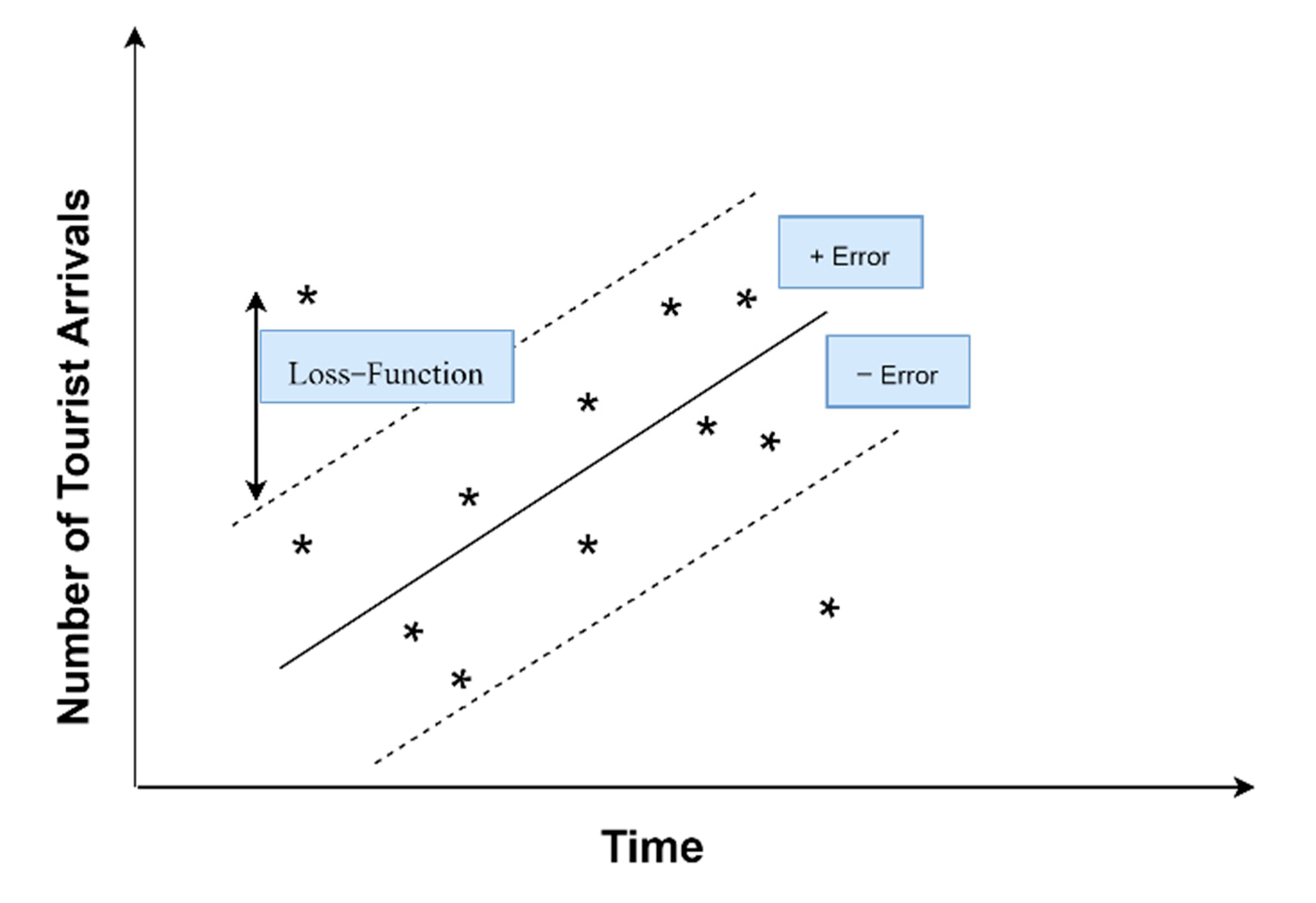
The loss function penalizes the model complexity by penalizing deviations greater than one, which means all training data larger than the $\epsilon -\mathit{insensitive}$ band. As seen graphically in Figure 1, when dealing with a one-dimensional linear regression function using the $\epsilon$ band, all values inside the $\epsilon$ band are equal to zero.

The program that minimizes the error function is as follow:

$$f\left(x\right)={\displaystyle \sum }_{m=1}^M\left({\alpha }_m^{*}-{\alpha }_m\right)x_m^{T}x+\beta ,$$

(5)

$\mathrm{where} {\alpha }_m^{*}$ and ${\alpha }_m$ are defined as Lagrangian multipliers and the training values positioned outside the $\epsilon -\mathit{insensitive}$ tube are referred to as the support vectors. This function can be solved using linear regression in feature space $R^z$ by introducing a kernel function k:

$$f\left(x\right)={\displaystyle \sum }_{m=1}^M\left({\alpha }_m^{*}-{\alpha }_m\right).k\left(x_m^{T}x\right)+\beta ,$$

(6)

Solving $k\left(x_m^{T}x\right)$ relies on using different types of kernels (such as Gaussian kernel, polynomial kernel, and linear kernel), see [28,29] for a full demonstration of the SVR. A full description of the SVR method and its parameters related to tourism forecasting can be seen in [20,30,31,32].

2.3.2. Long Short-Term Memory (LSTM)

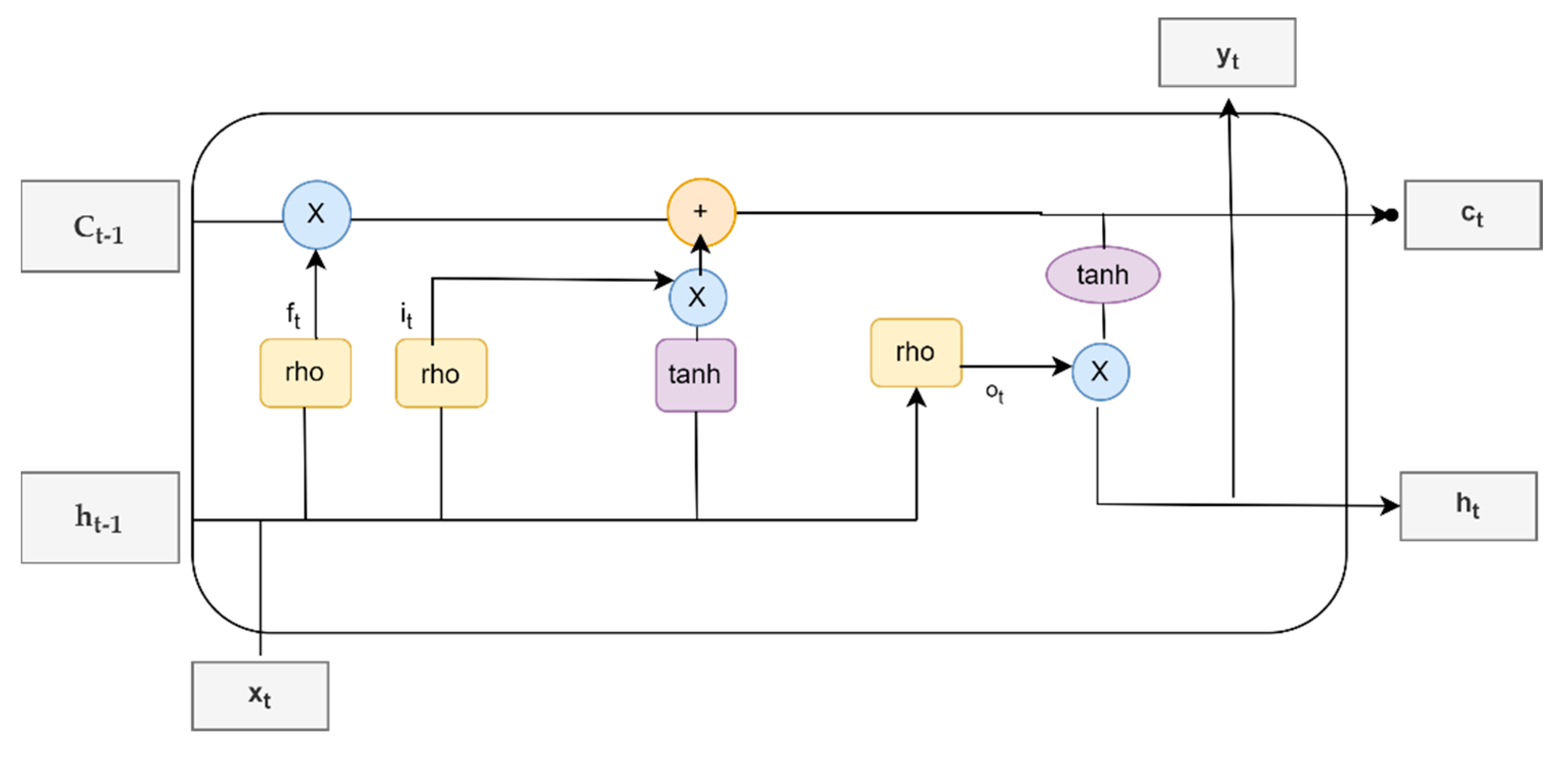
Long short-term memory (LSTM) is the second approach, initially proposed by [33], and is considered to be an advanced recurrent neural network (RNN); LSTM is capable of solving the vanishing/exploding gradient issue that RNN algorithms face. The RNN is unable to recall or remember the long-term independence as a result of a vanishing/exploding gradient (similar to reading a book and not remembering the previous chapters). LSTM models are designed to avoid long-term dependency issues. They can be utilized for classifying and/or predicting using time series data. A typical LSTM architecture contains a memory cell (or the cell state), input gate, forget gate, and an output gate; Figure 2 illustrates the architecture of the LSTM model at a time t as in [25].

The following formulas structure the LSTM model based on two equations:

The equations of the gates:

$$\begin{array}{c}{i}_t=\sigma \left(w_i\left[h_{t-1},x_t\right]+b_i\right)\\ f_t=\sigma \left(w_f\left[h_{t-1},x_t\right]+b_f\right)\\ o_t=\sigma \left(w_o\left[h_{t-1},x_t\right]+b_o\right)\end{array}$$

(7)

where$i_t$ is the input gate;$f_t$ is the forget gate$; o_t$ is the output gate$; \sigma$ is the activation function (logistic sigmoid, tanh, or ReLu)$; w_i, w_f, \mathrm{and} w_o$ are the weight of gates$; h_{t-1}$ is the output of the previous gate at t − 1$; x_t$ is the input at time t$; b_i, b_f, \mathrm{and} b_o$ are the biases of each gate.

The equations of the cell state and the output gates are:

$$\begin{array}{c}{\tilde{c}}_t=\mathit{tanh}\left(w_c\left[h_{t–1},x_t\right]+b_c\right)\\ c_t=f_t*c_{t–1}+i_t*{\tilde{c}}_t\\ h_t=o_t*\mathit{tanh}\left(c^t\right)\end{array}$$

(8)

where $c_t$ is the memory (or the cell state) at time t and ${\tilde{c}}_t$ is a candidate for cell state at time t.

The input gate ($i_t$) determines which data should be added to the cell state. The forget gate ($f_t$) controls whether data from the prior memory should be discarded or preserved. In the end, the output gate ($o_t$) outputs the value. During the processing, it sends the previous hidden state to the next step of the sequence. The neural network’s memory is stored in the hidden state. It stores information about prior data that the network has seen. The first step combines the input and the hidden state forming a vector $x_t$. This $x_t$ has information about the current input and the previous inputs. The $x_t$ passes through the tanh activation function (tanh activation function squishes the data values so that they are always between −1 and 1, to assist in controlling the values that flow through the network); the result or the output is the memory of the network (or the new hidden state). In addition, the logistic sigmoid activation function can be used for squishing data between 0 and 1, and choosing between tanh or sigmoid is based on the data characteristics. According to researchers, tanh and sigmoid functions have been found to have some issues regarding vanishing/exploding gradient. Nowadays, rectified linear activation function (ReLu) activation is widely used and outperforms tanh and sigmoid functions. LSTM is described in detail by [33].

2.3.3. eXtreme Gradient Boosting (XGBoost)

The eXtreme Gradient Boosting (XGBoost) is a supervised learning algorithm proposed by [34]; it is based on the gradient boosting framework’s concepts. It improves the forecasting performance by introducing more regularized model formalization to control overfitting problems using the classification and regression tree (CART).

The XGBoost process can be formalized as follows:

$$\begin{array}{c}\widehat{y_{\mathit{ı}}}={\displaystyle {\displaystyle \sum }_{m=1}^M}{f}_m(x_i),\hspace{1em}{f}_m\in F\\ F=\left\{f\left(x\right)={\omega }_q\left(x\right)\right\}(q={ℝ}^m\to T,\omega \in {ℝ}^T)\end{array}$$

(9)

where $\widehat{y_{\mathit{ı}}}$ is the predicted output, m is the number of CARTs used to illustrate the model, $f_m(x_i)$ is the predicted output in the m-th tree, and F is the space of regression trees. By minimizing the following regularized objective function, it includes the loss function and term of regularization:

$$\left\{\begin{array}{c}L={\displaystyle \sum _{i=1}^n}l\left(y_i,\widehat{y_{\mathit{ı}}}\right)+{\displaystyle \sum _{m=1}^M}\Omega (f_{m)}\\ \Omega (f_{m)}=\gamma T+\frac{1}{2}\beta {\displaystyle \sum _{j=1}^T}{w}_j^2\end{array}\right.$$

(10)

where n is the number of observations, $l$ is the second-order derivative loss function that measures the difference between the real data $y_i$ and the predicted $\widehat{y_{\mathit{ı}}}$, $\Omega (f_{m)}$ is the term of regularization, T is the number of leaves in the tree, $w_j^2$ is the weight of the leaves, and complexity parameter $\gamma$, and $\beta$ to control the tree. The goal of this optimization program is to define the structure of the CART and the weight of each tree, also we cannot optimize in the traditional Euclidean space. However, the program can be solved using an additive manner described in [34].

We choose three conventional techniques, namely ARIMA as the most used time series (TS) model in tourism demand forecasting literature, autoregressive (AR), and univariate linear regression.

2.3.4. Univariate Linear Regression

The linear regression mostly applied to analyze the relationship between a dependent variable $Y_t$ and a dependent variable $x_t$ known as simple linear regression or a set of dependent variables ${\displaystyle \sum }_{i=1}^n{x}_t$ ($i=1,\dots ,n$ is the number of independent variables) which is called multiple linear regression, can be constructed as follows:

$$Y_t={\beta }_0+{\displaystyle \sum }_{i=1}^n{\beta }_i{x}_t+{\epsilon }_t$$

(11)

where ${\beta }_0$ is the constant, ${\beta }_i$ are regression coefficients to estimate, and ${\epsilon }_t$ is the error term in time t. In the case of a simple linear regression, the above equation becomes:

$$Y_t={\beta }_0+{\beta }_1{x}_t+{\epsilon }_t$$

(12)

where $Y_t$ is the target or the output value (the dependent variable) and$x_t$ is the input value. Since we want to use only one variable in the linear regression, Equation (12) becomes:

$$f{\left(\theta ,x\right)}_t={\theta }_0+{\theta }_1{x}_t$$

(13)

In Equation (13), we have only one input feature (tourist arrivals), which is $x_t$; ${\theta }_0$ and ${\theta }_1$ are the regression coefficients; and the univariate linear regression is implemented in scikit-learn library in Python [35]. The purpose of choosing this technique is that it can only capture the linear pattern of the data and the simplicity of its statistical learning makes it much like conventional techniques.

2.3.5. Autoregressive (AR) Model

The autoregressive model is a time series model used to forecast a variable based on its lagged values. The AR model takes the following form:

$$Y_t^{\text{'}}=c+{\displaystyle \sum }_{i=1}^p{\varnothing }_i{Y}_{t-i}^{\text{'}}+{\epsilon }_t$$

(14)

where $Y_t^{\text{'}}$ is the time series values at time t, p is the order of the lag, and $Y_{t-i}^{\text{'}}$ is the lagged values of $Y_t^{\text{'}}$, with ${\epsilon }_t$ as an error term in time t, and c as constant.

2.3.6. Autoregressive Integrated Moving Averages (ARIMA) Model

The autoregressive integrated moving averages (ARIMA) model was first proposed by Box and Jenkins in 1970, after Herman Wold introduced the ARMA model and failed to derive the likelihood function for maximum likelihood (ML) to estimate the parameters. In 1970, Box and Jenkins accomplished this finding, as outlined in the classic book Time Series Analysis. The ARIMA method has three components, using historical data through the autoregressive (AR) part and handling the stochastic factors by using the moving averages (MA) component.

The ARIMA model is expressed as ARIMA (p,d,q), where (p), (d), and (q), respectively, are the order of the AR part, the degree of differentiation, and the order of moving average part.

Mathematically, the ARIMA model can be written as follow:

$${\mathrm{Y}}_{\mathrm{t}}^{\text{'}}=\mathrm{c}+{\varnothing }_1{\mathrm{Y}}_{\mathrm{t}-1}^{\text{'}}+\cdots {\varnothing }_{\mathrm{p}}{\mathrm{Y}}_{\mathrm{t}-\mathrm{p}}^{\text{'}}+{\mathsf{\phi }}_{\mathrm{t}}{\mathsf{\epsilon }}_{\mathrm{t}-1}+\cdots +{\mathsf{\phi }}_{\mathrm{q}}{\mathsf{\epsilon }}_{\mathrm{t}-\mathrm{q}}+{\mathsf{\epsilon }}_{\mathrm{t}}$$

(15)

The ${\mathrm{Y}}_{\mathrm{t}}^{\text{'}}$ is the differenced variable (sometimes variable can be differenced multiple times). On the right side of Equation (15), there is the autoregressive (AR) component as the lagged values of ${\mathrm{Y}}_{\mathrm{t}}^{\text{'}}$, and the moving averages component (MA) as the lagged values of the errors ${\mathsf{\epsilon }}_{\mathrm{t}}$. By using backshift notation, the ARIMA model should be as follows:

$$\left(1-{\varnothing }_1\mathrm{B}-\cdots -{\varnothing }_{\mathrm{p}}{\mathrm{B}}^{\mathrm{p}}\right) {\left(1-\mathrm{B}\right)}^{\mathrm{d}}{\mathrm{Y}}_{\mathrm{t}}=\mathrm{C}+\left(1-{\mathsf{\phi }}_1\mathrm{B}-\cdots -{\mathsf{\phi }}_{\mathrm{q}}{\mathrm{B}}^{\mathrm{q}}\right){\mathsf{\epsilon }}_{\mathrm{t}}$$

(16)

where $\left(1-{\varnothing }_1\mathrm{B}-\cdots -{\varnothing }_{\mathrm{p}}{\mathrm{B}}^{\mathrm{p}}\right)$ is the AR(p) component,${\left(1-\mathrm{B}\right)}^{\mathrm{d}}$ is the order of differentiation, and$\left(1-{\mathsf{\phi }}_1\mathrm{B}-\cdots -{\mathsf{\phi }}_{\mathrm{q}}{\mathrm{B}}^{\mathrm{q}}\right)$ is the moving averages MA(q) part.

The ARIMA model, in some cases, has been found to be more performant than the other complex time series models, such as VAR and VECM.

More recently, researchers have been manually fitting different parameters, as in [13,14,15]. The manual process goes from fitting different models using many orders, and then comparing the features of each model using information criteria: Akaike information criterion (AIC), Bayesian information criterion (BIC), Hannan–Quinn information criterion (HQIC), and corrected Akaike information criterion (CAIC). However, going through this process manually is time-consuming; especially for complex and large datasets, this process minimizes the risk of human error. Python’s prebuilt libraries help to find the optimal parameters such as the order of integration, trend, stationarity, and seasonality in the case of seasonal data for AR/ARIMA models [36], by executing stepwise processing of hyperparameter tuning to identify the optimal parameters (such as p, d, and q for the ARIMA model). Finally, it returns a fitted AR/ARIMA model. The manual selection procedure depends on the autocorrelation function and partial autocorrelation function for ARIMA to determine, respectively, the number of MA terms and the number of AR terms; alternatively, the auto-selection process performs multiple differencing tests such as augmented Dicky–Fuller (ADF), Kwiatkowski–Phillips–Schmidt–Shin (KPSS), or Phillips–Perron (PP) automatically establish the order of differencing. The information criterion is optimized to a minimal value and to the highest for the log-likelihood; this process cycles through different integration orders to obtain the optimal set of parameters. The prebuilt libraries in Python support expending univariate time series, where the parameters can change over time. If the time series present an increasing trend during the observation period, then an increasing tuple should be specified, inversely, a decreasing tuple, when there is a declining trend during the observation time. The model responds automatically to shifting time series patterns and predicts values more accurately. The parameters used for each model are shown in

Table A1. The parameters used for the models.

Model	Parameters
LSTM	optimizer = ‘adam’, loss = ‘mean_squared_error’, batch_size = 1, epochs = 300
XGBoost	objective = ‘reg:squarederror’, n_estimators = 1000
SVR	Kernel = “linear”, C = 1, gamma = “auto”, epsilon = 0.1
ARIMA	order = ([1,2,3,4],2,0), trend = ‘n’
AR	lags = [1,2,3],trend = “n”
Ensemble learning	algo = LassoCV(positive = True)

.

2.3.7. Robust Forecasting Using Ensemble Learning

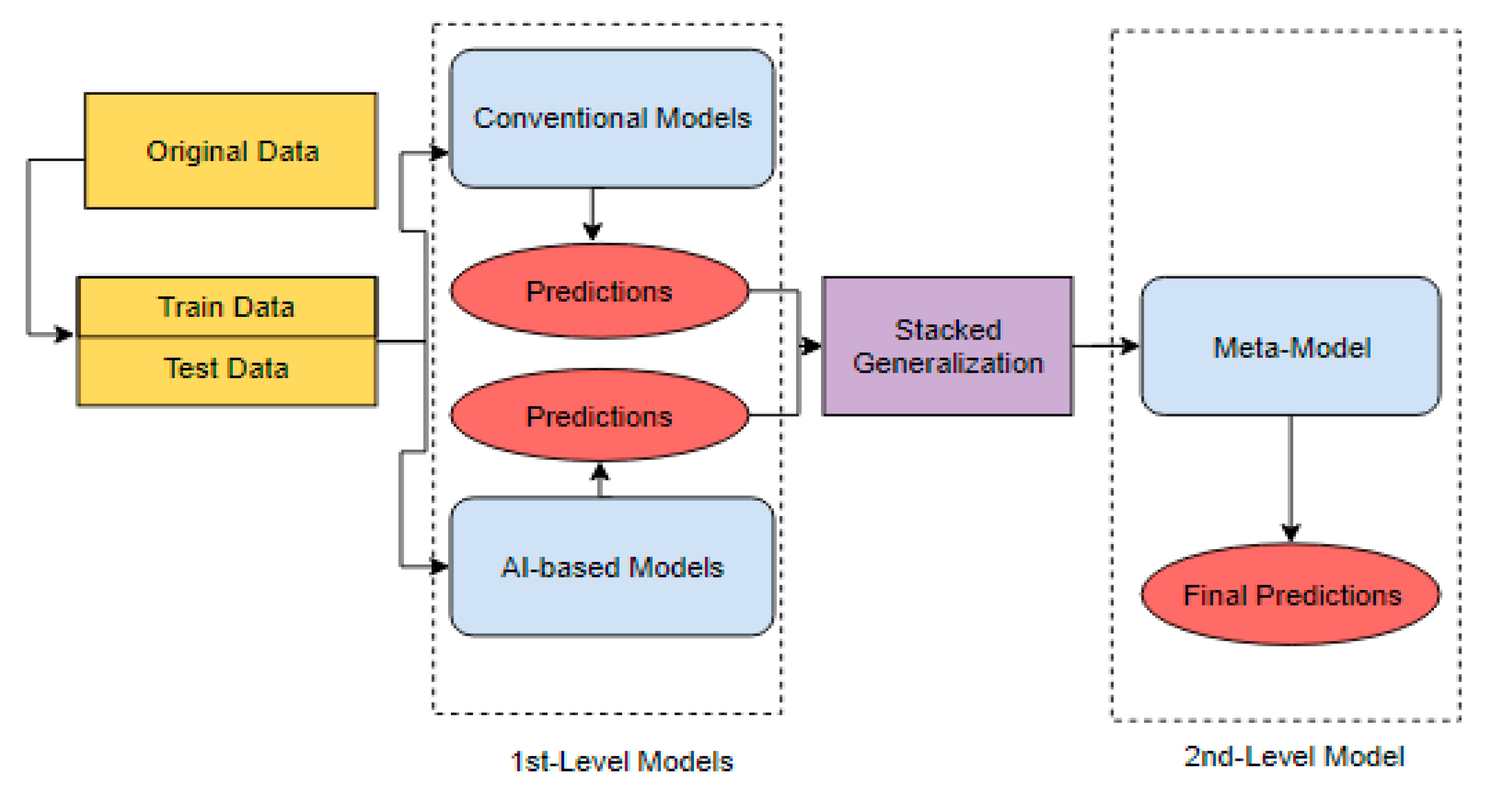
Robust forecasting can be done by merging two models or more, for example, combining an ARIMA model and LSTM results in a hybrid model. The technique of combining models, known as ensemble learning or ensemble modeling, consists of blending output predictions from different machine learning algorithms. The major advantage of using ensemble learning is that it can take many forms such as bagging (or bootstrap aggregating), boosting, adaptive boosting (AdaBoost), mixture of experts, stacked generalization, etc.

Since each method solely tends to capture different patterns and each method has its own biases and prediction errors, by combining methods, they can cancel each other’s errors, leading to robust predictions. Hybrid models tend to have robust results [21] and are less overfitted. In this paper, we adopt the stacked generalization methodology, because of its flexibility, such as combining deep learning algorithms with machine learning models and artificial neural network models, and others; also setting multiple hyperparameters on the same hybrid model. The stacked generalization technique was first introduced by [37], this ensemble learning technique was used for minimizing the generalization error rate from one model or more than one model (known as first-level model or base models), by deducing the biases of errors concerning a given learning dataset. As shown in Figure 3, we combine first-level model predictions, by taking one model from conventional techniques and one model from AI-based models; hence, this blending sets out a second-level model (also called a meta-model or blending model) which uses the first-level predictions as training to determine how to blend and assign weights to the final predictions. The meta-model is constrained by using LASSO which stands for least absolute shrinkage and selection operator, developed by Tibshirani in 1996. This algorithm is based on a linear regression model that can let the meta-model learn from non-negative coefficients only, and can avoid the collinearity among the base models (first-level predictions).

Using the LASSO-learning function solves the question of which approach should have the highest weight; LASSO regression ensures that ensemble learning assigns a zero or a positive weight to each approach automatically [35]. The LASSO learns which model is the most accurate and assigns 1. Alternatively, a somewhat accurate model is assigned less than 1, and in some cases, if the first-level model appears to be inaccurate it assigns zero to each base model.

3. Results

The number of tourist arrivals to the Moroccan regions is forecasted only for the Marrakech-Safi region for the period 1999–2018, which is considered to be the most visited region in Morocco and can be considered to be a benchmark for the other regions. Forecasting was done using three conventional techniques (namely autoregressive model, ARIMA, and linear regression) and three AI-based models (namely LSTM, SVR, and XGBoost). Finally, combined modeling is based on the two approaches to overcome the limitations of each approach individually. The prediction accuracy of all models was assessed using three different measures: MAE, RMSE, and MAPE (see

Table 2. Forecasting accuracy of the Marrakech-Safi region for all the models.

	Model	MAE	RMSE	MAPE (%)
Conventional Models	ARIMA	214,158.6175	241,754.5817	10.841468
	AR	269,820.0817	303,538.1567	12.99072
	Lin_Reg	154,085.0944	185,612.9382	7.195004
AI-Based Models	XGBoost	211,996.5625	259,479.9072	9.692244
	SVR	262,583.4312	347,404.7287	11.876725
	LSTM	130,324.425	154,514.3182	6.272656

). Some of the models are implemented using Python from [38]. The parameters used for each model are shown in Table A1 in Appendix A.

3.1. Forecasting Results and Findings of the First-Level Models

By using the period 1999–2008 as a training set, the conventional techniques successfully capture an increasing trend observed in the real data (see Figure 4a), since the statistical mechanisms of the adopted traditional techniques learn from the historical data. For example, the number of tourist arrivals in 2008 depends on the number of tourist arrivals in 2007 which is captured by AR(1), leading to mapping an increasing number of tourist arrivals. The evolution of the ARIMA and AR trends are close and have similar behaviors even if the two lines show some high forecasted values; however, the trend is the same as the real data. The linear regression shows significant results in terms of matching the real data graphically. Table 2 provides the accuracy metrics of the three conventional methods; the linear regression model shows superior results with the lowest MAPE (7.19%), RMSE (185,612.9382), and the MAE (154,085.0944).

Interestingly, it appears from Table 2 that the linear regression outperformed the ARIMA and AR techniques. Taken together with Figure 4a and Table 2, the results suggest that there is a linear pattern in the number of tourist arrivals captured by the three traditional techniques.

3.2. Results and Findings of the Second-Level Models

However, Figure 4b graphically compares the forecasting results for the Marrakech-Safi region of the three AI-based methods with the real data. The three models behave differently, as each method has its mechanism. The forecasted patterns may be explained by the fact that the algorithms try to capture the nonlinear process using their own set of learning and mapping capabilities. The unconventional methods exhibit a volatile behavior which signifies the ability to map the smooth nonlinearity process; nevertheless, previous knowledge about the regional tourism sector indicates that an increasing trend exists, while the SVR model illustrates an increasing-decreasing pattern which does not agree with the actual data.

From Table 2 we can examine the performance of the unconventional models. The LTSM model shows superior results with the lowest MAPE (6.27%), RMSE (154,514.3182), the MAE (130,324.425) values, followed by XGBoost, and then SVR. Finally, the results of the LSTM model were superior to the other models, with the minimum metrics criteria, indicating the smallest deviations between the forecasted value and the real data. Generally, according to the results of the first-level models, the LSTM technique outperformed all the AI-based models, as found by [25].

Another window to compare between both approaches, as shown in

Table 3. Running time required for implementing each approach.

Approach	Model	Time to Implement Each Strategy
Traditional techniques	AR	17,949 μs
	ARIMA	687,695 μs
	Linear Regression	1005 μs
AI-based models	LSTM	11 s
	SVR	14 s
	XGBoost	676,290 μs
Ensemble learning	LSTM_AR	46,406 μs
	LSTM_Linear	989,630 μs
	LSTM_ARIMA	474,366 μs
	XGBoost_ARIMA	178,725 μs

Note: All models were executed using Colab, the free-hosted Jupyter notebook service offered by Google Research. In addition, the reported ensemble learning time does not include the required time for the base models.

, is the total time required to implement each model. Conventional techniques are known for their statistical simplicity, and therefore require less time and computational capability. However, the results may change when dealing with a high-dimensional dataset, where the standard techniques behave poorly and sometimes fail. Alternatively, the AI-based models require time for learning and mapping all the possible patterns existing in the data, using complex equations that take more computational sources. Here, only the traditional and the AI-based models are compared. Introducing the hybrid model is not wise, due to the fact that the time required to implement ensemble learning relies on the time it takes the base model to forecast, meaning we need to take into consideration the time required to implement base models.

However, the results for LSTM_ARIMA were anticipated since this model combines ARIMA as the most used traditional technique [13,14,20] and LSTM an advanced neural network algorithm.

Finally, the hybrid models illustrated in

Table 4. Forecasting accuracy of the Marrakech-Safi region for the hybrid models.

Model	MAE	RMSE	MAPE (%)
LSTM_AR	128,462.6305	149,117.1278	6.127097
LSTM_LINEAR	133,713.4925	169,222.7763	6.538672
LSTM_ARIMA	165,065.2356	211,778.9905	7.548610
XGBOOST_ARIMA	203,038.5896	219,668.8450	9.800446

and Figure 5 outperformed the individual models, except for the XGBoost_ARIMA, this hybrid model shows an increase in the accuracy metrics, where the MAPE of the XGBoost model goes from 9.69% individually to 9.80% when combined with the ARIMA model (the same increase observed for the rest of accuracy measures). Consequently, the hybrid models sometime may fail to improve accuracy, due to inadequacies between the different mechanisms of each base model.

Regarding second-level modeling Figure 6, the results for LSTM_AR indicated it was the most significant ensemble learning model, where adding a model capable of mapping linear pattern and another model capable of mapping nonlinear behavior improved the accuracy, as found by [20,27]. After combining both approaches using ensemble learning, the model learns to switch between the two patterns, i.e., to the linear pattern when the coefficient related to the traditional techniques is superior to the one for the unconventional model, and to the nonlinear pattern when the inverse happens, thus, leading to better mapping of the real data, and increasing the accuracy significantly.

4. Discussion

According to our findings and those of previous studies, ensemble learning is promising since it takes advantage of every single model that is included, which leads to minimizing forecasting errors and outperforming individual standard models [39]. Among the previous works that used hybrid models, none of them found that conventional techniques outperformed the strategy of hybrid models [39,40], which is considered to be groundbreaking for the technique of ensemble learning. Hybrid models became a new trend in tourism forecasting between 2008 and 2017, as reported [39], whereas, prior to 2008, only four studies had examined the use of combining models in the tourism literature.

However, this technique requires more attention regarding which base model should we include, as some data can be affected by both the linear and nonlinear processes, which need a set of combined techniques capable of dealing with both behaviors [20,27].

Sometimes, including a time series technique in a hybrid model can be crucial, especially when a periodic pattern is present in a dataset, such as seasonality, trends, and cyclicity, where the traditional time series techniques have gained renowned respect [5,10,11]. However, time series combined, for example, with a neural network framework will significantly improve accuracy [20], or add features capable of mapping those repeated cycles despite having a short dataset [22].

Some researchers have used advanced techniques to increase the number of observations in the case of having an insufficient dataset, which have alleviated issues related to a lack of sufficient data. For example, using a rolling window [5], where the purpose of this strategy was to create “new” (the word new here adds many questions when dealing with traditional techniques such as time series) observations based on a previously observed sample. However, adopting those strategies in the case of a time series model (as a base model) will certainly change the statistical characteristics (trend, stationarity, etc.) of the created subsamples and the rolling windows, leading to inadequacy through the subsamples. Its like creating multiple variables with no primary processing steps (unit root test, autocorrelation, normality test, etc.) used in time series analysis inside the original variable. Since some subsamples are stationery and others are not, it is a matter of chance, which is unacceptable in statistical inference.

Introducing traditional techniques among the hybrid components may be challenging, especially in the preprocessing step of the data, as those methods need more accurate specifications to be implemented for forecasting, such as ensuring the stationarity, autocorrelation, increasing/decreasing trend, linearity, standard asymptotic, and the normal distribution, which are essential when dealing with time series assumptions. In addition, AI-based techniques also require attention when choosing the optimal parameters [41].

Which model should have the highest weight, is another question with respect to using hybridization techniques Some methods (LASSO, SWITCH, etc.) may have the answer. For example, the SWITCH algorithm tests the difference between hybrid models that include different components. The weight will be equal when the difference is statistically insignificant, otherwise, the best base model should be used individually if the difference is significant [39]. Adopting the LASSO function, as we did, ensures that ensemble learning will assign a zero or a positive weight to each approach automatically. The LASSO learns which model is the most accurate and assigns 1. Alternatively, a somewhat accurate model is assigned less than 1, and in some cases, if the first-level model appears to be inaccurate it assigns zero to penalize the error occurred by this base model.

None of the reviewed studies appeared to have discussed the total time required to implement each model, which is considered to be crucial when forecasting in real time as in [24] or dealing with high-dimensional data. According to our findings, conventional techniques tend to perform well in this competition, compelled by less processing complexity. In contrast, the AI-based models tend to take substantially more time due to their complexity when learning all the possible patterns, which requires more computational resources. The situation may be the inverse when dealing with high-dimensional data, where the conventional techniques failed to handle the task.

Tourism demand forecasting is a key instrument for policymakers. It has attracted the attention of researchers since the tourism industry plays a crucial role in the economic development of some regions such as the Marrakech-Safi region. Developing more accurate results helps governments, policymakers, investors, and tourism management to prepare the necessary infrastructure (roads, tourist zones, hotels, hostels, etc.) capable of serving the number of tourists by developing anticipated strategies. The pursuit for absolute accuracy in tourism demand forecasting has led researchers to use different approaches. Time series, econometric models, and AI-based techniques continue to attract scholars; however, a new type of model appears to be superior to all the previous approaches, taking advantage of all techniques in a complex hybrid model.

It is beyond the scope of this study to capture the impact of COVID-19 due to the restricted regional data availability after 2018, which limits the scope of analysis. Despite the success demonstrated by the three approaches, a significant limitation is the small sample size, which limits the conventional methods from finding a trend and expressive relationship. Using high-frequency data (monthly, seasonal, or weekly) could surely overcome this obstacle, and this issue should be anticipated and addressed in future research. Some studies have used non-official data such as using online reviews and internet big data from a search engine [2,23], or business sentiment surveys [24]; these new approaches of gathering data could open a window to limitations related to data availability.

5. Conclusions

In this study, we set out to forecast the number of tourist arrivals to the Marrakech-Safi region using three AI-based models versus three other conventional techniques, we evaluate their forecasting accuracy, and then we combine the two approaches in hybrid models to overcome the limitations of each technique. The findings showed that the AR model had the most significant results among the conventional techniques, while the LSTM outperformed all the AI-based models, which showed significant output values and successfully mapped the pattern of the real data. The second major finding was that the hybrid model that combined LSTM and AR models was consistently more accurate as compared with the other combined techniques and the base models.

Taken together, these results suggest that forecasting tourist arrivals cannot be done using a conventional or AI-based model solely. However, for results with high significance, researchers should combine different techniques to overcome the limitation of each technique individually, since each approach captures a unique feature of the data. The contribution of this study has been to show the differences between the techniques of conventional models (such as time series and econometric-based models) as compared with artificial intelligence-based models, as having two different methodologies, since they have different principles and mechanisms.

Further research could explore other possible hybrid models such as combining more than two models in one ensemble learning technique with different weighting algorithms Other studies could assess the difference between different techniques of ensemble learning when using mixed-frequency data which has been shown to be the new trend in tourism demand forecasting. Generally, more research is needed in explainable AI-based modeling.