Study on Lateral Vibration of Tail Coach for High-Speed Train under Unsteady Aerodynamic Loads

Abstract

As the speed of high-speed trains increases, the vehicle’s lateral stability steadily deteriorates. There have been observations of abnormal vibrations in the tail car, particularly on certain sections of the railway line. This study built a high-speed train aerodynamic simulation model for a three-car consist, and a multibody dynamics simulation model for an eight-car consist based on numerical simulations of train aerodynamics and multibody dynamics. It investigated both steady and unsteady aerodynamic loads, flow field characteristics, and the dynamic performance of vehicles under varied aerodynamic loads at 400 km/h. The results indicate that the aerodynamic loads generated during high-speed train operation exhibit highly unsteady characteristics. Steady aerodynamic loads have a relatively minor impact on the vehicle’s dynamic performance, whereas unsteady loads exert a more significant influence. Under unsteady aerodynamic forces, the tail car experiences severe lateral vibrations. The lateral stability index, displacement, velocity, and acceleration of the tail car under unsteady conditions were measured at 2.26, 7.54 mm, and 0.53 m/s², respectively. These values represent increases of over 17.71%, 148.84%, and 111.24%, respectively, compared to the steady loads. Large oscillation amplitudes result in more significant lateral displacements and accelerations of the vehicle. This phenomenon is a crucial factor contributing to the “tail swing” effect observed in high-speed trains. This study emphasizes the importance of considering unsteady aerodynamic effects in assessing the lateral stability of high-speed trains and highlights the significance of mitigating the adverse impacts of such dynamic responses, particularly in the tail car.

1. Introduction

The continuous increase in railway operating speeds has posed severe obstacles to railroad safety. Poor lateral stability during train operation on specific rail lines has grown increasingly common in recent years. In some cases, the train’s rear end’s stability deteriorates dramatically in comparison to the front end, resulting in pronounced lateral oscillations that significantly reduce passenger and crew comfort. Once such periodic lateral oscillations appear at the rear end, they are difficult to self-attenuate, even after leaving specific track sections. High-speed trains (HST), characterized by their high length-to-diameter ratio and operation in proximity to the ground, experience complex turbulent vortex structures in the near-wake region. In contrast to the front end of the train, the oscillatory aerodynamic forces generated by these vortex structures lead to reduced lateral stability at the rear of the train. Consequently, recognizing the impact of aerodynamic loads on the abnormal lateral oscillations of the tail car of HST has become a critical technological challenge that must be overcome to enhance railway speeds.

As operational speeds have increased, the coupling effects between HSTs and the surrounding air environment have become increasingly severe [1,2]. In recent years, researchers have principally focused on HST fluid–structure coupling dynamics [3], with an emphasis on examining the impact of vortex structures in the surrounding flow field on the dynamic performance of these trains. Tian’s research [4] discovered that vortices are formed predominantly by complicated surface discontinuities and regions of considerable curvature. Vortex distributions were discovered to be localized in the bogies and inside the wake region. The presence of vortices beneath the train has a substantial impact on the train’s lateral stability during the hunting of HST. Hemida et al.’s observation [5] that enormous vortex formations shed in the HST‘s wake zone during crosswinds significantly affect the unsteady aerodynamic forces. The lateral vibrations of the vehicle are exacerbated because the aerodynamic forces produced by vortex shedding in the wake region oscillate at a frequency that closely matches the train’s lateral vibration frequency. For ICE2-type trains, they also performed Strouhal number analysis. Experiments revealed that the complicated airflow patterns in tunnel environments had a considerable influence on the lateral translation and yawing motion of the train’s rear. Diedrichs et al. [6] conducted a comparative aerodynamic analysis within tunnels for the ICE2 and 300 series Shinkansen trains, concluding that the deterioration of train stability is caused by low-frequency unstable airflow prompted by minimal clearances between the train and tunnel walls. Jeon et al. [7] observed substantial swaying of the HEMU-430X train during operation and demonstrated that efficient vibration reduction could be obtained by modifying the placements of anti-hunting dampers and increasing damping. Gao et al. [8] developed a 42-degree-of-freedom vehicle dynamics model, indicating that the vertical vibrations of the car body greatly increase when unstable aerodynamic loads and random track excitations are coupled. Yao et al. [9] constructed a lateral vehicle dynamics model and used it in conjunction with a semi-empirical nonlinear vortex-induced vibration model to simulate fluid–structure coupling lateral dynamics during vortex-induced vibrations. They investigated relevant mitigating techniques, such as modifications in vehicle suspension characteristics, to understand the process of rear-end lateral vibrations caused by vortex shedding-induced body vortex vibrations. Liu et al. [10,11] explored carbody vibrations under various conditions using physical experiments and simulations. According to their results, train body vibrations mostly manifest as low-frequency rolling and lateral swaying under the influence of aerodynamic forces, with the tail vortex also experiencing vertical oscillations due to train body rolling. Ji et al. [12] proposed a fluid–structure coupling method and validated its effectiveness through line tests and dynamic model experiments. Building upon this, they further investigated the fluid–structure coupling characteristics of HSTs passing through tunnels, demonstrating that the HST’s tail swinging upon exiting the tunnel results from the combined effects of aerodynamics and track irregularity. Wang et al. [13] identified different ranges of aerodynamic coefficients capable of inducing low-frequency oscillatory behavior under varying aerodynamic loads and concluded that the low-frequency swinging of the tail car is primarily induced by aerodynamic lift. Dumitriu et al. [14] employed numerical simulations to investigate the impact of a rigid-flexible coupled car body model on the vertical vibration characteristics of the car body. Li et al. [15] explored the impact of a vortex generator installed on the tail car on the aerodynamic characteristics of the train. This study showed that the vortex generator in front of the separation point triggered flow separation and destroyed the balance between separation and longitudinal vortex. It effectively reduces the intensity of the separation vortex at the rear of the train, thereby reducing the aerodynamic resistance and aerodynamic lift of the tail car.

The central focus of current research lies in unraveling the dynamic mechanisms responsible for the lateral swaying observed in HSTs. Many prior investigations in the realm of fluid–structure coupling have made use of constant aerodynamic load coefficients or simplistic vortex-induced models, which serve as stand-ins for the genuine aerodynamic features of trains. Unfortunately, these approaches fall short of accurately representing the intricate, unsteady, three-dimensional airflow patterns surrounding trains. In light of this, there is an immediate and compelling need to delve into the enigmatic lateral oscillations of HSTs when exposed to unsteady aerodynamic forces. This research endeavors to comprehend the intricate interplay between oscillatory aerodynamic loads and the hunting motion of the vehicle. The overarching objective is to effectively curtail lateral vibration accelerations at the rear of the train, prevent train resonance instability, bolster overall train stability, and enhance operational safety. Consequently, a comprehensive grasp of the fundamental principles underpinning train tail-swing motion becomes paramount for realizing future speed enhancements in HSTs while ensuring secure train operations.

2. Computational Model

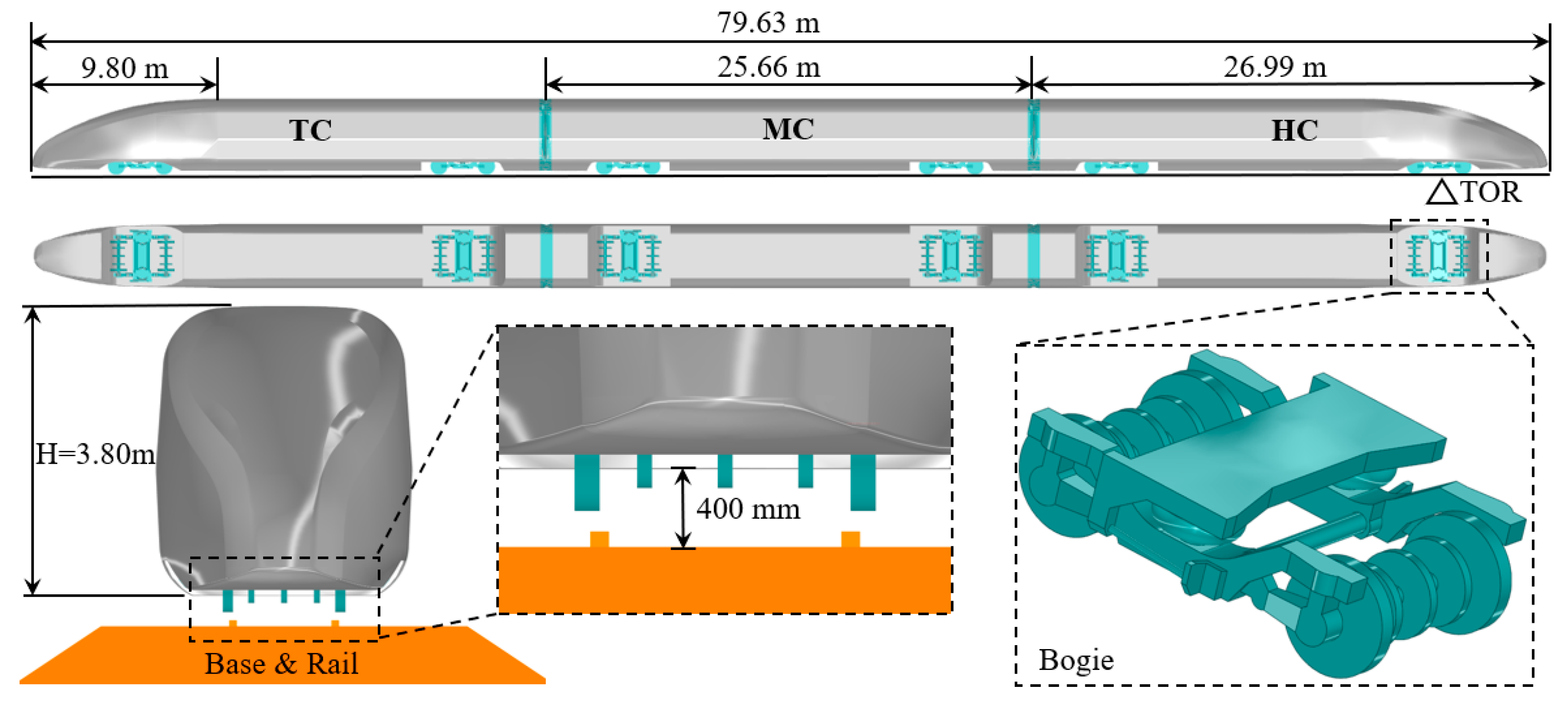
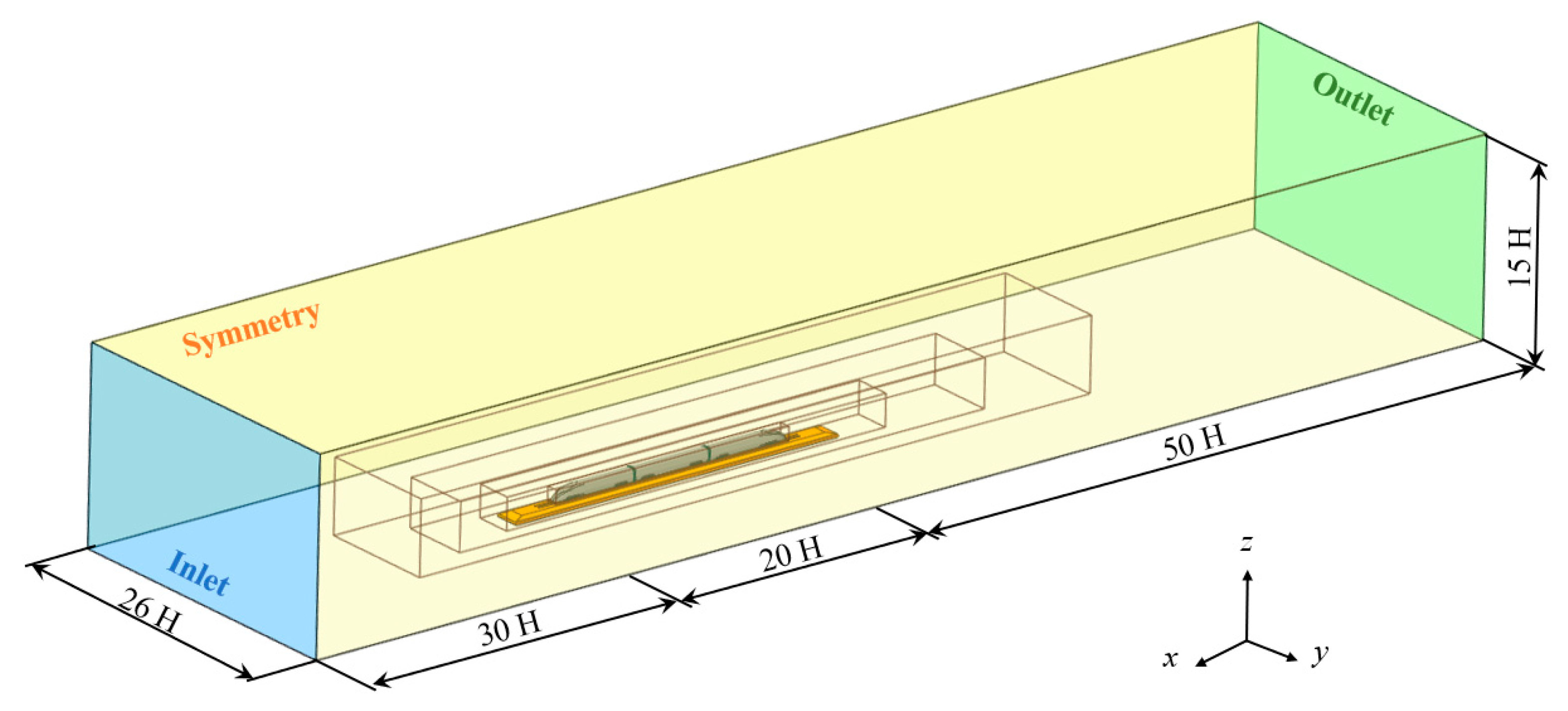
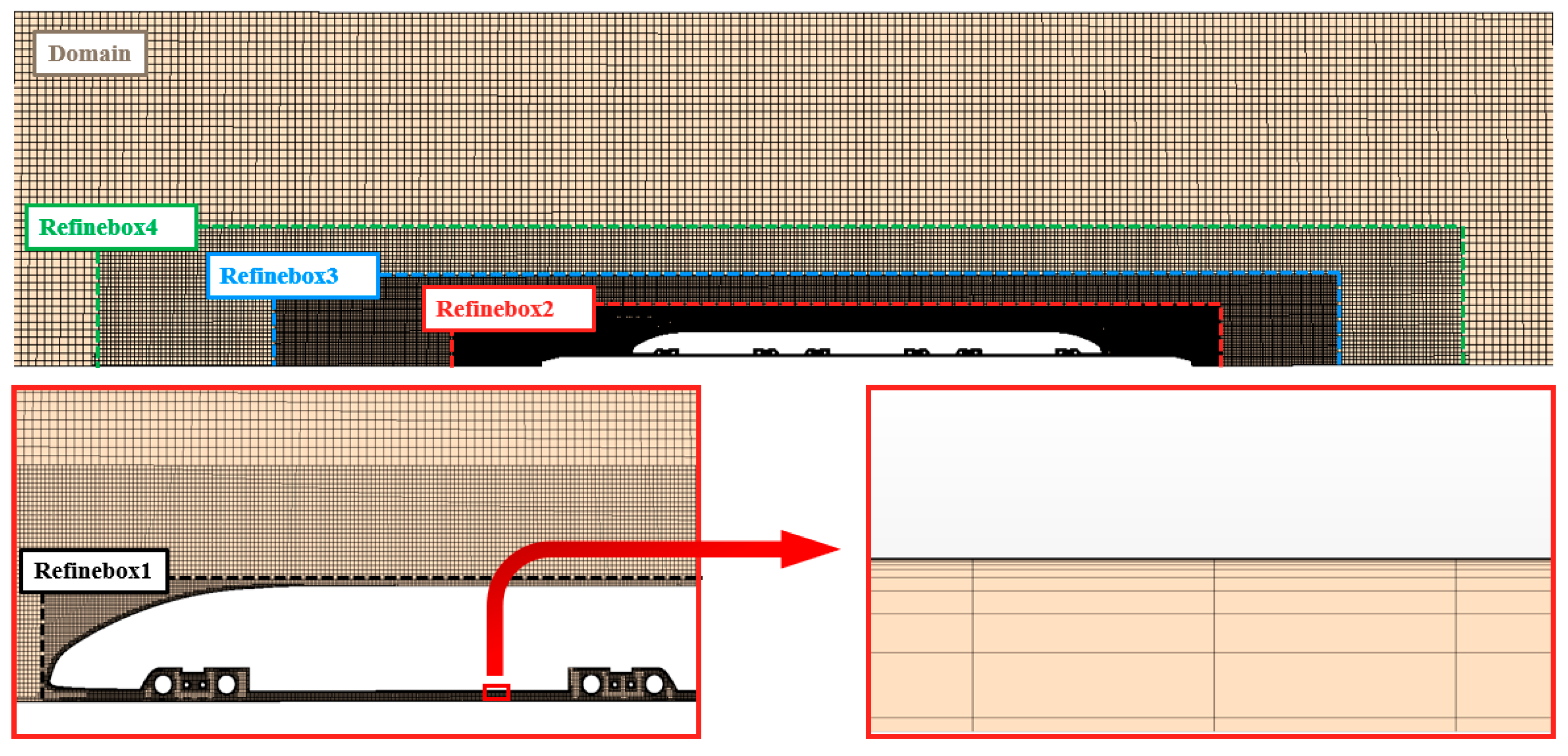
2.1. Aerodynamic Model of three-Car Formation Train

This study focuses on the Chinese domestically developed HST CR400BF. The aerodynamic numerical simulation is conducted using a three-car formation consisting of a head car (HC), an intermediate car (MC), and a tail car (TC). The HC and TC each have a length of 26.99 m, with a streamlined portion of 9.80 m, while the intermediate car has a length of 25.66 m. The entire length of the three-car train is 79.63 m, and the characteristic height (H) is 3.80 m. Each vehicle’s chassis includes two bogies that provide support and guidance. The bottoms of the bogies form the base and rail. The lowest point on the train body is raised 400.00 mm above the top surface of the base, which is identical to the height utilized in wind tunnel tests and related experiments. Some complicated surface structures and pantographs have been eliminated for clarity. The car-end connection adopts a full-cover windshield (Figure 1). depicts the geometric model for the HST’s aerodynamic numerical simulation.

Figure 2 illustrates the outer flow field region for the aerodynamic numerical simulation of the HST. Apart from the base and rail established at the bottom of the computational domain, the remaining boundaries consist of the inlet, outlet, ground, lateral sides, and top. The computational domain is defined based on the train’s characteristic height H, extending 100 H in the x-direction, 26 H in the y-direction, and 15 H in the z-direction. The Inlet boundary at the front of the HC is set to free-flow conditions with a Mach number of 0.3268, corresponding to an inlet velocity of 400 km/h. The Outlet boundary is identical to the Inlet boundary with a combined velocity U_inflow of (−111.11 m/s, 0, 0), where the negative sign indicates that the airflow is in the opposite direction to the train’s motion. The computational domain’s lateral sides and top are defined as symmetric boundaries, whereas the ground, base, and rail are classified as moving walls to eliminate ground effects [16]. The magnitude and direction of the velocity are the same as the input velocity. To ensure a smooth transition of grid cells and improve grid quality and simulation accuracy, four layers of refinement zones are placed around the train, preventing divergence of results caused by abrupt changes in grid scale during the computation process.

The flow field around the train can be thought of as a three-dimensional compressible viscous turbulent flow field with a Mach number of 0.3268 and a Reynolds number of around 2.8 × 10⁷. It is critical for simulating turbulent flow while performing numerical computations of the HST’s external flow field. The turbulence modeling approach employed is the widely adopted improved delayed detached eddy simulation (IDDES) method [17]. As a hybrid turbulence model, IDDES combines the advantages of Reynolds-Averaged Navier–Stokes simulations (RANS) and Large Eddy Simulation (LES) methods, allowing for more accurate modeling of the train’s boundary layer and the capture of large-scale turbulent flow in the far wake. This approach is well-suited for the investigation of the train’s aerodynamic characteristics in this study. For the RANS portion of the simulation, the k-ω Shear Stress Transport (SST) two-equation model is selected as the turbulence model. Compared to the standard k-ω model, the SST k-ω model achieves more accurate solutions for the boundary layer flow on the train’s surface by introducing additional terms related to transverse dissipation and considering the transport process of turbulent shear stress [18]. The convective terms in the momentum equations are discretized using a mixed numerical approach. In the LES portion, a mixed finite-volume scheme based on the Blended Compact Difference Scheme (BCDS) is utilized, whereas in the RANS region, a second-order upwind method is used [19]. The time integration is carried out using a second-order implicit scheme, with a physical time step of approximately $\Delta t=0.015T_{\mathit{inflow}}=5\times {10}^{-4}$ where $T_{\mathit{inflow}}{=\mathrm{H}/\mathrm{U}}_{\mathit{inflow}}$, and the number of inner iterations is fixed at 20. All simulations begin with converged and stable RANS computations as initial inputs and then transition to unsteady IDDES numerical simulations. The overall physical simulation duration for unsteady computations and monitoring is set to 5.0 s, corresponding to 10⁴ time steps.

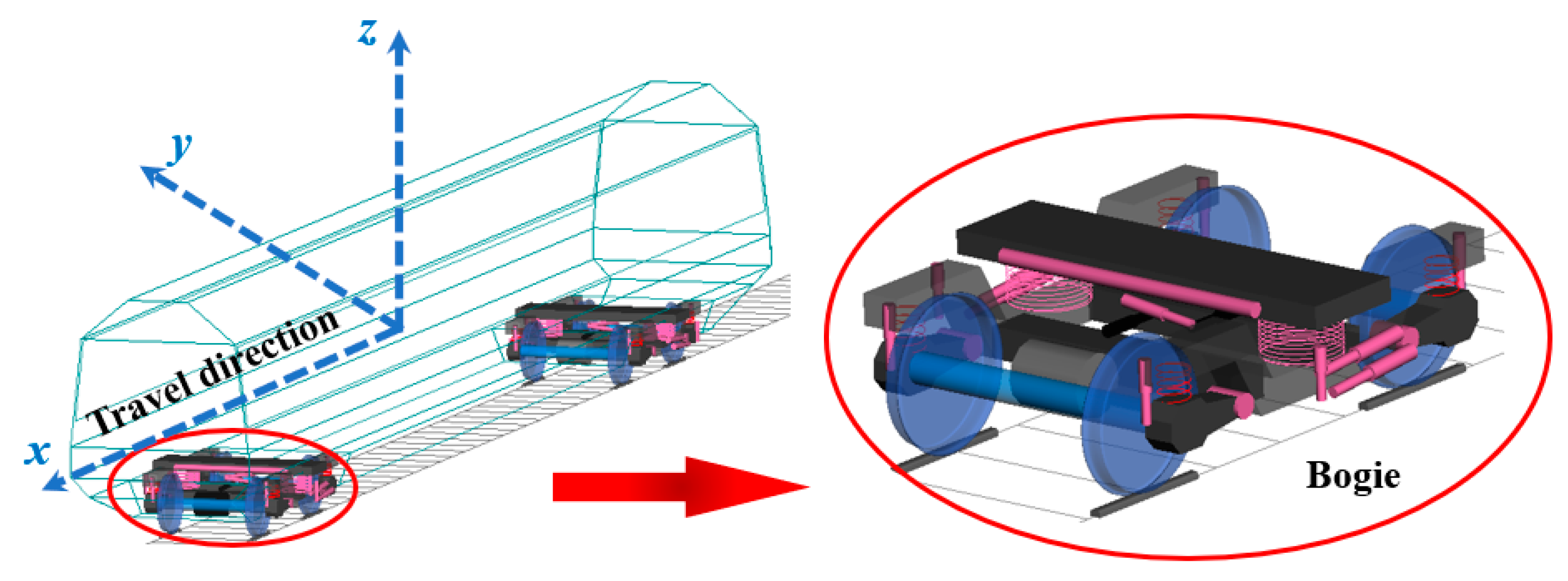
2.2. Multibody Dynamics Model of Eight-Car Train

The multibody dynamics model of an eight-car formation of the HST consists of four motor cars and four trailer cars. Each vehicle is composed of one car body, two bogies, eight suspension arm axle boxes, and four wheelsets. Additionally, each motor bogie includes an extra traction motor. Elastic deformations of the rigidly coupled system formed with these components are neglected. Among the mentioned components, only the suspension arms apply rotational joints around the x-axis, representing only the pitching degree of freedom. The carbody and bogies account for six degrees of freedom in total, considering longitudinal, lateral, vertical, roll, pitch, and yaw directions. The vehicle system is simplified into a multi-rigid-body system with 50 degrees of freedom. The train formation follows the pattern of “motor-trailer-motor-trailer-trailer-motor-trailer-motor”. Connections between each railcar are established using force elements to simulate simplified coupler forces and inter-car windshield forces. The overall HST model has a total of 400 degrees of freedom. For the suspension system components, a first-stage suspension system is established between the wheelsets and bogies, while a second-stage suspension system is established between the bogies and carbody. The motor car model also includes a traction motor suspension system. All dampers in the model are simulated using series-connected spring-damper units, and input functions are configured to simulate the nonlinear characteristics of damper damping and lateral stoppage forces. The final dynamic model of the train is depicted in Figure 3, a loaded measured track spectrum from a specific location in China to account for track irregularities, including lateral and vertical excitations.

3. Simulation Method Validation

In this study, numerical simulations were conducted using simulation software STAR-CCM+ and Simpack for both train aerodynamics and multibody dynamics. To validate the influence of grid scale on simulation results, three sets of grids, labeled Coarse, Medium, and Fine, were generated with base sizes of 1500 mm, 1300 mm, and 1100 mm, respectively, for grid independence testing. The number of grids for each set was 22.55 million, 28.19 million, and 33.53 million, respectively, resulting in a grid number increase of up to 48.7%. The surface of the train was divided into a 13-layer boundary layer with a first-layer thickness of 0.015 mm, a growth rate of 1.6, and surface y+ values around 1.5. To eliminate scaling effects during the validation process, the aerodynamic model was scaled to 1:8, the same as the wind tunnel test. The computation domain for the train’s external flow field and boundary layer grids are illustrated in Figure 4.

The results for pressure coefficient C_p, aerodynamic drag coefficient C_d, and aerodynamic lift coefficient C_l were compared using dimensionless coefficients among the three different grid quantities. These coefficients are as follows.

$$C_{\mathrm{p}}=\frac{P}{0.5\rho U_{inflow}{}^2}$$

(1)

$$C_{\mathrm{d}}=\frac{F_{\mathrm{d}}}{0.5\rho U_{inflow}{}^2\mathrm{S}}$$

(2)

$$C_{\mathrm{l}}=\frac{F_{\mathrm{l}}}{0.5\rho U_{inflow}{}^2\mathrm{S}}$$

(3)

In the equations provided: P represents pressure, ρ stands for air density, S denotes the maximum cross-sectional area of the train, taken as 0.187 m², F_d represents aerodynamic drag, and F_l represents aerodynamic lift, U_inflow represents the inlet velocity, which is equal to 111.11 m/s.

From

Table 1. Comparison of aerodynamic drag coefficients C_d and aerodynamic lift force coefficients C_l of HC, MC, and TC predicted using different grids.

Force	Grids	HC	Error	MC	Error	TC	Error	Total	Error
Drag	Coarse	0.112	1.75%	0.070	0.00%	0.113	0.88%	0.295	1.01%
	Medium	0.114	—	0.070	—	0.114	—	0.298	—
	Fine	0.113	0.88%	0.069	1.43%	0.113	0.88%	0.295	1.01%
Lift	Coarse	−0.026	3.70%	0.000	0.00%	0.090	3.45%	—	—
	Medium	−0.027	—	0.000	—	0.087	—	—	—
	Fine	−0.028	3.70%	0.000	0.00%	0.088	1.15%	—	—

, it can be observed that the predicted drag and lift coefficients for the three grid sets are close. Taking the Medium grid as the baseline, the drag coefficient for the HC is 1.8% higher than the Coarse grid and has an error of less than 0.1% for the Fine grid. The drag coefficient for the TC has an error of less than 0.1% for all grid sets. The lift coefficient for the HC is 3.7% higher for the Coarse grid and 3.7% lower for the Fine grid compared to the Medium grid. The lift coefficient for the TC is 3.45% lower for the Coarse grid and 1.15% lower for the Fine grid compared to the Medium grid. It can be seen that as the number of grid cells increases, the errors in the train’s aerodynamic coefficients gradually decrease, and the results converge.

The analysis indicates that the IDDES algorithm used in this study can reliably and accurately simulate the aerodynamic characteristics of HSTs. Since computational accuracy is positively correlated with the number of grid cells, it is important to avoid excessive grid cell counts that can lead to longer solution times and reduced computational efficiency while ensuring accuracy. For subsequent modeling, this study selects the grid corresponding to the Medium grid with a base size of 1300 mm.

4. Results and Discussion

When HSTs operate at a high-speed level, the surrounding flow field becomes complex, and the unsteady characteristics of aerodynamic forces and torque in terms of both magnitude and frequency become significant; this causes considerable changes in the train’s dynamic performance. The research on abnormal lateral vibrations of the HST’s TC under aerodynamic loads is conducted based on two aspects: the steady/unsteady characteristics of HSTs and the dynamic performance of the train. First, numerical simulations are carried out to investigate the aerodynamic characteristics of each HST vehicle under steady and unsteady conditions at a speed level of 400 km/h. The aerodynamic loads of three vehicles in the unsteady flow field and the surrounding flow field structure are compared. Second, this study focuses on the stability indicators of the TC under different aerodynamic loads. Factors leading to abnormal lateral vibrations of the TC are analyzed based on the amplitude and frequency of the aerodynamic loads.

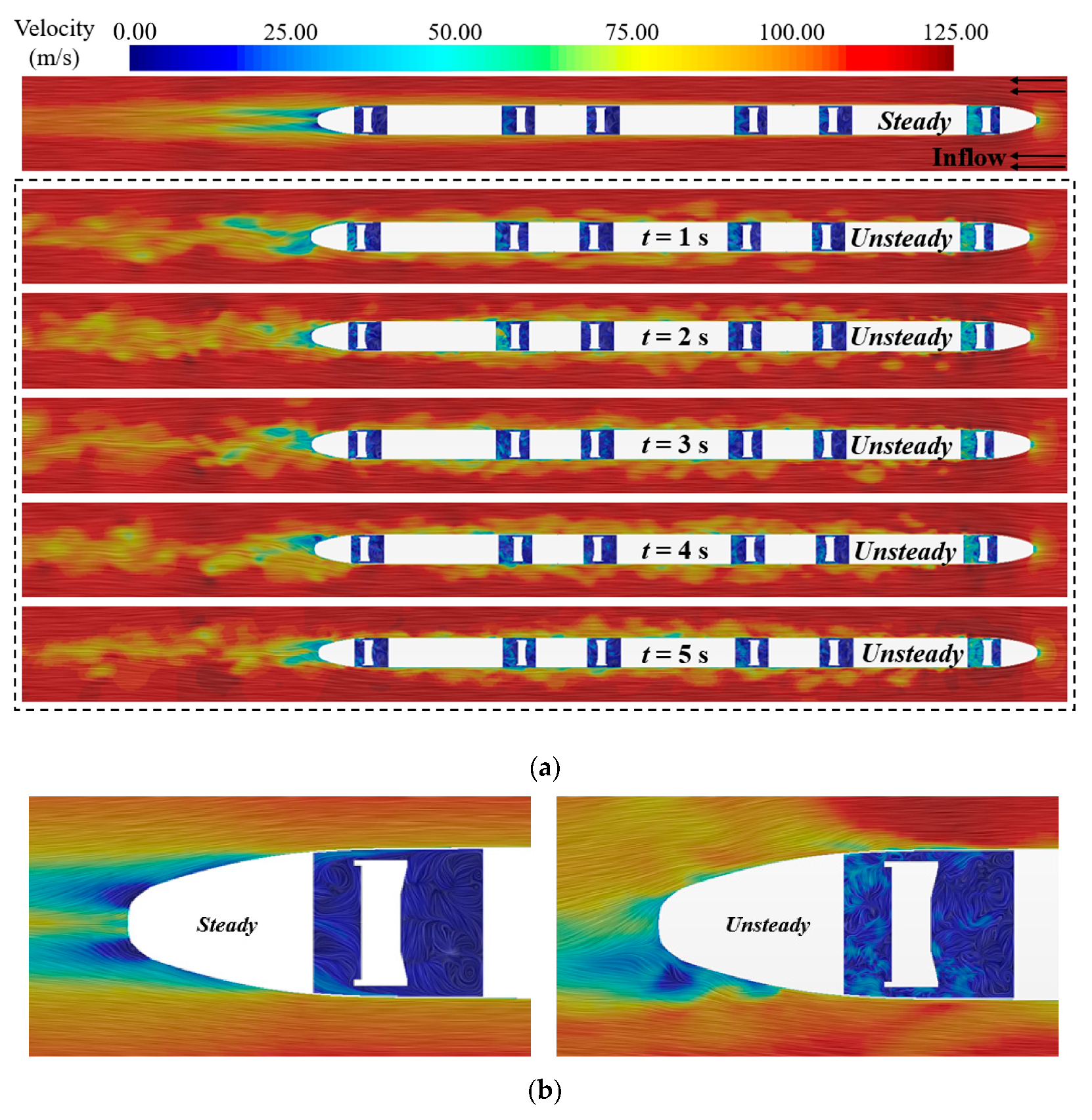
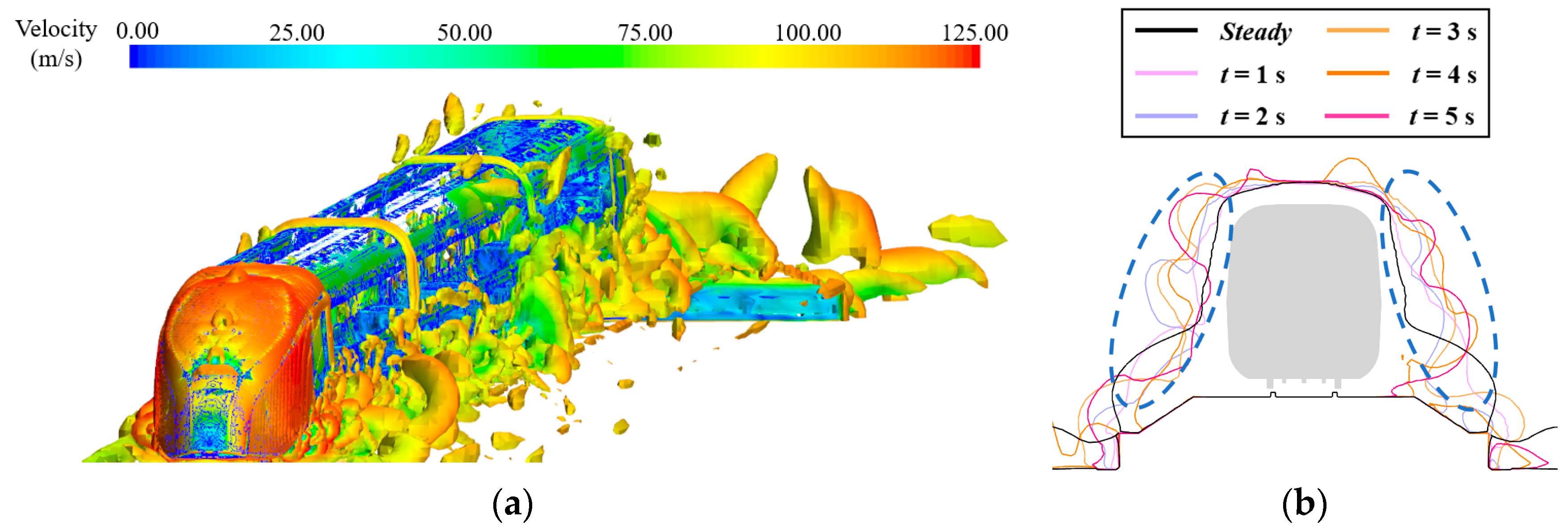
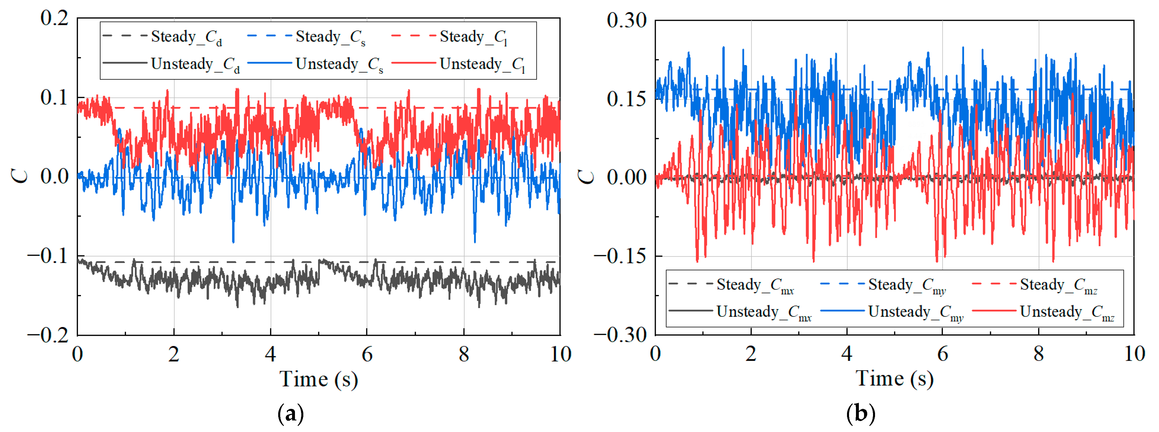
4.1. Research on Steady and Unsteady Aerodynamic Characteristics of HST

In previous research, scholars often used steady-state computational methods based on Computational Fluid Dynamics (CFD) to simulate the steady aerodynamic characteristics of train external flow fields and then load to solve the dynamic response of the train. This approach is relatively cost-effective and less time-consuming but cannot accurately capture the unsteady characteristics of the flow field around the train. In this study, both steady-state (RANS) and unsteady (IDDES) numerical simulations were performed to investigate the aerodynamic characteristics of the train. Figure 5a displays the velocity contours of the horizontal cross-section flow field of the train. In the steady flow field, there is no significant formation or shedding of vortices on either side of the train, except for the development of a symmetrical vortex street in the wake region. In contrast, in the unsteady flow field, the vortices around the train exhibit oscillatory shedding at different physical time points, demonstrating highly noticeable unsteady characteristics in the vortex structures. Similarly, Figure 5b shows a series of smaller-scale vortices around the bogie region in the unsteady case, indicating more complex vortex structures compared to the steady case.

HSTs generate multiple vortex-shedding structures on both lateral sides of the train at higher speeds, as seen in Figure 6a. Use the Q-criterion to identify the vortex cores on both sides of the train, where Q is 500 s⁻². These changes in vortex structures result in variations in the velocity boundary layer of the flow field. Figure 6b depicts a vertical cross-section at the TC’s center of gravity, which is −24.87 m, perpendicular to the x-axis. The changes in velocity boundary layers over time are primarily observed in the regions enclosed by the blue dashed lines on both sides of the vehicle. According to the Bernoulli principle, variations in flow velocity directly lead to fluctuations in surface pressure at the corresponding locations.

The pressure changes on the train’s surface during vortex shedding result in oscillations of the aerodynamic load amplitudes and frequencies. The comparison of aerodynamic loads for the TC is shown in Figure 7a,b. The solid lines represent the unsteady loads of time history, while the dashed lines represent the steady ones. It can be observed that the steady solution’s aerodynamic loads are roughly equivalent to the average of the unsteady ones. However, the steady loads cannot accurately capture the amplitude and frequency variations over time, especially for the aerodynamic side force, rolling moment, and yawing moment, where the steady results are approximately 0; this overlooks the characteristic of these loads oscillating around zero in real-world scenarios. It is evident that the oscillations in the aerodynamic side force coefficient of the TC are much more significant, resulting in larger oscillations in the coefficients of the rolling moment and yawing moment associated with it. Among these, the oscillations in the yawing moment coefficient induce attitude changes similar to the train’s lateral hunting motion, making it susceptible to lateral coupling resonance of the train. Furthermore, The aerodynamic lift coefficient of the TC remains consistently positive, indicating an upward force perpendicular to the ground. This upward lift force also contributes to the deterioration of the TC’s stability.

The influence of the direction of these loads on lateral stability is also visible in the train’s dynamic performance. The oscillation load amplitudes and frequencies can easily couple with the suspension modes of the vehicle, leading to increased lateral amplitude and acceleration of the car body during the hunting motion process due to the coupling effect of aerodynamic forces.

Table 2. RMS value of unsteady aerodynamic forces of the HST.

	Cd	Cs	Cl	Cmx	Cmy	Cmz
TC	0.129	0.024	0.062	0.004	0.136	0.062

shows the RMS values of unsteady aerodynamic loads for each vehicle of the HST.

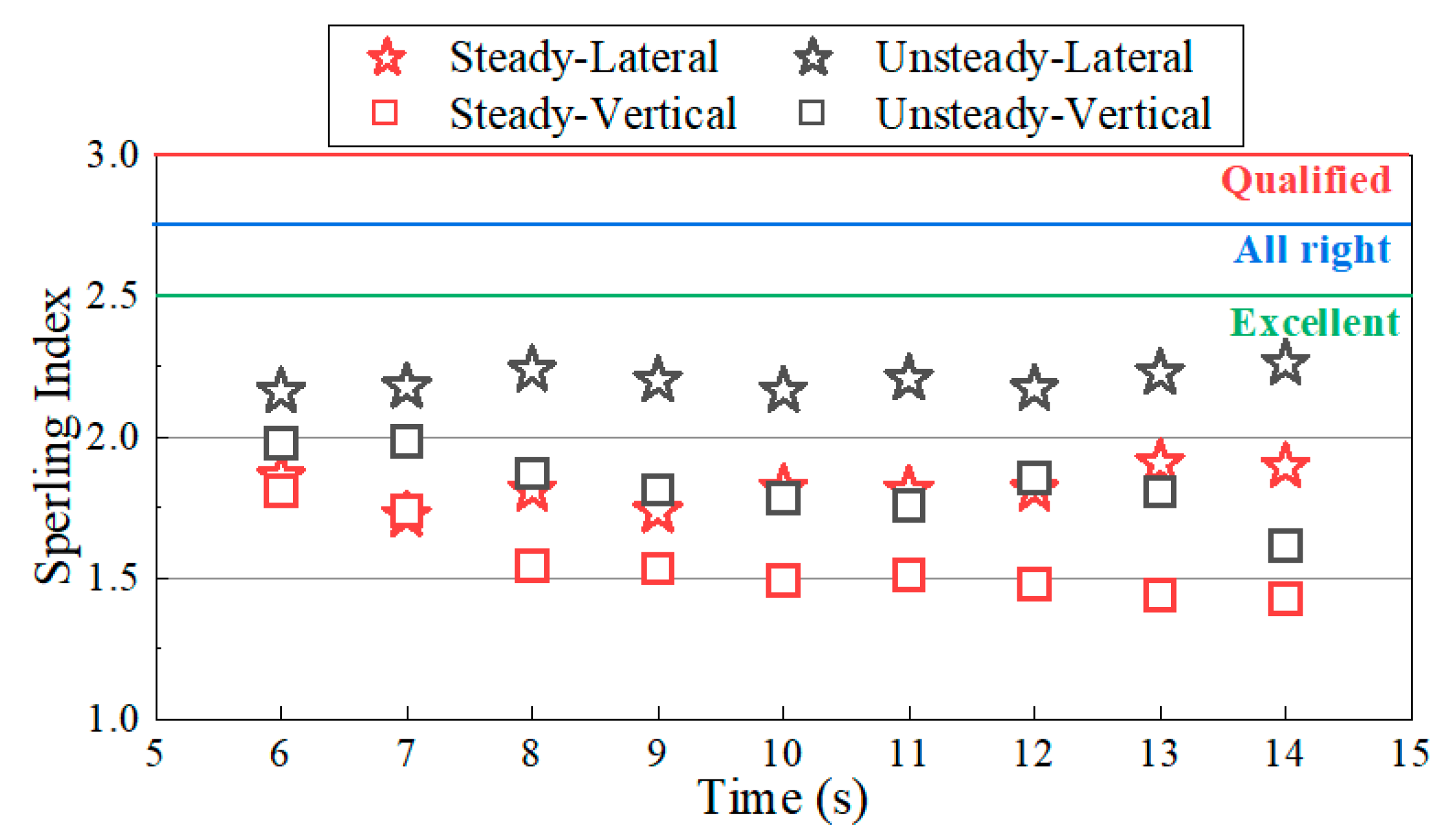
4.2. Research on the Stability of the Trailing Car under Aerodynamics Influences

The lateral abnormal vibrations of the TC often occur in long-formations of the HST, especially when the wheel tread equivalent conicity is low, resulting in relatively intense swaying. In Section 4.2, the dynamic response simulation used an eight-car formation train model with S1002CN wheel profiles, and the equivalent conicity matched with the CN60 rail profile is 0.184. The lateral stiffness of the car body windshield is 0.1 MN/m.

Figure 8 shows a scatter plot of the stability indicators of the train without considering aerodynamic effects, with one datum processed every 2 s. Overall, the stability of each vehicle is satisfactory, and the maximum values of the lateral and vertical stability indicators do not exceed 2.0, fully matching the criteria for excellent stability indicators [20]; this suggests that, without considering the aerodynamic load, although the lateral stability index is slightly larger than the vertical stability, the overall stability is still far less than the limit value, and the stability index meets the requirements.

Both steady and unsteady aerodynamic loads from the CFD simulations in Section 4.1 were applied to the multibody dynamics model to simulate the train’s dynamic response. Figure 9 depicts the Sperling index for various aerodynamic loads. When the steady aerodynamic loads are applied, the impact on the stability of the TC is minor. The index values and time change trends almost coincide with those without considering the aerodynamic load. The maximum lateral Sperling value remains the same as the train without aerodynamics at 1.92, and the maximum vertical Sperling value is 1.81 for the TC, all of which meet the excellent rating criteria. However, upon the application of unsteady aerodynamic loads, considerable variations in the train’s dynamic response emerge. The lateral stability of the TC exhibits varying degrees of deterioration. The lateral Sperling index of TC completely exceeds the 2.0 threshold, with the peak reaching the highest value at 2.26; this represents a substantial 17.71% increase compared to the train without aerodynamics configuration and the scenario involving steady aerodynamic loads, approaching the boundary of the rating criteria. The maximum vertical Sperling value is 1.91 for the TC, reflecting a relatively smaller increase when compared to the train without aerodynamics. As a result, unsteady aerodynamic loads have a considerable impact on lateral stability in real flow conditions, notably the car body of the TC. In contrast, the impact on vertical stability is noticeably less evident.

The lateral accelerations and phase portraits of the TC at the carbody rear end were extracted. In Figure 10a, the amplitude and trend under the conditions of no aerodynamic load and steady aerodynamic load are almost the same. When steady loads are applied, the lateral acceleration of the car body exhibits minimal deviation from the train without aerodynamic configuration. In this case, the lateral vibrations primarily result from the irregularities of the track, indicating that steady loads have a negligible impact. When unsteady aerodynamic loads are imposed, the lateral acceleration in the rear end of the car body experiences a significant increase. The maximum amplitudes of lateral accelerations at the rear end of the TC corresponding to the above three cases are 0.245 m/s², 0.249 m/s², and 0.526 m/s², respectively; this shows that when unsteady aerodynamic loads are applied, the lateral acceleration oscillation amplitude and frequency of the rear end of the TC body increase significantly. It is more than 111.24% higher than the train without aerodynamic force. This severe vibration seriously affects the comfort of passengers and the safety of the journey.

Figure 10b shows the phase portraits of the rear end of the car body with different aerodynamic influences. In three cases, the maximum amplitudes of the lateral displacement are 3.03 mm, 3.04 mm, and 7.54 mm, respectively. Steady aerodynamic loads have a minor impact on the lateral displacement plots, suggesting that even steady loads cannot induce low-frequency lateral instability in the TC. In contrast, unsteady loads result in a sharp increase in the lateral displacement plots, signifying the presence of low-frequency oscillations. These oscillations cause the maximum lateral displacement of the TC to reach 7.54 mm, representing an increase of 148.84%; this implies that the larger amplitudes of aerodynamic lift, lateral force, roll moment, and yaw moment on the TC contribute to a substantial deterioration in its dynamic performance due to low-frequency lateral oscillations. Consequently, influenced by the varying aerodynamic load amplitudes of each vehicle, the entire train formation exhibits a “tail swing” phenomenon that compromises operational stability and passenger comfort.

In summary, the lateral dynamic performance of the TC is significantly worse under the influence of unsteady aerodynamic loads compared to steady ones. Furthermore, the amplitude and frequency of unsteady aerodynamic loads have a considerable impact on dynamic responses. Specifically, the TC suffers more adverse effects due to the larger amplitude and lower dominant frequency of oscillating loads. These characteristics result in deteriorated lateral stability indicators.

5. Conclusions

Through numerical simulations of a three-car consisting of the HST model traveling at a speed of 400 km/h and an eight-car consisting of the multibody dynamics model, this study investigated the influence of steady and unsteady aerodynamic loads on the abnormal lateral vibrations of the HST’s TC. The following conclusions were drawn:

(1)

Aerodynamic loads generated during HST operation exhibit strong, unsteady characteristics. The oscillation amplitude and frequency of aerodynamic loads directly impact the vehicle’s dynamic performance. It was discovered that using only steady aerodynamic loads cannot accurately capture the three-dimensional flow field around the train;

(2)

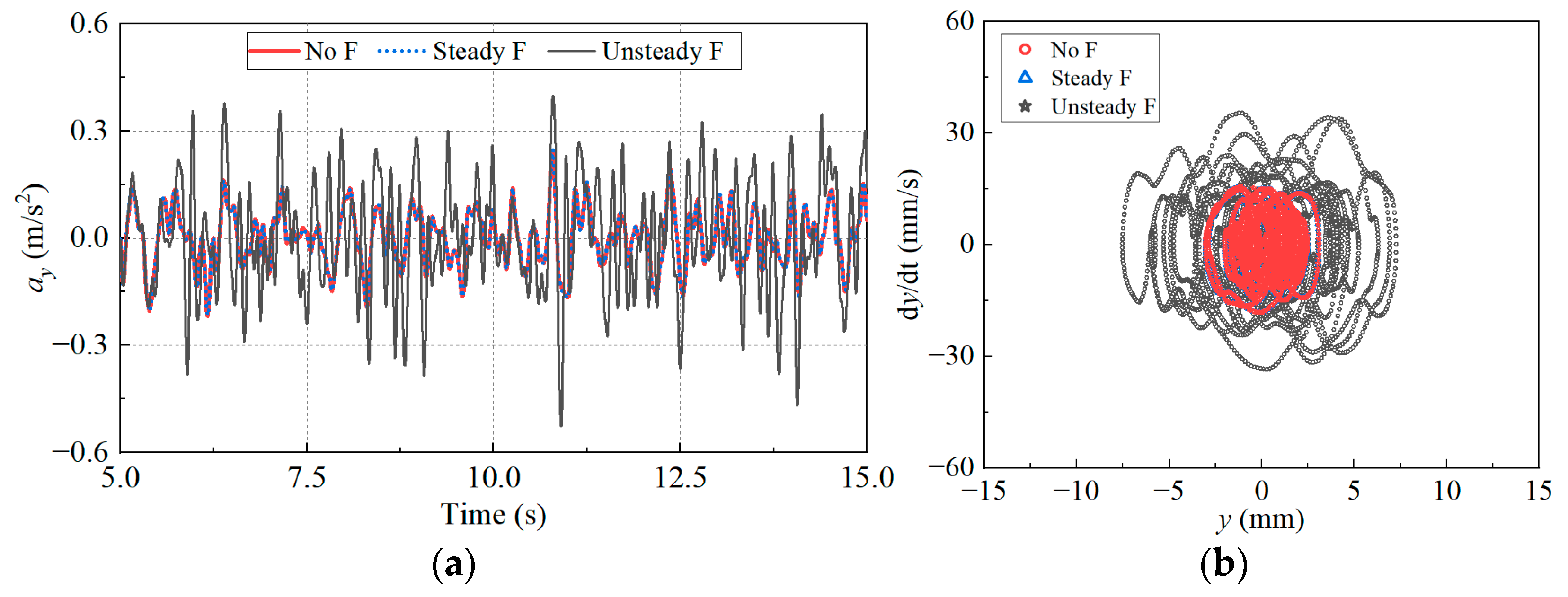
The effect of steady aerodynamic loads on the dynamic performance of the train is minimal. Under unsteady conditions, however, the lateral Sperling index and the accelerations in the rear end of the TC considerably rise in value; this causes severe excessive lateral vibrations in the TC, particularly in cases of low wheel-rail equivalent conicity, and may result in a lateral stability index that exceeds the prescribed level;

(3)

The oscillation amplitude and frequency of unsteady aerodynamic loads are the direct cause of the deterioration of vehicle lateral stability. The larger the amplitude, the greater the lateral vibration displacement and acceleration of the carbody caused by the coupling resonance; this is also an important factor causing the train “tail swing” phenomenon.

Due to the complex frequency components of aerodynamic forces, this paper did not conduct detailed frequency analysis for different aerodynamic forces, which is not conducive to further analyzing their relationship with car body hunting motion frequencies. As a result, more research is required to determine the dominant modes of the train’s unsteady flow field and to perform shape optimization based on these flow field modes to alleviate the issue of resonance-induced “tail swing.” In addition, we have not discussed the unsteady aerodynamic force at different speed levels in this article. We will further delve into it in future research.

References

1. Tian, H.; Huang, S.; Yang, M. Flow structure around high-speed train in open air. J. Cent. South Univ. 2015, 22, 747–752. [Google Scholar] [CrossRef]
2. Ďungel, J.; Grenčík, J.; Zvolenský, P. Emission of Structural Noise of Tank Wagons Due to Induced Vibrations during Wagon Operation. Vibration 2022, 5, 628–640. [Google Scholar] [CrossRef]
3. Ding, S.; Chen, D.; Liu, J. Research, development and prospect of China high-speed train. Chin. J. Theor. Appl. Mech. 2021, 53, 35–50. [Google Scholar]
4. Tian, H. Research progress and development thinking of China’s high-speed rail transit aerodynamics. China Eng. Sci. 2015, 17, 30–41. [Google Scholar]
5. Hemida, H.; Krajnović, S. Exploring flow structures around a simplified ICE2 train subjected to a 30 side wind using LES. Eng. Appl. Comput. Fluid Mech. 2009, 3, 28–41. [Google Scholar] [CrossRef]
6. Diedrichs, B.; Krajnović, S.; Berg, M. On the aerodynamics of car body vibrations of high-speed trains cruising inside tunnels. Eng. Appl. Comput. Fluid Mech. 2008, 2, 51–75. [Google Scholar] [CrossRef]
7. Jeon, C.; Kim, Y.; Park, J.; Kim, S.; Park, T. A study on the dynamic behavior of the Korean next-generation high-speed train. Proc. Inst. Mech. Eng. Part F J. Rail Rapid Transit 2016, 230, 1053–1065. [Google Scholar] [CrossRef]
8. Gao, Z.; Tian, B.; Wu, D.; Chang, Y. Study on semi-active control of running stability in the high-speed train under unsteady aerodynamic loads and track excitation. Veh. Syst. Dyn. 2021, 59, 101–114. [Google Scholar] [CrossRef]
9. Yao, Y.; Xu, Z.; Song, Y.; Shen, L.; Li, C. Mechanism of train tail lateral sway of EMUs in tunnel based on vortex-induced vibration. J. Traffic Transp. Eng. 2021, 21, 114–124. [Google Scholar]
10. Liu, D.; Liang, X.; Wang, J.; Zhong, M.; Lu, Z.; Ding, H.; Li, X. Effect of car-body lower-center rolling on aerodynamic performance of a high-speed train. J. Cent. South Univ. 2022, 29, 2820–2836. [Google Scholar] [CrossRef]
11. Liu, D.; Li, T.; Meng, S.; Lu, Z.; Zhong, M. Investigating the car-body vibration of high-speed trains under different operating conditions with full-scale tests. Veh. Syst. Dyn. 2022, 60, 633–652. [Google Scholar] [CrossRef]
12. Ji, Z.; Liu, W.; Guo, D.; Yang, G.; Mao, J. Analysis of the Fluid–Structure Coupling Characteristics of a High-Speed Train Passing through a Tunnel. Int. J. Struct. Stab. Dyn. 2022, 22, 2250185. [Google Scholar] [CrossRef]
13. Wang, J.; Ling, L.; Ding, X.; Wang, K.; Zhai, W. The influence of aerodynamic loads on carbody low-frequency hunting of high-speed trains. Int. J. Struct. Stab. Dyn. 2022, 22, 2250145. [Google Scholar] [CrossRef]
14. Dumitriu, M.; Apostol, I.; Stănică, D. Influence of the Suspension Model in the Simulation of the Vertical Vibration Behavior of the Railway Vehicle Car Body. Vibration 2023, 6, 512–535. [Google Scholar] [CrossRef]
15. Li, T.; Liang, H.; Zhang, J.; Zhang, J. Numerical study on aerodynamic resistance reduction of high-speed train using vortex generator. Eng. Appl. Comput. Fluid Mech. 2023, 17, e2153925. [Google Scholar] [CrossRef]
16. Li, Y.; Li, T.; Zhang, J. Effect of aerodynamic braking plates installed in Inter-car gap on aerodynamic characteristics of high-speed train. Alex. Eng. J. 2023, 71, 209–225. [Google Scholar] [CrossRef]
17. Wang, J.; Minelli, G.; Dong, T.; He, K.; Krajnović, S. Impact of the bogies and cavities on the aerodynamic behaviour of a high-speed train. An IDDES study. J. Wind. Eng. Ind. Aerodyn. 2020, 207, 104406. [Google Scholar] [CrossRef]
18. Li, T.; Qin, D.; Zhang, J. Effect of RANS turbulence model on aerodynamic behavior of trains in crosswind. Chin. J. Mech. Eng. 2019, 32, 85. [Google Scholar] [CrossRef]
19. Xia, C.; Wang, H.; Shan, X.; Yang, Z.; Li, Q. Effects of ground configurations on the slipstream and near wake of a high-speed train. J. Wind. Eng. Ind. Aerodyn. 2017, 168, 177–189. [Google Scholar] [CrossRef]
20. Shi, H.; Luo, R.; Zeng, J. Review on domestic and foreign dynamics evaluation criteria of high-speed train. J. Traffic Transp. Eng. 2021, 21, 36–58. [Google Scholar]
Figure 1. Vehicle geometry and key dimensions.
Vibration 06 00061 g001
Figure 2. Model and dimensions of the computational domain.
Vibration 06 00061 g002
Figure 3. Multibody dynamics model of the HST.
Vibration 06 00061 g003
Figure 4. Numerical simulation region and boundary layer grid.
Vibration 06 00061 g004
Figure 5. Comparison of steady/unsteady flow field velocity contours around the train: (a) cross-section velocity line integral convolution at z = 0.8 m; (b) velocity flow field around TC nose and bogie region.
Vibration 06 00061 g005
Figure 6. Comparison of steady/unsteady aerodynamic characteristics of HST: (a) Vortex core distribution (Q = 500 s−2); (b) cross-section velocity boundary layer at x = −24.87 m.
Vibration 06 00061 g006
Figure 7. Steady/unsteady aerodynamic loads of TC: (a) aerodynamic force coefficient; (b) aerodynamic moment coefficient.
Vibration 06 00061 g007
Figure 8. Sperling index of TC without aerodynamic loads.
Vibration 06 00061 g008
Figure 9. Sperling index of each vehicle with different aerodynamic loads.
Vibration 06 00061 g009
Figure 10. Dynamic response of the TC car body at the rear end with different aerodynamic loads: (a) lateral acceleration; (b) phase portraits.
Vibration 06 00061 g010