Theoretical and Non-Dimensional Investigations into Vibration Control Using Viscoelastic and Endochronic Elements

Abstract

Theoretical and non-dimensional investigations have been performed to study the vibration control potential of approaches that are not only based on viscoelastic but also on endochronic elements. The latter are known from the endochronic theory of plasticity and provide the possibility of establishing rate-independent schemes for vibration control. The main question that has to be answered is: Can rate-independent damping be efficiently used to reduce mechanical vibrations? To answer this question, non-dimensional models for dynamical systems are derived and analyzed numerically in the time domain as well as in the frequency domain. The results are used to compare the performance of an optimally tuned endochronic absorber to the performance of an optimally tuned dynamic absorber with viscoelastic damping. Based on a novel closed-form representation for non-linear systems with endochronic elements, it has been possible to prove that the rate-independent control of vibration results in an overall control profit that is close to the control profit obtained by the application of well-established approaches. It has also been found that the new concept is advantageous if anti-resonances have to be considered in broadband vibration control. Based on these novel findings, a practical realization in the context of active vibration control is proposed in which the rate-independent control law is implemented with an appropriate signal processing hardware.

1. Introduction

In order to attenuate mechanical vibrations, it is possible to use passive, semi-active or active noise treatments that can either be designed to reduce dominant single harmonics present in the disturbance signal or to suppress unwanted vibrations in a broad frequency range acting as a dynamic absorber (DA). For this purpose, it is common to assume a viscoelastic damping that is proportional to the velocity of the vibration and which, therefore, describes a rate-dependent material behavior. The basic principles as well as design guidelines for optimally tuned DA that are still relevant for a broad range of applications in mechanical engineering were published by Den Hartog [1]. However, semi-active and active vibration control based on the principle of dry-friction damping was suggested as an alternative concept [2,3]. This approach is more sophisticated, because one has carefully to distinguish between the state of stick and the state of slip that results in a non-linear characteristic because a switch is integrated into the control concept.

To overcome this problem, it is possible to introduce the rate-independent concept of endochronic material behavior (materials with an internal time scale) that avoids the need to distinguish between stick and slip into the field of vibration control. This new approach is presented for the first time. The elastoplastic theory of endochronic materials was proposed by Valanis [4] and applied to metallic materials [5]. However, a thermodynamically consistent framework based on integral equations was developed by Haupt [6]. For practical applications, the description of endochronic material behavior based on differential equations as proposed by Krawietz [7] can to be taken into account.

Examples considering the non-linear but quasi-static deformation behavior of rotary shaft seals made of polytetrafluoroethylene (PTFE) can be found in [8,9]. This paper presents new and basic results considering the rate-independent damping behavior that is modeled on endochronic elements in the field of vibration control. These results are compared to the classical approach, in which rate-dependent viscoelastic elements, known as the Maxwell element (spring and dashpot in serial connection) or the Kelvin element (spring and dashpot in parallel connection), are applied to dissipate energy. The latter is widely used as a reference, because it is a well-established and simple model in the field of mechanical vibrations. The Kelvin model has also been applied to describe the problem of elastic isolation while considering viscous damping; compare [10,11,12,13,14,15]. However, if stress relaxation or a frequency-dependent relaxation spectrum has to be taken into account, more sophisticated models have to be applied. In the theory of inelastic material behavior, such models, as well as the associated relaxation functions, are derived from the standard linear solid model [16]. Examples have been presented in [17]. Furthermore, nonlinear viscoelastic approaches to vibration isolation have been proposed in [18,19]. However, because this work focuses on vibration control (and not on the advanced modeling of material behavior), the Kelvin element will be used as a reference for dynamic systems with one and two degrees of freedom.

One great advantage of the endochronic theory of rate-independent plasticity is that a yield surface is not part of the approach. This is advantageous because the evolution of plastic deformation is described by ordinary differential equations (ODEs). Thus, it is not necessary to evaluate the yield criteria based on Kuhn–Tucker conditions as described in [20]. Furthermore, it is not necessary to distinguish between loading and unloading to describe very complex rate-independent mechanical hysteresis phenomena by considering up to eight model parameters [21] if the endochronic theory of rate-independent plasticity [7] considering only two model parameters can be applied to less complex phenomena. The nonclassical response of oscillators with hysteresis effects considering harmonic excitation has also been studied in [22,23] using non-linear formulations for the generalized force, considering five model parameters. Because of the character of these non-linear formulations, the equations of motion have to be solved numerically in the time domain. For this reason, the first motivation of the present contribution is to discuss an approach used to model simple rate-independent hysteresis effects that enables the solution of the equations of motion in the case of a time–harmonic excitation in the frequency domain and to exclude the numerical integration of ODEs in the time domain.

However, a disadvantage of the endochronic approach proposed in [7] is that a passive realization of an endochronic element is actually not known. For this reason, the realization of endochronic material behavior in the framework of active vibration control is needed for practical applications. This is the second important motivation for the simple approach proposed in this contribution, which can easily be implemented in an active control device that considers only two model parameters. Finally, it is necessary to compare the proposed endochronic approach to established methods of vibration control such as optimally tuned DA to prepare a basis for practical applications. To provide such a benchmark is the third motivation for this paper.

In order to support the theoretical investigations by numerical simulations, a non-dimensional form will be introduced for all algebraic and differential equations used to describe the analyzed systems in the time domain as well as in the frequency domain. This is also advantageous if the reader wants to scale engineering problems in order to compare them with the theoretical findings presented in this contribution.

The paper is structured as follows: All aspects of analytical and numerical modeling necessary to describe and investigate vibration control using viscoelastic and endochronic elements, considering lumped systems, are described in Section 2.

The results of the numerical investigations are presented and discussed in Section 3. In particular, the overall control profit (CP) and the reduction in the vibration level will be analyzed for different excitation signals to quantify the reduction of the vibration level. The main findings are summarized in the conclusions in Section 4.

2. Modeling Lamped Systems with Viscoelastic and Elastoplastic Elements

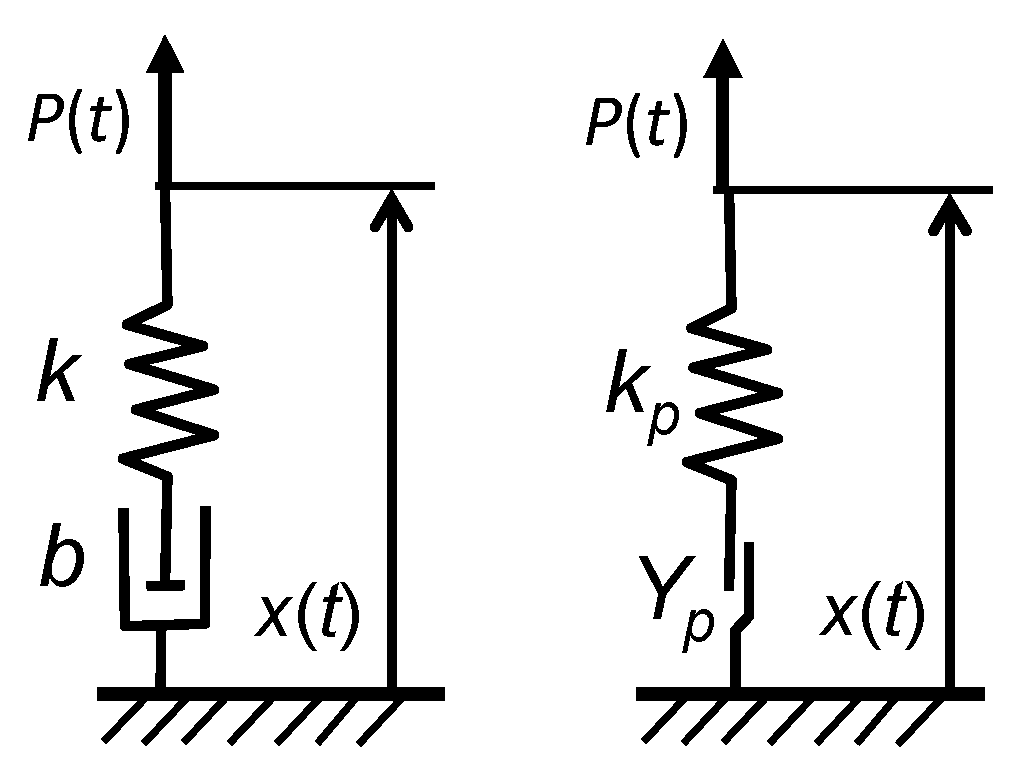
2.1. Modeling Energy Dissipation Considering Viscoelastic and Endochronic Material Behavior

The main difference between damping caused by viscoelastic elements (used to model rate-dependent material behavior) and damping caused by endochronic elements (used to model rate-independent material behavior) can easily be analyzed if hysteresis curves are compared. For this purpose, it is advantageous to concentrate on rheological models that have an identical topological structure, such as the Maxwell model (Figure 1, left) and the endochronic model (Figure 1, right).

Both models represent a serial connection, combining a linear elastic spring and a dissipative element. This leads to an additive decomposition of the total displacement $x$ into elastic and inelastic parts. The external force $P$ represents the system input to both systems. For the Maxwell element, we define an additive decomposition of $x$ into the elastic displacement $x_e$ and the displacement of the viscous dashpot $x_v$; compare (1). The elastic law is given by (2), where $k$ is the stiffness of the spring. The evolution of the viscous displacement is determined by (3), where $b$ is the viscosity of the dashpot.

$$x=x_e+x_v,$$

(1)

$$F=k{x}_e=k\left(x-x_v\right),$$

(2)

$${\dot{x}}_v=\frac{1}{b}F\hspace{0.17em}\hspace{0.17em}\hspace{0.17em}\mathrm{with}\hspace{0.17em}\hspace{0.17em}\hspace{0.17em}F=P.$$

(3)

For the endochronic element, the decomposition of $x$ is given by (4), where $x_p$ is the plastic displacement. The linear elastic law is given by (5), and the evolution of the inelastic deformation is described by (6), where the constant $Y$ has the dimension of a force. It should be noticed that using the endochronic theory of plasticity, the increment of plastic deformation $d{x}_p$ only depends on the increment of the total deformation $dx$ but not on the speed of the deformation process. For this reason, a rate-independent material behavior (without relaxation properties) is described by the endochronic approach.

$$x=x_e+x_p,$$

(4)

$$F=k{x}_e=k\left(x-x_p\right),$$

(5)

$${\dot{x}}_p=\frac{1}{Y}F\left|\dot{x}\right|\hspace{0.17em}\hspace{0.17em}\hspace{0.17em}\mathrm{with}\hspace{0.17em}\hspace{0.17em}\hspace{0.17em}F=P.$$

(6)

In the case of quasi-static tension, as well as considering the initial condition $x_p\left(0\right)=0$, it is possible to find a closed-form solution for the problem given by (4)–(6):

$$F=Y\left(1-e^{-\hspace{0.17em}\frac{k}{Y}x}\right).$$

(7)

The result shown in (7) proves that (without the further modeling of hardening effects) the constant $Y$ determines the maximum amount of force that can be transmitted though the endochronic element if the plastic flow is fully developed. It is also interesting to notice that a non-linear elastic law is described by (7). Thus, endochronic elements cannot be seen as linear time-invariant (LTI) systems that are (to the best knowledge of the author) reported clearly for the first time. However, assuming time–harmonic fluctuation for all quantities, it is possible to derive the following force–displacement relations for both rheological models:

$$\widehat{F}=\frac{j\mathsf{\Omega }k}{j\mathsf{\Omega }+k/b}\widehat{x},$$

(8)

$$\widehat{F}=\frac{jk}{j+\left(k/Y\right)\left|\widehat{x}\right|}\widehat{x},$$

(9)

where $\mathsf{\Omega }$ is the angular frequency, $\widehat{F}$ is the complex magnitude of the internal force $F$, $\widehat{x}$ is the complex magnitude of the total displacement $x$, and $j=\sqrt{-1}$ is the imaginary unit. While a rate-dependent material behavior is defined by (8) for the Maxwell element, a rate-independent material behavior is described by (9) for the endochronic element. To evaluate these two equations numerically, it is advantageous to introduce non-dimensional formulations such as

$$\tilde{\widehat{F}}=\frac{j\tilde{\mathsf{\Omega }}\tilde{k}}{j\tilde{\mathsf{\Omega }}+\tilde{k}/\tilde{b}}\tilde{\widehat{x}},$$

(10)

$$\tilde{\widehat{F}}=\frac{j\tilde{k}}{j+\left(\tilde{k}/\tilde{Y}\right)\left|\tilde{\widehat{x}}\right|}\tilde{\widehat{x}},$$

(11)

where a tilde indicates non-dimensional quantities in the non-dimensional formulations for the Maxwell element (10) and the endochronic element (11).

To define the normalized quantities given in (12), it is first necessary to choose reference values (${\omega }_0$ for the angular frequency, $x_0$ for the total displacement, and $k_0$- for the spring stiffness). Based on these reference values, it is then possible to define non-dimensional quantities such as

$$\tilde{\mathsf{\Omega }}:=\frac{\mathsf{\Omega }}{{\omega }_0},\hspace{0.17em}\hspace{0.17em}\hspace{0.17em}\tilde{k}:=\frac{k}{k_0},\hspace{0.17em}\tilde{\widehat{x}}:=\frac{\widehat{x}}{x_0},\hspace{0.17em}\hspace{0.17em}\tilde{\widehat{F}}:=\frac{\widehat{F}}{k_0{x}_0},\hspace{0.17em}\hspace{0.17em}\tilde{Y}:=\frac{Y}{k_0{x}_0},\hspace{0.17em}\hspace{0.17em}\hspace{0.17em}\mathrm{and}\hspace{0.17em}\hspace{0.17em}\tilde{b}:=\frac{b{\omega }_0}{k_0}.$$

(12)

Associated results for the cyclic loading are presented and discussed in Section 3.1.

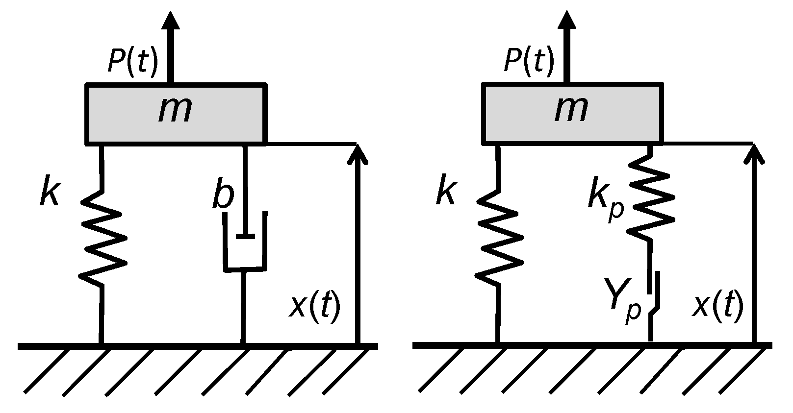
2.2. Vibration Models for Dynamic Systems with One Degree of Fredom

In order to compare the behavior of dynamic systems with viscoelastic damping on the one hand to the behavior of dynamic systems with endochronic damping mechanisms on the other hand, the classical harmonic oscillator (Figure 2, left) is compared to a one-degree-of-freedom system that considers an endochronic element (Figure 2, right).

In both systems, the displacement $x$ of the mass $m$ is caused by the external force $P$ that is reduced by a force $F_c$. Thus, the balance of linear momentum reads:

$$m\ddot{x}+kx=P-F_c\hspace{0.17em},$$

(13)

where the term $m\ddot{x}$ represents d’Alembert’s force (inertia force), while $kx$ is the elastic force in the spring with stiffness $k$; compare (13). Depending on the damping mechanism, the force $F_c$ is given by

$$F_c=b\dot{x},$$

(14)

in order to model the viscous force in the dashpot that is proportional to the vibration velocity(compare (14)) or, in case of the endochronic element, by the elastic law:

$$F_c=k_p\left(x-x_p\right),$$

(15)

where $k_p$ is the stiffness of the endochronic element, while the internal variable $x_p$ describes the amount of plastic displacement. The evolution of the internal variable $x_p$ (compare (15)), is given by the non-linear but rate-independent flow rule (16):

$${\dot{x}}_p=\frac{1}{Y_p}{F}_c\left|\dot{x}\right|,$$

(16)

where the constant $Y_p$ controls the evolution of the plastic deformation during the dynamic process. To develop a non-dimensional formulation for the equations of motion, it is necessary to introduce the dimensionless time $\tilde{t}$ such that

$$t\mapsto \tilde{t}:={\omega }_{0}t\hspace{0.17em}\hspace{0.17em}\hspace{0.17em}\mathrm{with}\hspace{0.17em}\hspace{0.17em}\hspace{0.17em}{\omega }_0:=\sqrt{k/m},$$

(17)

where ${\omega }_0$ is the natural angular frequency of the undamped system. As a consequence, the first- and second-time derivatives are given by

$$\frac{d(.)}{dt}={\omega }_0\frac{d(.)}{d\tilde{t}}=:{\omega }_0{(.)}^{\prime }\hspace{0.17em}\hspace{0.17em}\hspace{0.17em}\mathrm{and}\hspace{0.17em}\hspace{0.17em}\hspace{0.17em}\frac{d^2(.)}{d{\tilde{t}}^2}={\omega }_0^2\frac{d^2(.)}{d{\tilde{t}}^2}=:{\omega }_0^2{(.)}^{″}.$$

(18)

Furthermore, critical damping $D$, a non-dimensional stiffness ratio $v$, as well as non-dimensional displacements $\tilde{x}$ and ${\tilde{x}}_p$, a non-dimensional excitation force $\tilde{P}$, and the non-dimensional force constant ${\sigma }_p$ for the endochronic element are introduced such that

$$D:=\frac{b}{2\sqrt{km}},\hspace{0.17em}\hspace{0.17em}\hspace{0.17em}\hspace{0.17em}\nu :=\frac{k_p}{k},\hspace{0.17em}\hspace{0.17em}\hspace{0.17em}\hspace{0.17em}\tilde{x}:=\frac{x}{x_0},\hspace{0.17em}\hspace{0.17em}\hspace{0.17em}{\tilde{x}}_p:=\frac{x_p}{x_0},\hspace{0.17em}\hspace{0.17em}\hspace{0.17em}\tilde{P}:=\frac{P}{k{x}_0},\hspace{0.17em}\hspace{0.17em}\hspace{0.17em}{\sigma }_p:=\frac{k{x}_0}{Y_p},$$

(19)

where $x_0$ is a reference displacement. Considering these normalized quantities, defined in (19), the resulting non-dimensional equation of motion for the harmonic oscillator reads:

$${\tilde{x}}^{″}+2D{\tilde{x}}^{\prime }+\tilde{x}=\tilde{P},$$

(20)

while the set of non-dimensional equations of motion for the oscillator with the rate-independent endochronic element is given by

$${\tilde{x}}^{″}+\left(1+\nu \right)\tilde{x}-v{\tilde{x}}_p=\tilde{P}\hspace{0.17em}\hspace{0.17em}\hspace{0.17em}\mathrm{with}\hspace{0.17em}\hspace{0.17em}\hspace{0.17em}{{\tilde{x}}^{\prime }}_p=v{\sigma }_p\left(\tilde{x}-{\tilde{x}}_p\right)\left|{\tilde{x}}^{\prime }\right|.$$

(21)

It should be noticed that (19) represents a non-dimensional representation of an LTI system, while (20) and (21) describe a non-linear system because of the non-linear endochronic flow rule. The response of both systems is purely elastic if the relative velocity between the mass and the base tends to zero, because stress relaxation is not covered by the Kelvin model as well as by the endochronic model proposed in this study. For this reason, the simple Kelvin model is well suited as the rate-dependent reference model in the field of vibration control instead of the standard viscoelastic solid model that also includes the effect of stress relaxation.

Furthermore, the response of both systems is identical if damping can be neglected such that $D=0$ and the stiffness ratio is set to $v=0$. The impulse response, as well as the magnitude response of both system models, is discussed in Section 3.2.

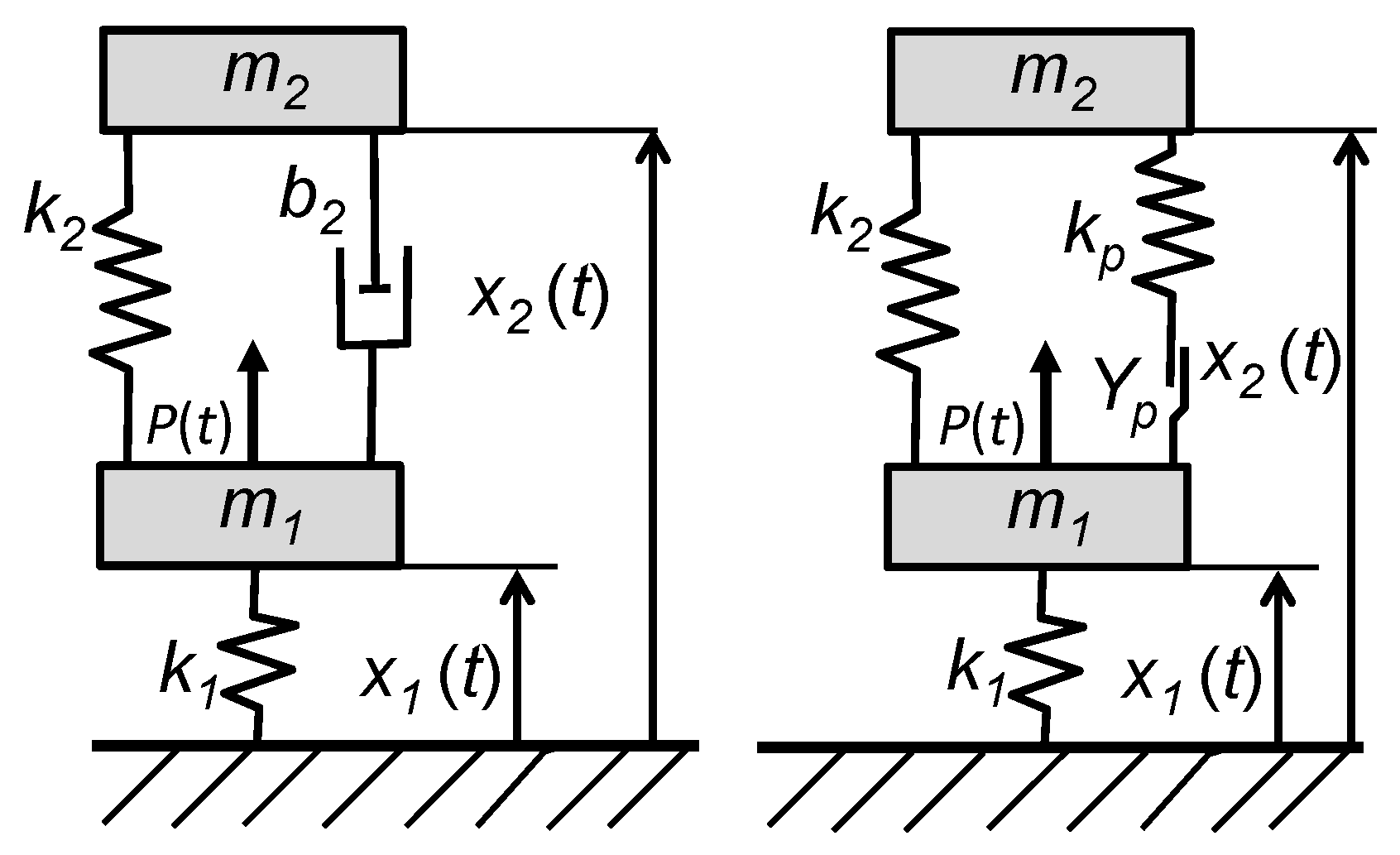
2.3. Vibration Models for Coupled Systems with Two Degrees of Freedom

Because the control of vibration by passive, semi-active or active systems requires a coupling between the vibrating system and the device used to attenuate the disturbance, it is necessary to analyze the dynamics of coupled systems. A situation in which two degrees of freedom have to be taken into account is shown in Figure 3, where the mass $m_1$ that is excited by the external force $P$ is coupled to vibration reduction devices. The latter are represented by the mass $m_2$. While a viscoelastic system is shown in Figure 3 (left), a non-linear endochronic system is presented in Figure 3 (right).

For both systems, the balance of linear momentum is given by (22) and (23), considering D’Alembert’s forces as well as linear elastic laws for every spring.

$$m_1{\ddot{x}}_1+\left(k_1+k_2\right)x_1-k_2{x}_2=P-F_c,$$

(22)

$$m_2{\ddot{x}}_2\hspace{0.17em}\hspace{0.17em}\hspace{0.17em}\hspace{0.17em}\hspace{0.17em}\hspace{0.17em}\hspace{0.17em}\hspace{0.17em}\hspace{0.17em}\hspace{0.17em}\hspace{0.17em}\hspace{0.17em}\hspace{0.17em}\hspace{0.17em}\hspace{0.17em}-k_2{x}_1+k_2{x}_2=\hspace{0.17em}\hspace{0.17em}\hspace{0.17em}\hspace{0.17em}\hspace{0.17em}\hspace{0.17em}\hspace{0.17em}\hspace{0.17em}\hspace{0.17em}\hspace{0.17em}{F}_c.$$

(23)

However, as for the single degree of freedom systems, the definition of the force $F_c$ depends on the damping mechanism that has to be described. In the case of viscoelastic damping, this quantity is given by the relative velocity in the dashpot, as shown in (24).

$$F_c=b\left({\dot{x}}_2-{\dot{x}}_1\right).$$

(24)

If damping is modeled using the rate-independent endochronic approach, the force $F_c$ is given by the elastic law (25), while the evolution of the plastic displacement $x_p$ is described by the flow rule (26).

$$F_c=k_p\left(x_2-x_1-x_p\right),$$

(25)

$${\dot{x}}_p=\frac{1}{Y_p}{F}_c\left|{\dot{x}}_2-{\dot{x}}_1\right|.$$

(26)

Considering an elastic coupling between $m_1$ and $m_2$, the force $F_c$ could also be applied by a proper actuator (compare Figure 4 (left)) driven by the control signal $u$. The latter is calculated by the controller $C$ based on sensor signals. These are the transducer force $F_p$ and the measure of the relative velocity ${\dot{x}}_2-{\dot{x}}_1$, which can also be integrated into the control unit (compare Figure 4 (right)). This remark is important, because it answers the question of how endochronic elements can be realized in practical applications. By using an approach that is based on active control, it is not necessary to rely on materials with specific properties or to consider a limit for plastic deformation to ensure the integrity of the structural design. One practical example for the electronic representation of the physical properties used for vibration reduction has recently been proposed in [24]. The control law for the endochronic approach is shown in Figure 4 (right). It can be easily implemented with an appropriate signal processing hardware.

However, the main intention of this contribution is to analyze the noise control potential of viscoelastic and endochronic noise control devices attached to a dynamic system in a general way. To proceed, it is again advantageous to develop a non-dimensional version of the equations of motion. At first, the non-dimensional time $\tilde{t}$ is redefined, considering the angular frequency ${\omega }_1$ as shown in (27):

$$\tilde{t}:={\omega }_{1}t\hspace{0.17em}\hspace{0.17em}\hspace{0.17em}\hspace{0.17em}\mathrm{with}\hspace{0.17em}\hspace{0.17em}\hspace{0.17em}\hspace{0.17em}{\omega }_1:=\sqrt{k_1/m_1}.$$

(27)

As a consequence, the first- and second-time derivatives are now given by

$$\frac{d(.)}{dt}={\omega }_1\frac{d(.)}{d\tilde{t}}=:{\omega }_1{(.)}^{\prime }\hspace{0.17em}\hspace{0.17em}\hspace{0.17em}\mathrm{and}\hspace{0.17em}\hspace{0.17em}\hspace{0.17em}\frac{d^2(.)}{d{\tilde{t}}^2}={\omega }_1^2\frac{d^2(.)}{d{\tilde{t}}^2}=:{\omega }_1^2{(.)}^{″},$$

(28)

for both degrees of freedom. Furthermore, it is necessary to define a mass ratio as well as to introduce two modified stiffness ratios, such as those presented in (29):

$$\mu {\lambda }^2:=\sqrt{k_2/k_1},\hspace{0.17em}\hspace{0.17em}\hspace{0.17em}\mathrm{and}\hspace{0.17em}\hspace{0.17em}\hspace{0.17em}\hspace{0.17em}\hspace{0.17em}\mu {\lambda }_p^2:=\sqrt{k_p/k_1}\hspace{0.17em}\hspace{0.17em}\hspace{0.17em}\hspace{0.17em}\mathrm{with}\hspace{0.17em}\hspace{0.17em}\hspace{0.17em}\mu :=\sqrt{m_2/m_1}\hspace{0.17em}.$$

(29)

Critical damping is now defined by (30):

$$D:=\frac{b_2}{2\sqrt{k_1{m}_1}}\hspace{0.17em}.$$

(30)

Furthermore, non-dimensional variables for the external force and the two degrees of freedom are introduced in (31):

$$\tilde{P}:=\frac{P}{k_1{x}_0},\hspace{0.17em}\hspace{0.17em}\hspace{0.17em}{\tilde{x}}_1:=\frac{x_1}{x_0},\hspace{0.17em}\hspace{0.17em}\hspace{0.17em}{\tilde{x}}_2:=\frac{x_2}{x_0},$$

(31)

where $\hspace{0.17em}{x}_0$ is again a reference displacement. Finally, the non-dimensional constant for the endochronic element has to be re-defined such that

$${\sigma }_p:=\frac{x_0{k}_1}{Y_p}.$$

(32)

Using the definitions given by (27)–(32), it is possible to derive the following sets of non-dimensional equations. At first, the non-dimensional model of the viscoelastic system (compare Figure 3, left) is presented in (33):

$$\left[\begin{array}{cc}1& 0\\ 0& \mu \end{array}\right]\left[\begin{array}{c}{\tilde{x}}_1^{″}\\ {\tilde{x}}_2^{″}\end{array}\right]+2D\left[\begin{array}{cc}1& -1\\ -1& 1\end{array}\right]\left[\begin{array}{c}{\tilde{x}}_1^{\prime }\\ {\tilde{x}}_2^{\prime }\end{array}\right]+\left[\begin{array}{cc}1+\mu {\lambda }^2& -\mu {\lambda }^2\\ -\mu {\lambda }^2& +\mu {\lambda }^2\end{array}\right]\left[\begin{array}{c}{\tilde{x}}_1\\ {\tilde{x}}_2\end{array}\right]=\left[\begin{array}{c}\tilde{P}\\ 0\end{array}\right].$$

(33)

The non-dimensional model for the two degrees of freedom system with the endochronic element (compare Figure 3, right) is given by

$$\left[\begin{array}{cc}1& 0\\ 0& \mu \end{array}\right]\left[\begin{array}{c}{\tilde{x}}_1^{″}\\ {\tilde{x}}_2^{″}\end{array}\right]+\left[\begin{array}{cc}1+\mu \left({\lambda }^2+{\lambda }_p^2\right)& -\mu \left({\lambda }^2+{\lambda }_p^2\right)\\ -\mu \left({\lambda }^2+{\lambda }_p^2\right)& +\mu \left({\lambda }^2+{\lambda }_p^2\right)\end{array}\right]\left[\begin{array}{c}{\tilde{x}}_1\\ {\tilde{x}}_2\end{array}\right]+\mu {\lambda }_p^2\left[\begin{array}{c}1\\ -1\end{array}\right]{\tilde{x}}_p=\left[\begin{array}{c}\tilde{P}\\ 0\end{array}\right],$$

(34)

where the evolution equation for the non-dimensional plastic displacement is defined by (35) such that

$${{\tilde{x}}^{\prime }}_p=\mu {\lambda }_p^2{\sigma }_p\left({\tilde{x}}_2-{\tilde{x}}_1-{\tilde{x}}_p\right)\left|{\tilde{x}}_2^{\prime }-{\tilde{x}}_1^{\prime }\right|.$$

(35)

The models defined by (33) as well as by (34) and (35) can be used to analyze the behavior of both systems numerically. It should be noticed that (33) represents a time-domain model of an LTI system, while the set of equations summarized in (34) and (35) describe a non-linear system. The response of both systems is identical if damping can be neglected, i.e., $D=0$ and ${\lambda }_p=0$. It is easy to prove that for the time–harmonic fluctuation of all quantities, a frequency-domain representation can be derived from (33) for the viscoelastic system that is given in (36):

$$\left[\begin{array}{cc}1+\mu {\lambda }^2-{\tilde{\mathsf{\Omega }}}^2+j2D\tilde{\mathsf{\Omega }}& -\mu {\lambda }^2-j2D\tilde{\mathsf{\Omega }}\\ -\mu {\lambda }^2-j2D\tilde{\mathsf{\Omega }}& \mu \left({\lambda }^2+{\tilde{\mathsf{\Omega }}}^2\right)+j2D\tilde{\mathsf{\Omega }}\end{array}\right]\left[\begin{array}{c}{\tilde{\widehat{x}}}_1\\ {\tilde{\widehat{x}}}_2\end{array}\right]=\tilde{\widehat{P}}\left[\begin{array}{c}1\\ 0\end{array}\right],$$

(36)

where a hat indicates the complex magnitude of a non-dimensional quantity. However, if (25) is not used to eliminate the force $F_c$ in the balance of linear momentum (22) and (23), it is, after some algebraic manipulations, also possible to derive a non-linear frequency-domain model for time–harmonic analysis of the system with the endochronic element such that

$$\left[\begin{array}{cc}1+\mu {\lambda }^2-{\tilde{\mathsf{\Omega }}}^2& -\mu {\lambda }^2\\ -\mu {\lambda }^2& \mu \left({\lambda }^2+{\tilde{\mathsf{\Omega }}}^2\right)\end{array}\right]\left[\begin{array}{c}{\tilde{\widehat{x}}}_1\\ {\tilde{\widehat{x}}}_2\end{array}\right]=\tilde{\widehat{P}}\left[\begin{array}{c}1\\ 0\end{array}\right]+{\tilde{\widehat{F}}}_c\left[\begin{array}{c}1\\ -1\end{array}\right],$$

(37)

where the complex magnitude of the non-dimensional force ${\tilde{\widehat{F}}}_c$ is given by

$${\tilde{\widehat{F}}}_c=\frac{j\mu {\lambda }_p^2\cdot \left({\tilde{x}}_2-{\tilde{x}}_1\right)}{j+\mu {\lambda }_p^2{\sigma }_p\cdot \left|{\tilde{x}}_2-{\tilde{x}}_1\right|}.$$

(38)

With (37) and (38), the present paper proposes, for the first time, a non-linear and non-dimensional model of coupled dynamical systems that enables an efficient way of analyzing vibration control with endochronic elements that considers time–harmonic excitation in the frequency domain. Thus, following this approach, numerical integration of the equations of motion is not necessary for time–harmonic excitation signals. This is an important finding, because optimizing model parameters becomes more efficient if algebraic equations have to be solved instead of ODEs. The time-domain models as well as the frequency-domain system representations have been used for numerical investigations. The associated results are presented in Section 3.3.

3. Results of Numerical Investigations and Discussion of Noise-Control Potential

3.1. Energy Dissipation Described by Viscoelastic and Endochronic Rheological Models

The analytical models (10) and (11) derived for the Maxwell element (Figure 1, left) and the endochronic element (Figure 1, right) have been analyzed by considering two normalized angular frequencies, ${\tilde{\mathsf{\Omega }}}_1=0.75$ and ${\tilde{\mathsf{\Omega }}}_2=1.25$; compare (12). Furthermore, the following non-dimensional constants have been used to specify the non-dimensional stiffness, the non-dimensional viscosity, and the non-dimensional force such that $\tilde{k}=\hspace{0.17em}\hspace{0.17em}100.0$, $\tilde{b}=\hspace{0.17em}\hspace{0.17em}15.0$, $\tilde{Y}=\hspace{0.17em}\hspace{0.17em}100.0$.

The simulation results for the endochronic element are shown in Figure 5 (left), while the results for the Maxwell element are presented in Figure 5 (right). As illustrated by Figure 5 (left), rate-independent material behavior is described by the endochronic element, because the shape of the hysteresis curves is independent of frequency.

The presented results also prove that both the magnitude response as well as the phase response of the endochronic element described by (11) are independent of frequency. This is an interesting result that is presented in this form for the first time. The same is, however, not true for the Maxwell element (compare Figure 5 (right)), which can be applied to model rate-dependent hysteresis effects as well as relaxation and creep into quasi-static deformation processes.

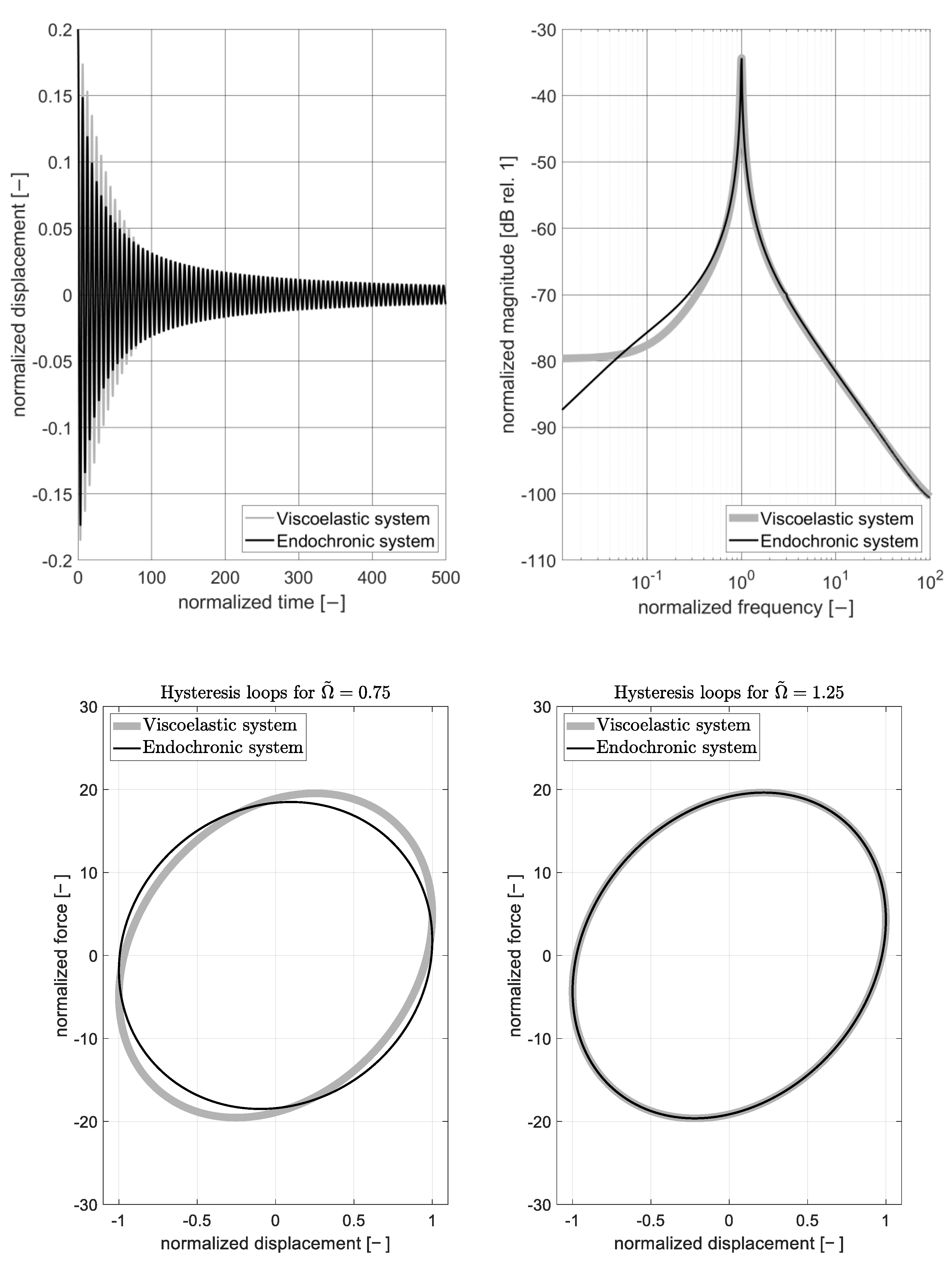
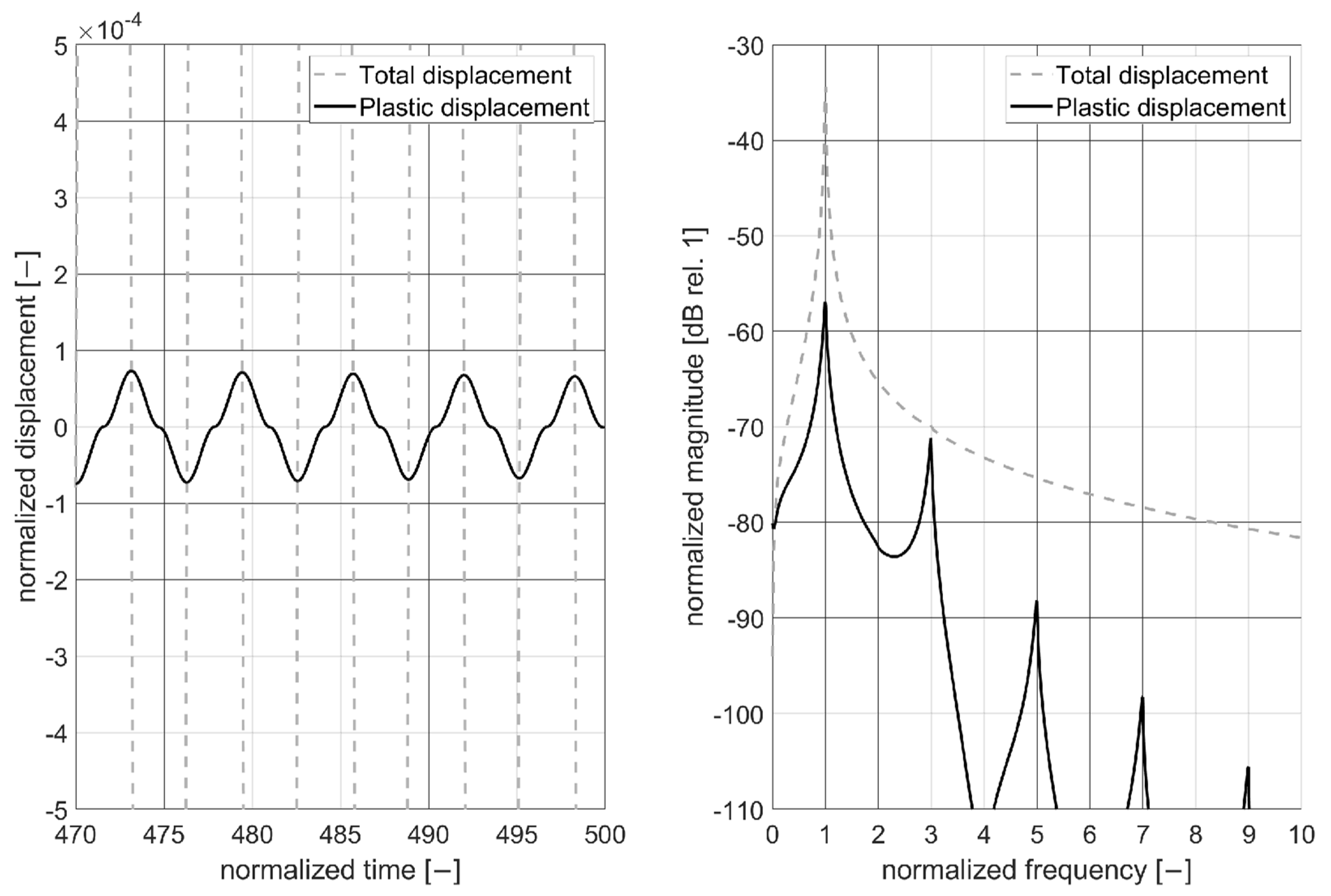
3.2. Dynamic Behavior of Systems with One Degree of Freedom

In order to study the behavior of dynamic systems with viscoelastic damping and dissipation caused by plastic deformation, the mathematical models for the harmonic oscillator (20) and the oscillator with an endochronic element (21) have been analyzed numerically, considering a unit impulse as the system input such that $\tilde{P}\left(0\right)=1.0$. A self-implemented fourth-order Runge–Kutta scheme with a fixed step size has been applied to numerical integration, considering 25,000 time steps. To apply the Runge–Kutta schema, the set of equations has been transformed to a set of ODEs containing only first derivatives with respect to the non-dimensional time $\tilde{t}$. All initial conditions have been set to zero. To fulfill the Nyquist–Shannon sampling theorem (where the sample rate must be twice the bandwidth of the signal), the non-dimensional sampling frequency has been set to ${\tilde{f}}_s=50.0\cdot {\tilde{f}}_0$, where ${\tilde{f}}_0=1.0$ is the normalized resonance frequency, according to (17).

For the harmonic oscillator described by (20), critical damping has been set to $D=0.02$. In order to match the resonance of the harmonic oscillator, the system parameters of the non-linear oscillator described by (21) have been set to $v=0.5$ and σ_p = 5.0. The associated simulation results are presented in Figure 6 and Figure 7.

For both systems, the impulse response curves are shown in Figure 6 (top left), while the normalized magnitude response curves are presented in Figure 6 (top right) using a semi-logarithmic scale. As typical for viscoelastic systems, an exponential decay of the normalized displacement has been simulated for the model of the harmonic oscillator (compare Figure 6 (top left)). A significant (but not exponential) decay of the impulse response has also been found for the non-linear oscillator with the endochronic element, compare Figure 6 (top left). Furthermore, hysteresis loops are shown in Figure 6, considering $\tilde{\mathsf{\Omega }}=0.75$ as one example for a normalized frequency below the natural frequency (Figure 6 (bottom left)), and $\tilde{\mathsf{\Omega }}=1.25$ as one example for a normalized frequency above the natural frequency (Figure 6 (bottom right)). These figures simply show that the hysteresis loops of the oscillator with an endochronic element can be designed to be equivalent to the hysteresis loops of the classical harmonic oscillator.

The magnitude response curves of both systems are nearly identical for normalized frequencies above the resonance (compare Figure 6 (right)). It should be noticed that for quasi-static excitation (low normalized frequencies below the resonance), the force transmitted though the dashpot of the harmonic oscillator is close to zero. For this reason, the magnitude response of the system described by (20) covers a static deflection for very low normalized frequencies. This is not true for the non-linear system described by (21), because the force transmitted through the endochronic element is rate-independent, as discussed in the previous subsection. For this reason, a plastic flow is also induced at very low normalized frequencies and causes an attenuation of the excitation that can be observed in the magnitude response curve (compared in Figure 6 (right)).

In order to illustrate the non-linear effects caused by the endochronic element that have also been discussed for static loading, the reader is referred to the discussion in (7). The evolution of the plastic displacement is shown in Figure 7 (left), considering a small section of the time series. It is interesting to note that the evolution of the plastic displacement is a non-linear process. The higher harmonics that contribute to the evolution of the plastic displacement are uneven multiples of the normalized natural frequency. In particular, the first higher harmonic contributes significantly to the time-domain response of the endochronic element. For the chosen set of parameters, the non-linear characteristic is not to be found in the frequency response of the total displacement; compare Figure 7 (right).

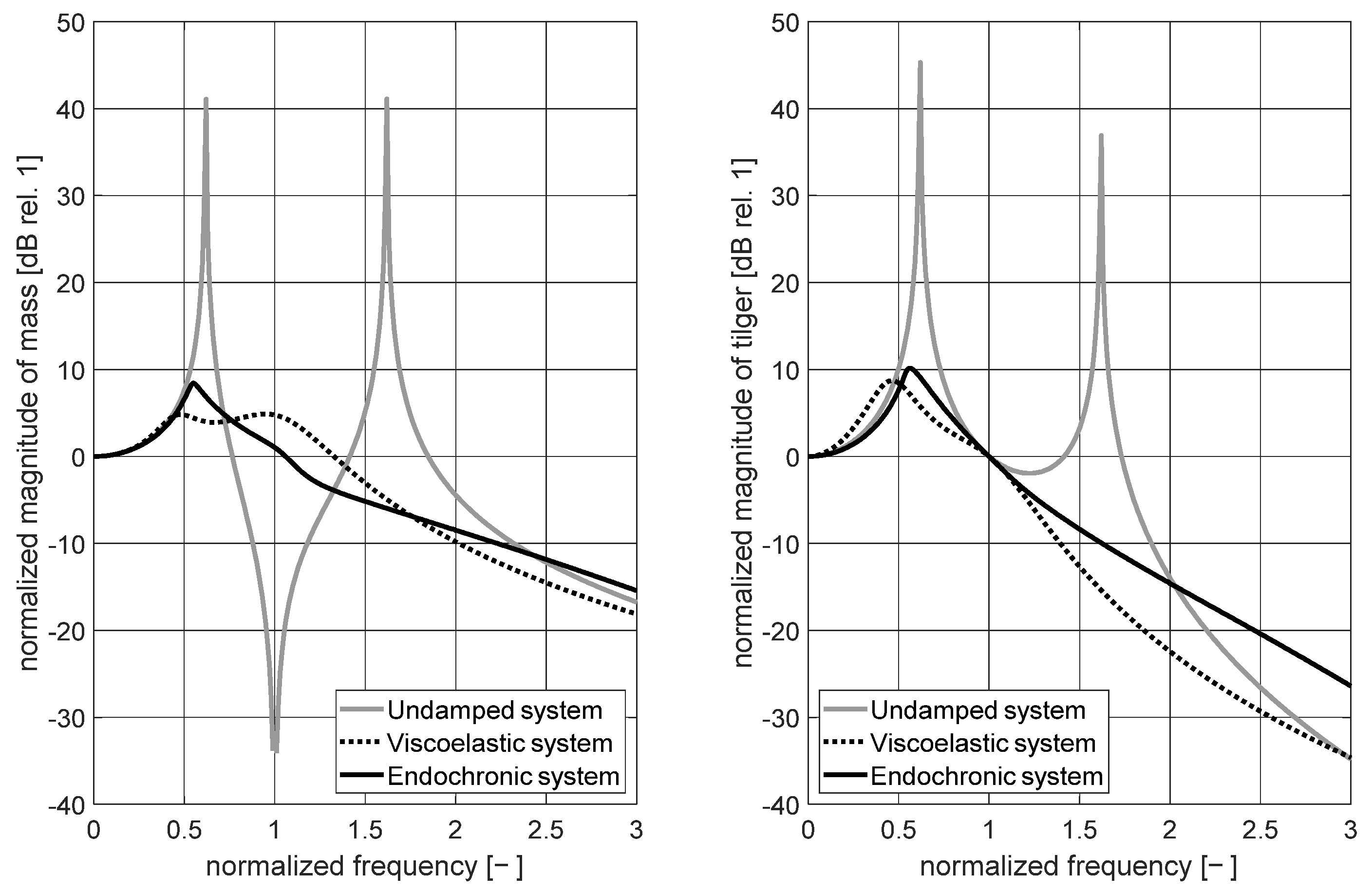
3.3. Discussion of Dynamic Behavior and Evaluation of Control Profit for Coupled Systems

In order to evaluate the vibration control potential of dynamic absorbers that are based on viscoelastic and plastic dissipation, it is necessary to analyze the dynamical behavior of coupled systems. In the present contribution, the DA is used as a reference (compare Figure 3 (left)). Its time-domain representation is given by (33), while the associated frequency-domain model is given by (36). The CP, which can be obtained by the application of an optimally tuned DA (compare with (42)), is compared to the CP that is estimated for an optimally tuned endochronic absorber (EA) (compare Figure 3 (right)). The time-domain model for the coupled system with the EA is given by (34) and (35). Its frequency-domain counterpart is given by (37) and (38).

As in the previous subsection, a self-implemented fourth-order Runge–Kutta schema with fixed step size has been used to perform numerical integrations for another 50,000 time steps, considering initial conditions that have been set to zero for all quantities. To fulfill Shannon’s criteria, the non-dimensional sampling frequency has been set to ${\tilde{f}}_s=10.0 {\tilde{f}}_1$, where ${\tilde{f}}_1=1.0$ is a normalized frequency according to (27). For both models, the mass ratio has been set to $\mu =1.0$. The optimal values for the DA (compare with (39)) have been calculated following the procedure proposed in [1].

$$D_{opt}=\sqrt{3{\mu }^3/8{\left(1+\mu \right)}^3}=0.21,\hspace{0.17em}\hspace{0.17em}\hspace{0.17em}{\lambda }_{opt}=1/\left(1+\mu \right)=0.5.$$

(39)

To simulate the EA, the stiffness ratio $\lambda$ has been set to the optimal value of the DA given in (39) such that $\lambda ={\lambda }_{opt}=0.5$. The remaining normalized constants for the endochronic element have been set to

$${\lambda }_{p,}{}_{opt}=1.41\hspace{0.17em}\hspace{0.17em}\hspace{0.17em}\mathrm{and}\hspace{0.17em}\hspace{0.17em}\hspace{0.17em}{\sigma }_{p,}{}_{opt}=1.38.$$

(40)

The constants given in (40) have been determined by genetic optimization, limiting the parameter space for both constants by the lower boundary 0.0 and the upper boundary 2.0. The cost function (41) that has been applied to find these constants (defining an optimally tuned EA) has been defined as the sum of the squared normalized magnitudes of the system mass $m_1$ and the so called tilger mass $m_2$ such that

$$\underset{{\lambda }_p,{\sigma }_p}{\mathrm{minimize}}J\left({\lambda }_p,{\sigma }_p\right)\hspace{0.17em}\hspace{0.17em}\hspace{0.17em}\mathrm{with}\hspace{0.17em}\hspace{0.17em}\hspace{0.17em}J\left({\lambda }_p,{\sigma }_p\right):={\displaystyle \sum _{i=1}^{i=301}{\left|{\tilde{\widehat{x}}}_1\left(j{\tilde{\mathsf{\Omega }}}_i\right)\right|}^2+{\left|{\tilde{\widehat{x}}}_2\left(j{\tilde{\mathsf{\Omega }}}_i\right)\right|}^2},$$

(41)

considering 300 normalized frequencies in the range $\tilde{\mathsf{\Omega }}\in \left(0,3\right)$. To solve the non-linear set of equations given by (37) and (38), the Levenberg–Marquardt algorithm has been applied. The results calculated for the optimally tuned DA and the optimally tuned EA will be compared to results that have been calculated for a system without damping, considering only the system mass $m_1$ and the tilger mass $m_2$, the two springs characterized by $k_1$ and $k_2$, as well as the ratios $\mu =1.0$ and $\lambda =1.0$.

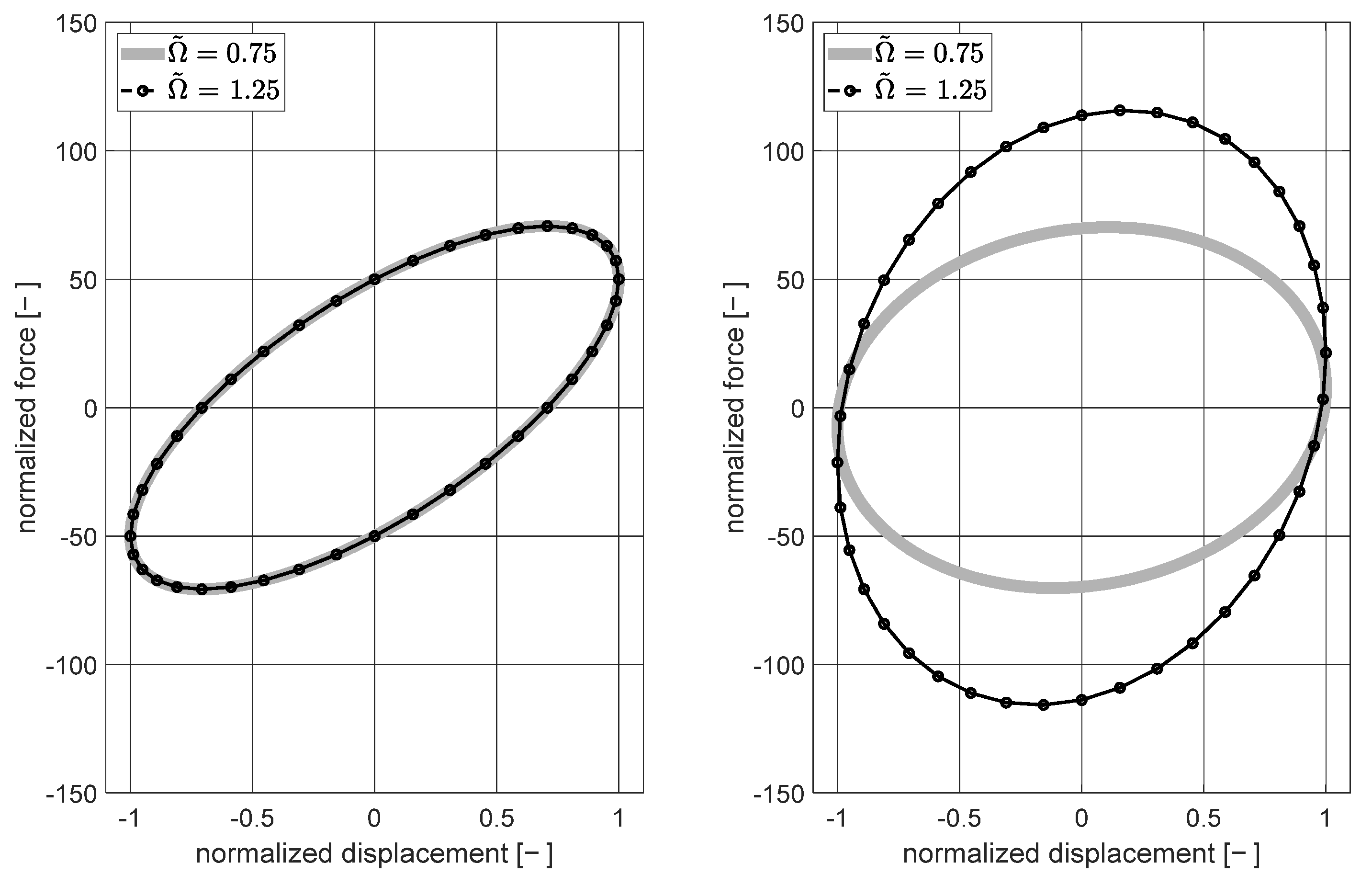
3.3.1. Time–Harmonic Analysis of Coupled Systems

Numerical results obtained for (i) the undamped system, (ii) the optimally tuned DA, and (iii) the optimally tuned EA considering the time–harmonic excitation acting on the system mass $m_1$ are presented in Figure 8. The normalized response of the system mass $m_1$ due to excitation acting on the system mass $m_1$ is shown in Figure 8 (left). The curve indicating the system without damping illustrates three characteristic frequencies. These are the two resonance frequencies that are located at ${\tilde{\mathsf{\Omega }}}_{R1}=0.62$ and ${\tilde{\mathsf{\Omega }}}_{R2}=1.62$ as well as the anti-resonance that is to be found at ${\tilde{\mathsf{\Omega }}}_T=1.0$. The latter is identical to the normalized natural frequency of the undamped single degree of freedom system.

The normalized magnitude response of the tilger mass $m_2$ caused by the excitation acting on $m_1$ is shown in Figure 8 (right). The resonance frequencies ${\tilde{\mathsf{\Omega }}}_{R1}$ and ${\tilde{\mathsf{\Omega }}}_{R2}$ can also be detected in the associated curve.

This is not possible by following the response curves representing the systems with the optimally tuned DA and the optimally tuned EA, because a significant and broadband reduction of the vibration level is simulated for both approaches. Furthermore, as known from the theory of mechanical vibrations, the effect of damping lowers the CP outside the resonances—especially around the anti-resonance.

It should be noticed that by using the set of parameters determined for the optimally tuned DA and the optimally tuned EA, the CP realized with the DA exceeds the CP that is realized with the EA around the resonance frequencies. However, the results presented in Figure 8 (left) also prove that the increase in vibration level around the anti-resonance is lower if the EA is used to attenuate the vibration at the system mass $m_1$.

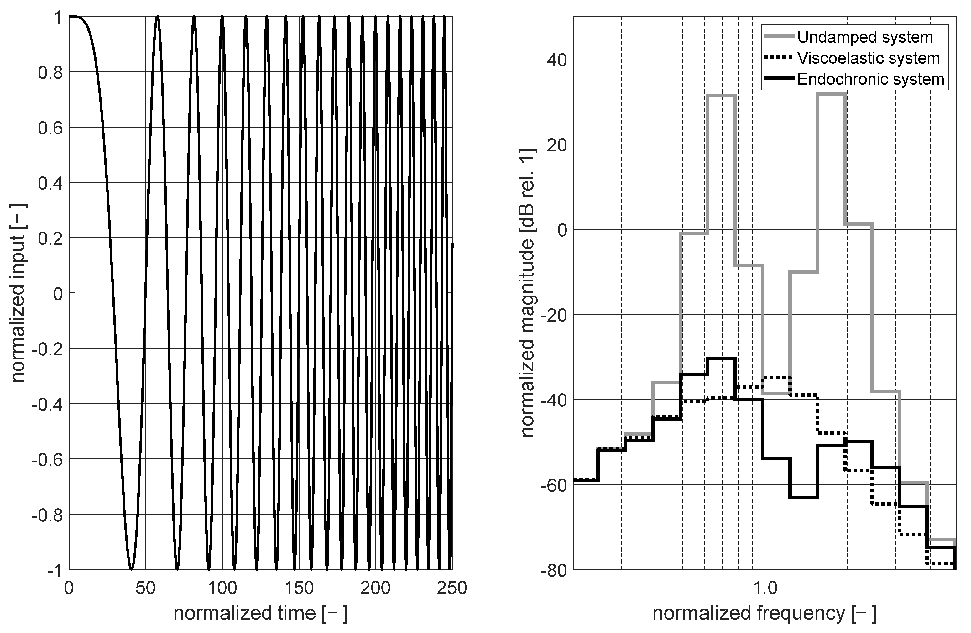
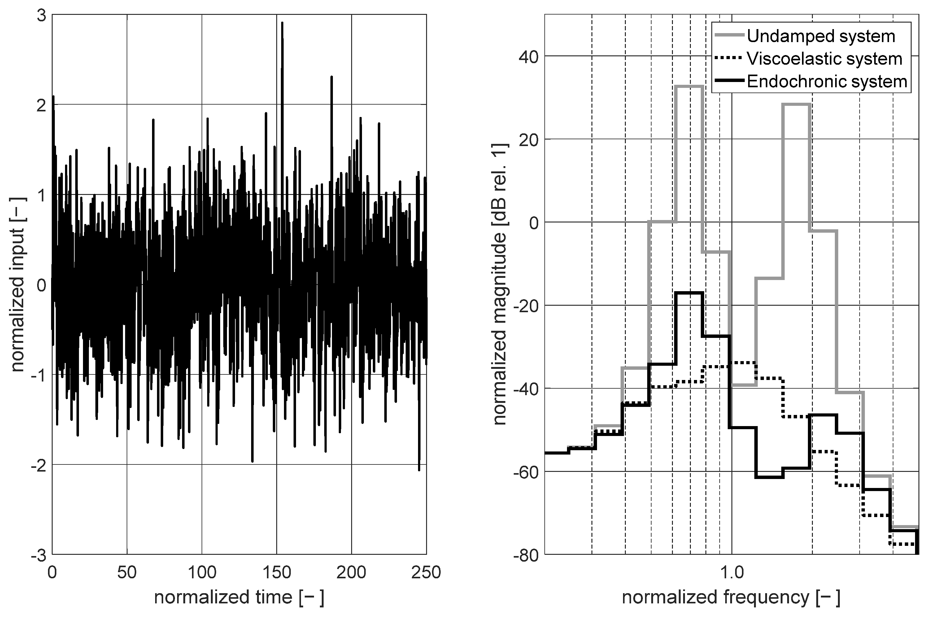
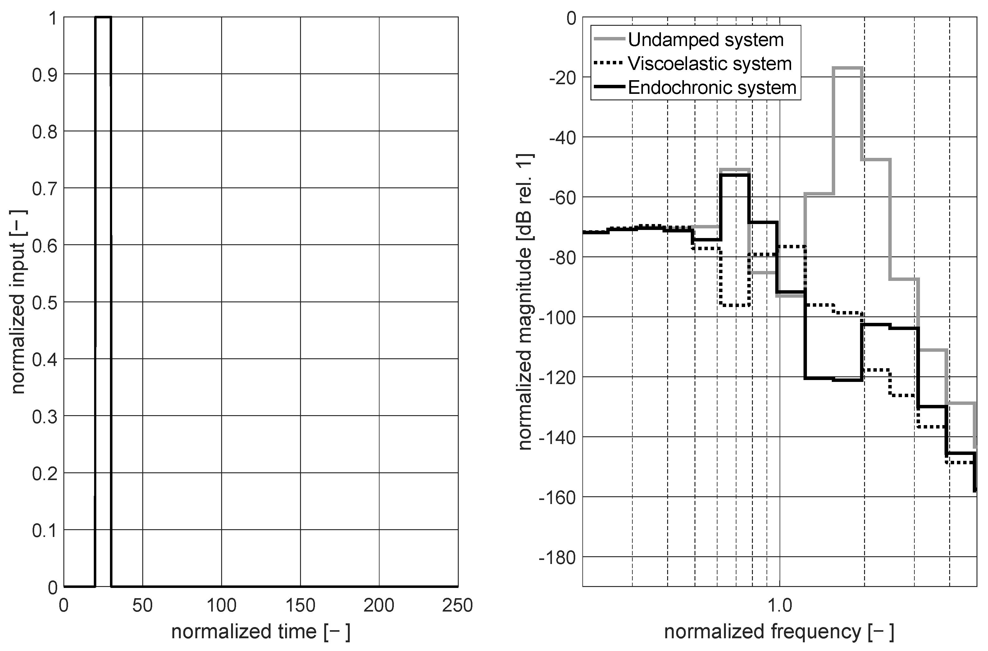
3.3.2. System Analysis Considering Broadband and Time-Varying Excitation Signals

In order to analyze the response of coupled systems caused by more sophisticated input signals, numerical simulations have also been performed using (i) a linear chirp signal, (ii) white Gaussian noise, and (iii) a step signal as the system input. However, in contrast to the results of the time–harmonic analysis presented in Figure 8, the magnitude response is now presented as a 1/3 octave-band analysis. For this purpose, the octave bands defined in [25] have been used, considering an upscaling of the normalized sampling frequency by a factor of 1000 by calculating the 1/3 octave-band analysis using the Matlab^® command “poctave”.

Furthermore, all 1/3 octave-band plots have been adjusted by multiplying the data on the x-aches by the factor 6.2 in order to match the anti-resonance ${\tilde{\mathsf{\Omega }}}_T=1.0$ in the normalized representation for the non-dimensional frequency range. Because the CP is especially relevant for the system mass $m_1$ the 1/3 octave-band analysis has been limited to the magnitude response of the normalized displacement ${\tilde{x}}_1$.

Figure 9 presents numerical results that have been obtained by analyzing the dynamics of coupled systems using a linear chirp as the input signal. The latter has been designed in such a way that the maximum value of the normalized frequency $\max (\tilde{\mathsf{\Omega }})=3$ is reached at the end of the simulation. Figure 9 (left) presents this input signal, considering the first 5% of the total time scale. The associated 1/3 octave-band response curves of the system mass $m_1$ are shown in Figure 9 (right), considering the full time scale.

As for the excitation with time–harmonic signals, it is possible to identify the two resonance frequencies ${\tilde{\mathsf{\Omega }}}_{R1}=0.62$ and ${\tilde{\mathsf{\Omega }}}_{R2}=1.62$ as well as the anti-resonance at ${\tilde{\mathsf{\Omega }}}_T=1.0$ by analyzing the curve for the undamped system.

Furthermore, it is possible to validate that vibration control based on an optimally tuned DA lowers the magnitude response around the resonance frequencies but increases the magnitude response around the anti-resonance. The application of an optimally tuned EA improves the CP at the anti-resonance. But the CP obtained around the resonance frequency is smaller compared with the CP that is obtained by the application of an optimally tuned DA. However, by comparing the results presented in Section 3.3.1 to the results presented in Section 3.3.2, it must be taken into account that Fourier spectra are presented in Section 3.3.1, while 1/3 octave-band power spectra are presented in Section 3.3.2.

Numerical results that have been obtained by simulating the system response using white Gaussian noise as the input signal are presented in Figure 10. The input signal is shown in Figure 10 (left) for the first 5% of the total time scale. The associated 1/3 octave-band response curves of the system mass $m_1$ are shown in Figure 10 (right). These results are in very good agreement with the results presented in Figure 9 (right). Small deviations in magnitude are caused by the fact that only one (time-limited) realization of a stochastic process has been considered. The data are therefore not identical to results obtained by using deterministic signals, even if an identical frequency range is excited.

Figure 11 presents results that have been obtained by analyzing the response of coupled systems that consider a step input signal. The latter is shown in Figure 11 (left). It is both deterministic and broadband but can also be classified as transient. It has been considered in order to investigate the response to a short time and non-stationary excitation signal. In contrast to the input signal shown in Figure 11 (left), the chirp signal shown in Figure 9 (left) changes relatively slowly in time. Furthermore, the white Gaussian noise signal shown in Figure 10 (left) can be classified as a stationary signal that enables the system that is excited to generate a stationary response (known as forced vibration) if the amount of damping is significant.

The 1/3 octave-band magnitude response curves caused by the step input signal are shown in Figure 11 (right). Because of the transient character of the input signal, these results differ from the results shown in Figure 9 (right) and Figure 10 (right).

It can be seen that the CP around the resonances is more significant if the optimally tuned DA is coupled to the system’s mass $m_1$. This is especially true for ${\tilde{\mathsf{\Omega }}}_{R1}=0.62$. However, it is easy to explain why the CP realized with the optimally tuned EA is in the same range of magnitude compared to the CP realized with the optimally tuned DA around ${\tilde{\mathsf{\Omega }}}_{R2}=1.62$. In order to generate plastic dissipation, a relative motion is required between the system’s mass $m_1$ and the tilger mass $m_2$. This relative motion is more significant for a mode shape in which both masses vibrate out-of-phase.

This is typical for the second resonance frequency ${\tilde{\mathsf{\Omega }}}_{R2}$ but not for the first resonance frequency ${\tilde{\mathsf{\Omega }}}_{R1}$. Thus, it can be concluded that the short-time step input used in this analysis is more capable of exciting the out-of-phase vibration instead of the first mode shape that is characterized by an in-phase displacement of the system mass $m_1$ and tilger mass $m_2$.

Nevertheless, it has been found that the application of an optimally tuned EA also enables a significant CP if the excitation signal has a transient character. An amplification of the dynamic response around resonances has not been detected.

3.3.3. Discussion of Noise-Control Potential

In order to discuss the noise-control potential, it is necessary to define an appropriate measure for the CP. The latter can be established as the difference between the overall vibration level of the uncontrolled and the controlled system such that

$$CP:=L_{\Sigma ,\mathrm{uncontrolled}}-L_{\Sigma ,\mathrm{controlled}},$$

(42)

where the overall vibration level for the uncontrolled system $L_{\Sigma ,\mathrm{uncontrolled}}$ and the overall level for the controlled system $L_{\Sigma ,\mathrm{controlled}}$ (compare (42)) have to be calculated according to the usual approach.

$$L_{\Sigma }=10\cdot {\log }_{10}\left(\frac{y_1^2+y_2^2+\dots +y_N^2}{y_0^2}\right),$$

(43)

considering a proper reference value $y_0$. Following this approach, the CP has been evaluated for all types of input signals.

Table 1. Overall control profit for different excitation signals shown for the optimally tuned dynamic absorber (DA) and the optimally tuned endochronic absorber (EA).

Type of Input Signal	Control Profit DA	Control Profit EA
sine	19.7 dB	20.9 dB
chirp	65.0 dB	62.9 dB
white Gaussian noise	58.8 dB	46.6 dB
shock	46.9 dB	35.4 dB

contains the numerical data that have been calculated for every frequency line (sine) and every 1/3 octave-band frequency (chirp, white Gaussian noise, step). However, by comparing the absolute values, it must be taken into account that the results obtained from the time–harmonic analysis (sine) are taken from a narrow-band Fourier spectrum, while the results obtained for all remaining input signals are evaluated as 1/3 octave-band power spectra.

The results shown in Table 1 (first row) prove that the overall CP is nearly identical if the time–harmonic excitation is relevant as the system input. This finding is in fair agreement with the results presented in Figure 8 (left). The data presented in the second, third, and fourth row prove that a significant CP can be achieved if optimally tuned absorbers are applied. Also, these data are in good agreement with the simulation results presented in Figure 9 (right), Figure 10 (right), and Figure 11 (right).

It can be concluded that the CP is reduced if the system input becomes stochastic and transient. For the chirp signal, the CP obtained with the optimally tuned EA is nearly identical to the CP that is obtained with the optimally tuned DA. However, if random excitation and shock are considered, the overall CP obtained with the optimally tuned EA is still significant, even if the overall CP obtained with the optimally tuned DA has a benefit close to 12 dB.

If an electronic realization of the control approach is applied (compare Figure 4), it is also possible to switch between the characteristics of an optimally tuned DA and an optimally tuned EA. Furthermore, it is possible to combine both approaches to vibration control using the same actuator. This can be relevant, if the control profit has to be concentrated to a specific mode shape, as discussed for the optimally tuned EA regarding the out-of-phase mode at the second resonance frequency and the transient (step) input signal. In addition, the combination of these two control approaches can be advantageous if broadband control has to be realized around anti-resonances. It has been shown (compare Figure 9 (right) and Figure 10 (right)) that vibration control based on an optimally tuned EA performs better at the anti-resonance frequency compared with the optimally tuned DA.

4. Conclusions

For the first time, a detailed vibration analysis and vibration control potential evaluation has been presented that considers plastic damping modeled by endochronic elements. All findings have been compared to classical approaches based on the viscoelastic damping modeled by Maxwell elements or Kelvin elements. By analyzing rheological models, it has been found that the elastoplastic material behavior described by the endochronic theory of plasticity results in a rate-independent approach that is capable of providing a hysteresis that is independent of frequency.

Also, for the first time, it has been shown that the modeling of rate-independent damping effects using endochronic elements results in a non-linear system behavior that can especially be found in the development of the plastic displacement. Furthermore, a new closed-form analytical model has been presented that allows for the time–harmonic analysis of coupled systems in the frequency domain, including non-linear effects caused by endochronic elements.

Based on this novel finding, it has been possible to compare the well-established concept of vibration control based on an optimally tuned DA to the new approach that is based on an optimally tuned EA. The new approach is capable of realizing an overall CP that is comparable to the overall CP of the established viscoelastic approach if time–harmonic excitation signals and chirp signals (varying slowly in time) are responsible for the disturbance. The results of numerical simulations prove that the overall CP that can be realized with an optimally tuned EA is significant for stochastic as well as transient disturbances. Independent of the type of the excitation signal, vibration control based on an optimally tuned EA has to be found to be more effective around anti-resonances compared with broadband vibration control based on an optimally tuned DA.

Even if a mechanical realization of an endochronic material has not been reported in the literature so far, it is nowadays possible to realize an endochronic approach to vibration control using the concept of active vibration reduction by implementing a rate-independent control law in a proper signal processing unit. Considering the concept of self-adaptive control, the concept of active damping based on the endochronic theory of plasticity therefore also offers new possibilities for research on non-linear adaptive control.

All the results that have been presented are based on non-dimensional and therefore normalized quantities. This is not only advantageous for the numerical simulation and evaluation of mathematical models, but it is also helpful in order to scale results and to condense the number of system parameters.

References

1. Den Hartog, J.P. Mechanische Schwingungen, 1st ed.; Springer: Berlin, Germany, 1936. [Google Scholar]
2. Stammers, C.W.; Sireteanu, T. Vibration control of machines by use of Semi-active dry friction damping. J. Sound Vib. 1998, 209, 671–684. [Google Scholar] [CrossRef]
3. Gaul, L.W.; Nitsche, R. Friction control for vibration suppression. Mech. Syst. Signal Process 2000, 14, 139–150. [Google Scholar] [CrossRef]
4. Valanis, K. A theory of viscoplasticity without a yield surface, Part I: General theory. Arch. Appl. Mech. 1971, 23, 517–533. [Google Scholar]
5. Valanis, K. A theory of viscoplasticity without a yield surface, Part I: Application to mechanical behaviour of metals. Arch. Appl. Mech. 1971, 23, 535–551. [Google Scholar]
6. Haupt, P. Viskoelastizität und Plastizität. In Thermodynamisch Konsistente Materialgleichungen, 1st ed.; Springer: Berlin, Germany, 1977. [Google Scholar]
7. Krawietz, A. Materialtheorie. In Mathematische Beschreibung des Phänomenologischen Thermomechanischen Verhaltens, 1st ed.; Springer: Berlin, Germany, 1986. [Google Scholar]
8. Kletschkowski, T.; Bertram, A.; Schomburg, U. Endochronic viscoplastic material models for filled PTFE. Mech. Mater. 2002, 34, 795–808. [Google Scholar] [CrossRef]
9. Albrecht, F.; Kletschkowski, T. Simulation von Wellendichtringen mit einer Vielteilchenmethode. In Proceedings of the 19th ISC International Sealing Conference, Stuttgart, Germany, 12–13 October 2016. [Google Scholar]
10. Crede, E.C. Vibration Isolation. In Handbook of Noise Control, 1st ed.; Harris, C.M., Ed.; McGraw-Hill: New York, NY, USA, 1957; Volume 1, pp. 13.1–13.42. [Google Scholar]
11. Broch, J.T. Mechanical Vibration and Shock Measurements, 1st ed.; Brühl & Kjaer: Kopenhagen, Denmark, 1980. [Google Scholar]
12. Fuller, C.R.; Elliott, S.J.; Nelson, P.A. Active Control of Vibration, 1st ed.; Academic Press: London, UK, 1996. [Google Scholar]
13. Ciuncanu, M. The dynamic response of the elastomeric isolators modeled as Voigt-Kelvin to the action of the seismic motion. Appl. Mech. Mater. 2015, 801, 154–158. [Google Scholar] [CrossRef]
14. Jiang, H.; Liu, F. Dynamic modeling and analysis of elastic isolation damping gears. J. Vibroeng. 2022, 24, 637–650. [Google Scholar] [CrossRef]
15. Jurevicius, M.; Vekteris, V.; Turla, V.; Kilikevicius, A.; Viselga, G. Investigation of the dynamic efficiency of complex passive low-frequency vibration isolation systems. J. Low Freq. Noise Vib. Act. Control. 2019, 38, 608–614. [Google Scholar] [CrossRef]
16. Lin, C.Y.; Chen, Y.C.; Lin, C.H.; Chang, K.V. Constitutive equations for analyzing stress relaxation and creep of viscoelastic materials based on standard linear solid model derived with finite loading rate. Polymers 2022, 14, 2124. [Google Scholar] [CrossRef] [PubMed]
17. Lin, C.Y. Alternative form of standard linear solid model for characterizing stress relaxation and creep: Including a novel parameter for quantifying the ratio of fluids to solids of a viscoelastic solid. Front. Mater. (Sec. Mech. Mater.) 2020, 7, 7. [Google Scholar] [CrossRef]
18. Menga, N.; Bottiglione, F.; Carbone, G. The nonlinear dynamic behavior of a Rubber-Layer Roller Bearing (RLRB) for vibration isolation. J. Sound Vib. 2019, 463, 114952. [Google Scholar] [CrossRef]
19. Menga, N.; Bottiglione, F.; Carbone, G. Nonlinear viscoelastic isolation for seismic vibration mitigation. Mech. Syst. Signal Process 2021, 157, 107626. [Google Scholar] [CrossRef]
20. Simo, J.C. A framework for finite strain elastoplasticity based on maximum plastic dissipation and the multiplicative decomposition: Part I. Continuum formulation. Comput. Methods Appl. Eng. 1988, 66, 199–219. [Google Scholar] [CrossRef]
21. Vaiana, N.; Rosati, L. Analytical and differential reformulations of the Vaiana–Rosati model for complex rate-independent mechanical hysteresis phenomena. Mech. Syst. Signal Process. 2023, 199, 110448. [Google Scholar] [CrossRef]
22. Lacarbonara, W.; Vestroni, F. Nonclassical response of oscillators with hysteresis. Nonlinear Dyn. 2023, 32, 235–258. [Google Scholar] [CrossRef]
23. Formica, G.; Vaiana, N.; Rosati, L.; Lacarbonara, W. Pathfollowing of high-dimensional hysteretic systems under periodic forcing. Nonlinear Dyn. 2021, 103, 3515–3528. [Google Scholar] [CrossRef]
24. Wang, Y.; Kletschkowski, T. Semi-active vibration control based on a smart exciter with an optimized electrical shunt circuit. Appl. Sci. 2021, 11, 9404. [Google Scholar] [CrossRef]
25. ANSI S1.11-2004; Specification for Octave-Band and Fractional-Octave-Band Analog and Digital Filters. Acoustical Society of America: Melville, NY, USA, 2004.
Figure 1. Rheological models. (Left) Maxwell element. (Right) Endochronic element.
Vibration 06 00060 g001
Figure 2. Dynamic systems with one degree of freedom. (Left) Lumped mass supported by spring and dashpot. (Right) Lumped mass supported by spring and endochronic element.
Vibration 06 00060 g002
Figure 3. Dynamic systems with two degrees of freedom. (Left) Viscoelastic system. (Right) Elastoplastic system.
Vibration 06 00060 g003
Figure 4. Realization of endochronic elements. (Left) Dynamic systems with two degrees of freedom and an active control element. (Right) Flow chart of the associated control law.
Vibration 06 00060 g004
Figure 5. Hysteresis loops for time–harmonic excitation. (Left) Endochronic element. (Right) Maxwell element.
Vibration 06 00060 g005
Figure 6. Response of systems with one degree of freedom to a unit impulse and hysteresis loops. (Top Left) Impulse response. (Top Right) Magnitude response. (Bottom Left) Hysteresis loops for below the natural frequency. (Bottom Right) Hysteresis loops for above the natural frequency.
Vibration 06 00060 g006
Figure 7. Response of the elastoplastic system with one degree of freedom to a unit impulse. (Left) Total displacement and plastic deformation. (Right) Magnitude response for the total displacement and plastic deformation.
Vibration 06 00060 g007
Figure 8. Narrow-band frequency response of systems with two degrees of freedom due to time–harmonic excitation. (Left) Response at m1 due to excitation at m1. (Right) Response at m2 due to excitation at m1.
Vibration 06 00060 g008
Figure 9. Broadband analysis of systems with two degrees of freedom using the linear chirp signal. (Left) Chirp signal applied at m1. (Right) Magnitude response at m1 due to excitation at m1 presented in 1/3 octave bands.
Vibration 06 00060 g009
Figure 10. Broadband analysis of systems with two degrees of freedom using white Gaussian noise. (Left) White Gaussian noise applied at m1. (Right) Magnitude response at m1 due to excitation at m1 presented in 1/3 octave bands.
Vibration 06 00060 g010
Figure 11. Transient analysis of systems with two degrees of freedom using a step input signal. (Left) Step signal applied at m1. (Right) Magnitude response at m1 due to excitation at m1 presented in 1/3 octave bands.
Vibration 06 00060 g011