A Few-Shot Learning Based Fault Diagnosis Model Using Sensors Data from Industrial Machineries

Abstract

Efficient maintenance in the face of complex and interconnected industrial equipment is crucial for corporate competitiveness. Traditional reactive approaches often prove inadequate, necessitating a shift towards proactive strategies. This study addresses the challenges of data scarcity and timely defect identification by providing practical guidance for selecting optimal solutions for various equipment malfunction scenarios. Utilizing three datasets—Machine Sound to Machine Condition Monitoring and Intelligent Information (MIMII), Case Western Reserve University (CWRU), and Machinery Failure Prevention Technology (MFPT)—the study employs the Short-Time Fourier Transform (STFT) as a preprocessing method to enhance feature extraction. To determine the best preprocessing technique, Gammatone Transformation, and raw data are also considered. The research optimizes performance and training efficiency by adjusting hyperparameters, minimizing overfitting, and using the KERAS Early Halting API within resource constraints. To address data scarcity, which is one of the major obstacles to detecting faults in the industrial environment, Few-shot learning (FSL) is employed. Various architectures, including ConvNeXt Base, Large MobileNetV3, ResNet-18, and ResNet-50, are incorporated within a prototypical network-based few-shot learning model. MobileNet’s lower parameter count, high accuracy, efficiency, and portability make it the ideal choice for this application. By combining few-shot learning, MobileNet architecture, and STFT preprocessing, this study proposes a practical and data-efficient fault diagnosis method. The model demonstrates adaptability across datasets, offering valuable insights for enhancing industrial fault detection and preventive maintenance procedures.

1. Introduction

In recent times, fault diagnosis (FD) has become a focal point, particularly within the realm of data-driven methodologies applied to condition monitoring data [1]. The essence of FD involves harnessing sensor data from equipment and establishing connections between specific machine defects and their corresponding values [2]. Traditional methods for defect diagnosis encompass data gathering, feature extraction and selection, and health state detection [2]. However, the manual nature of feature extraction and selection can be time-consuming, demanding a profound understanding of the intricacies involved. The landscape of defect detection has witnessed a transformative shift with the advent of Deep Learning (DL) and Transfer Learning (TL). These advancements enable the automatic acquisition of high-level, non-linear representations from input data [3]. While promising for enhancing fault diagnostic robustness and accuracy, DL and TL often demand substantial labeled data. This poses a challenge in sectors where obtaining labeled data for faulty scenarios is hindered by productivity loss and safety concerns [4]. Few-shot learning (FSL) approaches are designed to address the scarcity of labeled data and enhance models’ adaptability to new conditions [4]. By training models with a minimal set of labeled samples, FSL transcends the limitations of conventional Machine Learning (ML) and Deep Learning (DL) approaches. Despite limited training data, the model excels at generalizing to new, unknown data—a crucial asset when gathering extensive labeled data proves arduous or time-consuming [5]. This paper immerses itself in the domain of Few-shot learning for fault diagnosis, with a specific focus on identifying novel conditions within industrial systems. Experimental evaluations on three diverse datasets—MIMII, CSWR, and MFPT—are conducted, exploring four architectural choices: ResNet-18, ResNet-50, ConvNeXT base, and Large MobileNetV3, while implementing three types of data pre-processing methods: STFT, gammatone, and raw plotting. Through the integration of Few-shot learning techniques, our aim is to amplify the adaptability and versatility of fault diagnosis models, particularly in scenarios where data scarcity poses a substantial challenge. This research endeavors to make meaningful contributions to the application of few-shot learning in industrial defect diagnosis, paving the way for more effective and precise systems in safety-critical settings.

Contributions

• Our research journey commenced with the curation of an extensive dataset repository encompassing three datasets, including MFPT, MIMII, and CWRU. This comprehensive dataset formed the bedrock for training and evaluating our few-shot learning model.
• Recognizing the pivotal role of data preprocessing, we delved into three distinct techniques: 2D Raw Plotting, Short-Time Fourier Transform (STFT), and Gammatone transformation. These preprocessing methods were strategically employed to enhance feature extraction and representation, laying the groundwork for a robust few-shot learning model.
• To ensure the versatility and stability of our few-shot learning model, we harnessed a diverse set of architectures, namely ResNet-18, ResNet-50, ConvNext Base, and MobileNetV3-Large. Our unique approach involved subjecting each architecture to few-shot learning, providing a nuanced understanding of their performance in scenarios characterized by limited labeled data.
• A meticulous comparative analysis was undertaken to ascertain the efficacy of the three data preprocessing methods. This step was crucial in determining which approach yielded the most favorable results in enhancing feature extraction and, consequently, the performance of our few-shot learning model.
• Our primary contribution is a thorough analysis of model performance. Across our curated datasets, we systematically compared and contrasted the performance of the diverse model architectures within the realm of few-shot learning. This distinctive approach allowed us to identify the architecture that excelled in navigating the challenges posed by limited labeled data in our chosen domain. By integrating few-shot learning across various architectures, our study sheds light on how these models fare under data scarcity, thereby enriching the understanding of their practical utility in real-world scenarios.

The remainder of the paper is organized as follows. Section 2 is the literature review. Moreover, the proposed methodology in this study is described in Section 3. In Section 4, we have discussed our findings. Finally, in Section 5, we concluded our research study, and we also discussed the limitations and our future plans regarding this study.

2. Literature Review

Industrial failure diagnosis in machinery is a serious problem that has sparked substantial studies into workable solutions. When solving issues like bearing diagnostics, knowledge-based solutions outperform other strategies in terms of accuracy and performance. These techniques make use of their ability to evaluate sensor and actuator data effectively. However, the benefit of deep learning (DL), a subtype of machine learning, is that it does not require explicit feature extraction, allowing for accurate diagnostic results. In this section, we have discussed different approaches researchers have taken in terms of fault diagnosis as well as the potential few-shot learning holds.

Fault diagnosis is vital in engineering for swiftly detecting anomalies in complex systems across sectors like manufacturing, automotive, and aerospace. It uses techniques such as data analysis, signal processing, and machine learning to pinpoint the causes of deviations and performance issues, ensuring reliability and safety. Deep Transfer Learning, a subset of machine learning, has exhibited exceptional potential in fault diagnosis thanks to its ability to autonomously extract intricate features from raw data. Deep transfer learning is a machine learning technique that leverages knowledge gained from one task to enhance performance on a different but related task [6]. By utilizing pre-trained models and their learned representations, transfer learning enables faster convergence and improved accuracy, especially in scenarios where limited data is available for the target task.

Qi et al. [7] have taken a novel approach with Recurrent Convolutional Neural Networks to identify faults in machinery. The study also incorporates a Bayesian change-point detection for fault recovery. With the rise of sensor-rich environments and data availability, machine learning techniques like support vector machines and decision trees have gained prominence. In a study, Yin et al. [8] reviewed the advancements in fault diagnosis on SVM. The study concludes that SVM has certain advantages if the dataset is small. These methods empower systems to discern patterns and correlations from data, thereby enabling the detection of nuanced anomalies that might evade rule-based methodologies.

Another study conducted by Uddin et al. [9] made use of a multiclass support vector machine (MCSVM) to diagnose faults in induction motors. The approach of that study was to extract features from 2D images and use the Gaussian radial basis function to detect and classify anomalies. The proposed model achieved 100% accuracy on average, even in noisy conditions.

Furthermore, the emergence of semi-supervised learning within the field has brought a new dimension to fault diagnosis. By effectively utilizing a combination of labeled and unlabeled data, semi-supervised learning techniques enable models to learn more efficiently and effectively. This is especially valuable in scenarios where acquiring a large volume of labeled data is challenging or costly, as shown by Jian et al. [10].

In addition, the fusion of few-shot learning and fault diagnosis methods has given rise to hybrid approaches, which harness the strengths of rule-based and data-driven techniques. Wang et al. [11] have explored the realm of few-shot learning-powered fault diagnosis. The study addresses the disadvantages of deep-learning-based approaches by proposing a fusion model named Dual Graph Neural Network (DGNNet). The proposed model works efficiently with limited data by constructing two distinct graphs on the sample features that extract relations between samples. Thus, we are mitigating the shortcomings of traditional fault diagnosis models.

Additionally, Zabin et al. [12] introduced a hybrid deep learning architecture that combines convolutional neural networks and long short-term memory layers to extract temporal and spatial features from Hilbert transform 2D images. The model achieved an average F1 score of 0.998 on three standard audio-sound fault datasets using an input size of 32 × 32. Implementing transfer learning reduces training epochs and improves accuracy compared with existing models in various environments.

Furthermore, a study by Liu et al. [13] introduces a novel hybrid model for real-time wind turbine gearbox status detection through oil temperature forecasting. The model, consisting of three key steps, achieves accurate forecasting results with significantly lower RMSE values and outperforms multiple alternative and existing models, demonstrating over a 90 percent enhancement in forecasting accuracy. Another notable study by Yan et al. [14] presents a novel data-driven hybrid approach for predicting locomotive axle temperatures, involving three stages: preprocessing with Complementary Empirical Mode Decomposition (CEEMD), prediction using Bi-directional Long Short-Term Memory (BILSTM), and optimization and ensemble of weights through Particle Swarm Optimization and Gravitational Search Algorithm (PSOGSA). The hybrid model outperforms single models, demonstrating superior predictive accuracy, and effectively captures the dynamic changes in axle temperature, as evidenced in experiments using measured datasets.

The fundamental importance of fault diagnosis in protecting complex systems is underscored by its evolution from rule-based approaches [15] to data-driven and hybrid methods [16], highlighting the field’s dynamic nature. The integration of semi-supervised learning further accentuates the adaptability and efficiency of contemporary fault diagnosis techniques.

Although researchers have taken many approaches to diagnosing faults, the applicability of few-shot learning to diagnose faults remains overlooked. Few-shot learning, a subfield of machine learning, deals with the problem of training models when only a few labeled samples of each class are available [17,18]. Few-shot learning seeks to give models the ability to generalize precisely even when few instances are provided, unlike conventional supervised learning, which depends on a large amount of labeled data. A key idea in few-shot learning is meta-learning, often referred to as “learning to learn”. Models are trained on various tasks, each supported by sparse data, in a process known as meta-learning. According to Gharoun et al. [19], models learn to swiftly adapt to new situations and perform adeptly in tasks with little or no precedent, thanks to exposure to a variety of jobs. This strategy makes use of the dynamics and patterns that are unique to a particular task, allowing models to generalize to other situations with ease.

Few-shot learning has found applications across various domains. A study conducted by Brown et al. [20] suggests that language models work incredibly well with few-shot learning. Their approaches include zero-shot, one-shot, and few-shot learning, which shows performance on NLP tasks comparable to more complex systems. LM-BFF, another few-shot approach taken by Gao et al. [21], which includes both a prompt-based method and a dynamically refined strategy to fine-tune a model, reveals that it can achieve substantial improvement over other fine-tuning methods. Furthermore, few-shot learning has played a pivotal role in tasks such as image recognition and language translation, where models can achieve remarkable performance with minimal training data. Incorporating a large number of classes can result in incredible performance, as demonstrated by Guneet et al. [22], with a simple method that still outperforms other standard benchmarks.

One of the core strategies in few-shot learning is transfer learning. This approach initially involves training models on comprehensive datasets and subsequently fine-tuning them using task-specific data. Researchers Ravi et al. [23] have made use of an LSTM-based technique that enables few-shot models to learn the optimization algorithm from another neural network model. By harnessing knowledge acquired during the initial training phase, these models can rapidly adapt to new tasks, even when presented with a small number of labeled examples. In addition, meta-transfer learning (MTL) is useful for improving few-shot learning [24]. MTL adapts deep neural networks (DNNs) by adjusting DNN weights across various tasks using scaling and shifting functions. The study introduces a beneficial training scheme named the hard task (HT) meta-batch scheme. Experimental results on challenging few-shot benchmarks validate the effectiveness of MTL in enhancing DNN performance for few-shot tasks. In

Table 1. Summary of the various models.

Ref.	Model	Summary
[2]	Recurrent Convolutional Neural Networks with Bayesian change-point detection	Novel approach using recurrent CNNs and Bayesian change-point detection for machinery fault diagnosis.
[3]	Support Vector Machines (SVM)	SVM is effective for small dataset fault diagnosis allowing detection of nuanced anomalies.
[4]	Multiclass Support Vector Machine (MCSVM) using 2D image features	Achieved 100% accuracy in classifying faults in induction motors even in noisy conditions.
[5]	Semi-supervised learning techniques	Efficient use of labeled and unlabeled data for improved model learning in data-scarce scenarios.
[6]	Dual graph neural network (DGNNet)	DGNNet efficiently works with limited data in few-shot fault diagnosis overcoming traditional model limitations.
[7]	Hybrid deep learning architecture (CNN + LSTM)	High F1 scores achieved in fault diagnosis using 2D images and hybrid deep learning with spatial-temporal features.
[8]	Hybrid model for wind turbine gearbox status detection)	Improved forecasting accuracy for real-time wind turbine gearbox status detection outperforming alternative models.
[9]	Data-driven hybrid approach	Hybrid approach outperformed single models in predicting locomotive axle temperatures using preprocessing and optimization.
[15]	Few-shot learning in language models	Effectiveness of few-shot learning in NLP tasks including zero-shot, one-shot, and few-shot learning.
[16]	LM-BFF approach for few-shot learning	Introduction of LM-BFF with prompt-based and refined strategies for enhanced few-shot learning performance.
[18]	LSTM-based few-shot learning	Utilization of LSTM-based techniques for few-shot models to learn optimization algorithms and adapt to new tasks.

, we have summarized all of the papers we discussed here.

In conclusion, Few-shot learning is a vital subfield of machine learning that focuses on training models effectively with minimal labeled data. In situations where data is scarce, harnessing the techniques and methodologies from this area is essential for building models that generalize accurately [18].

3. Proposed Methodology

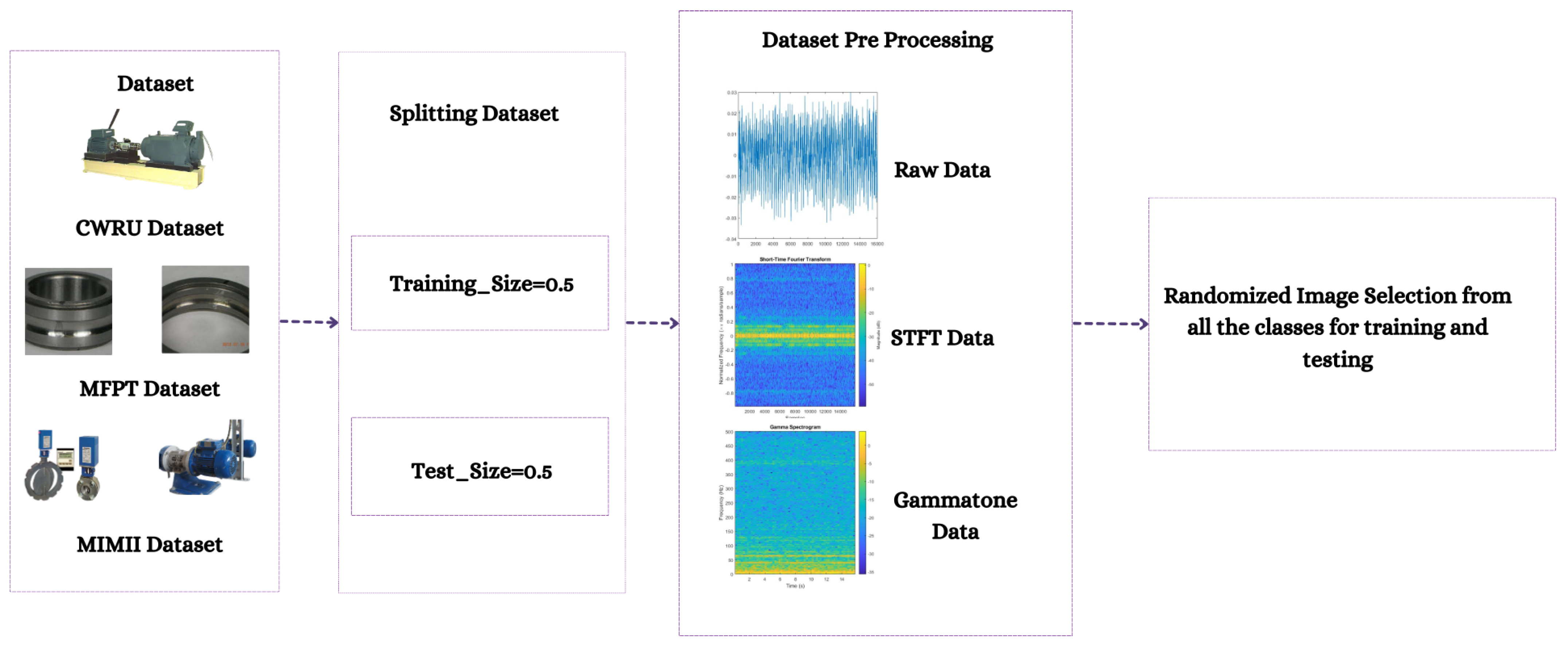
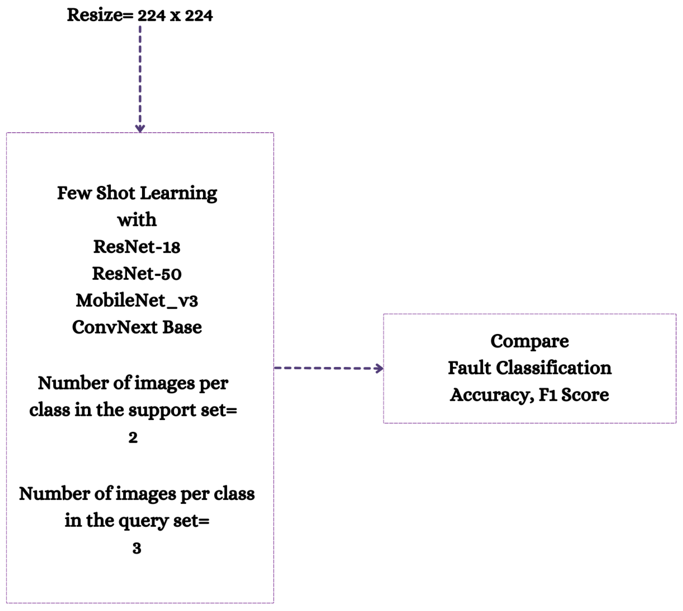
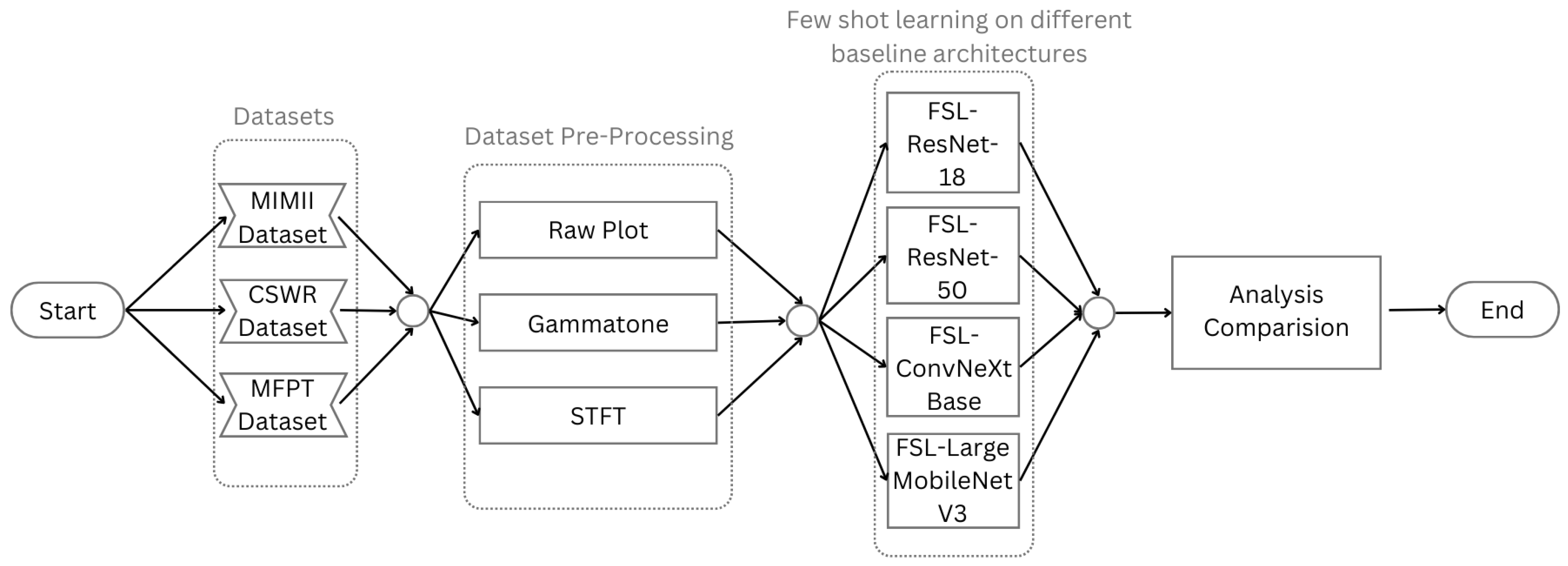
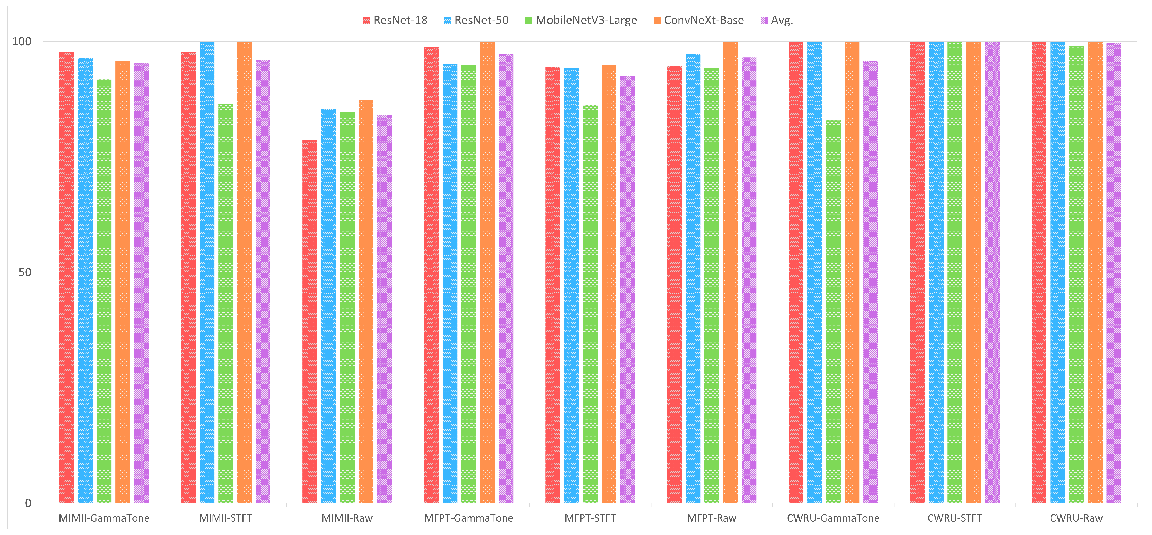
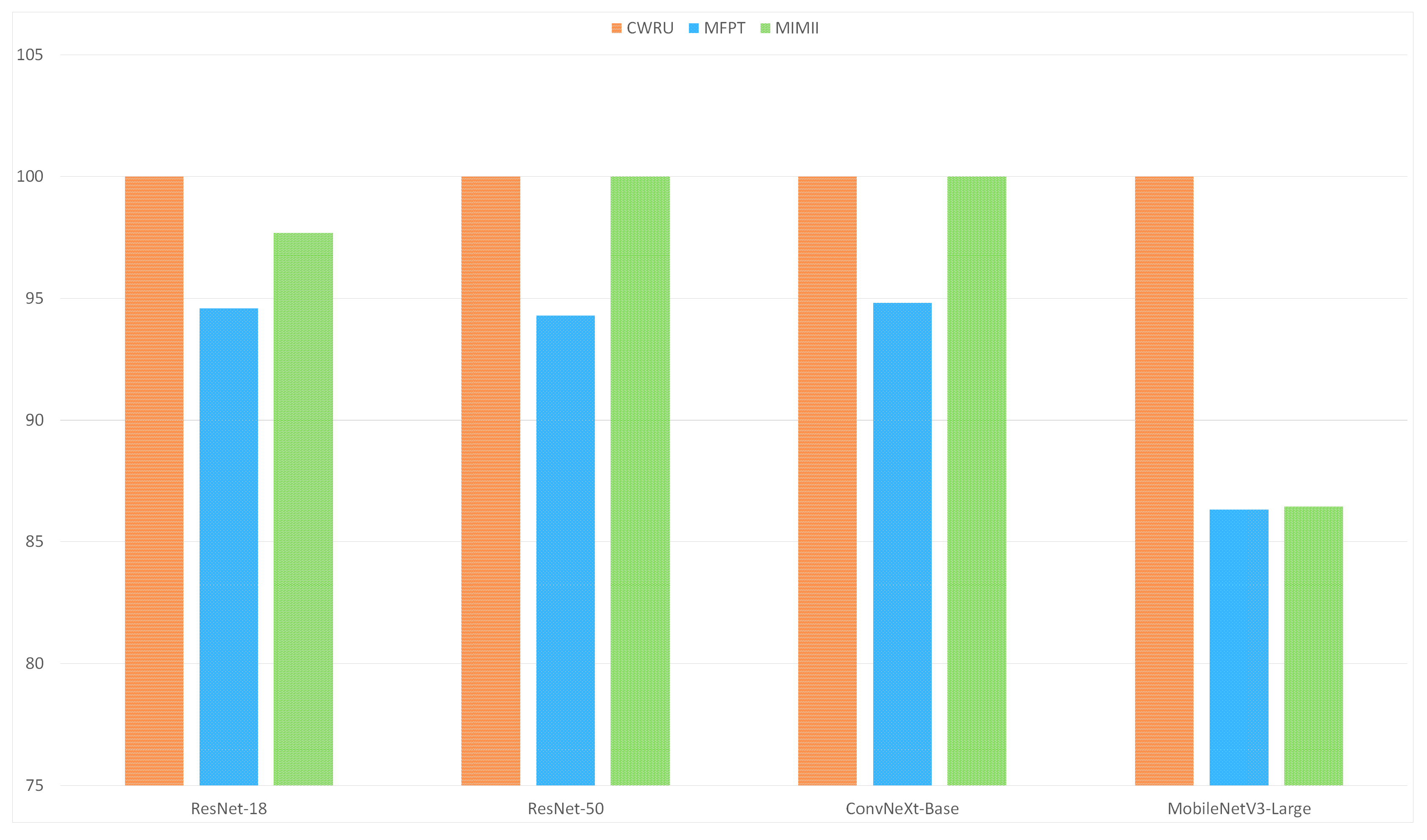
In emerging or nascent fields, as well as in professions where data collection is either difficult or costly, like industrial fault detection, tasks can be mastered using few-shot learning algorithms that generalize from limited data samples. To develop and advance few-shot learning models for machinery fault diagnosis, we followed a systematic research methodology. First, we acquired and curated a diverse repository of three datasets, including MFPT, MIMII, and CWRU. Next, we applied three data preprocessing techniques: 2D Raw Plotting, Short-Time Fourier Transform (STFT), and Gammatone Transformation. These techniques enhance feature extraction and representation, which are essential for building robust few-shot learning models. We then evaluated four architectures: ResNet-18, ResNet-50, ConvNext Base, and MobileNetV3-Large. We compared their performance under few-shot learning conditions, where labeled data is scarce. 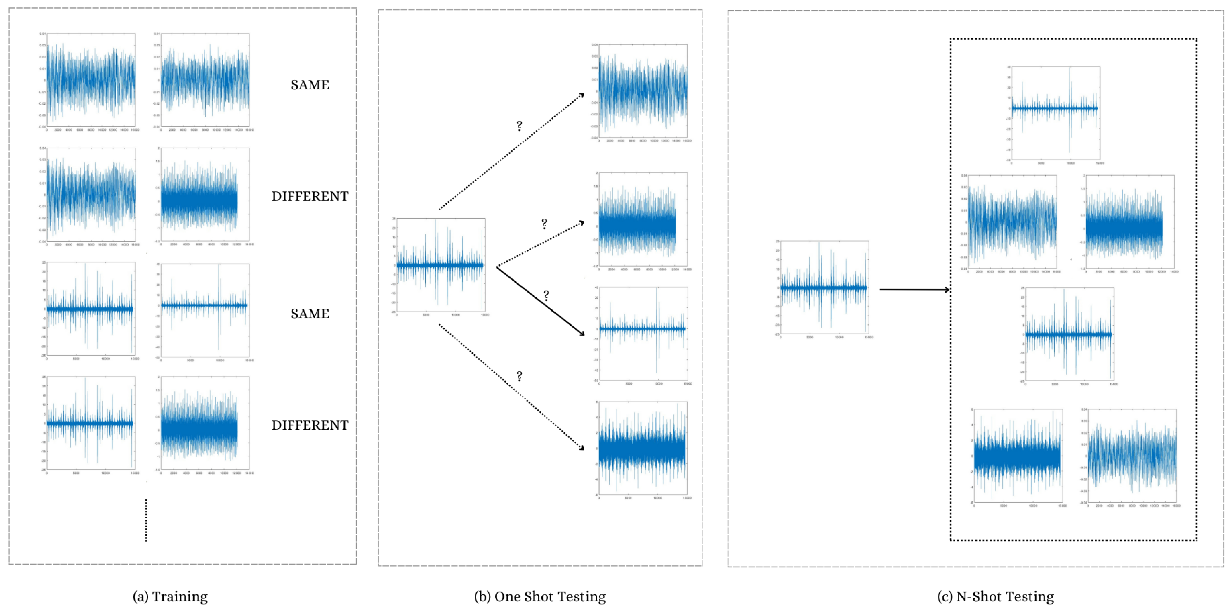In Figure 1 and Figure 2, we have shown our approach in short.

We also conducted a detailed comparative analysis of the three data preprocessing methods to understand their impact on feature enhancement. Finally, we compared and contrasted the performance of the four architectures across the curated datasets. The analysis shed light on the intricacies of few-shot learning for machinery fault diagnosis, allowing us to pinpoint the best architecture to address the challenges posed by limited labeled data.

Our research has implications for real-world applicability and potential generalization. We conclude with a summary of our findings and outline avenues for future exploration and refinement within the proposed methodology. In Figure 3, we have tried to summarize the overall methodology of our research.

3.1. Datasets

Purohit et al. introduced the MIMII dataset, a benchmark dataset for sound-based machine fault diagnosis [25]. The “MIMII Dataset” [25] is an essential tool for industrial machine inquiry and inspection since it offers a vast array of audio recordings of three different kinds of industrial machines: fans, pumps, and sliders. Our understanding of malfunction detection and assessment in industrial settings has improved because of the use of this dataset. The diversity of recording conditions is a distinguishing feature of the dataset, enhancing its realism and practicality. While the slider’s sound was recorded in a hard −6 dB setting, the audio recordings of fans and pumps were made in a controlled 0 dB environment. The value of the dataset in developing reliable and adaptable fault detection systems is enhanced by the diverse recording settings that reflect real-world situations. Each audio file in the dataset maintains a consistent sample rate of 16,000 Hz, ensuring precise recording of machine noises.

The dataset has been divided into six classes (6-way). They are Fan Abnormal, Fan Normal, Pump Abnormal, Pump Normal, Slider Abnormal, and Slider Normal.

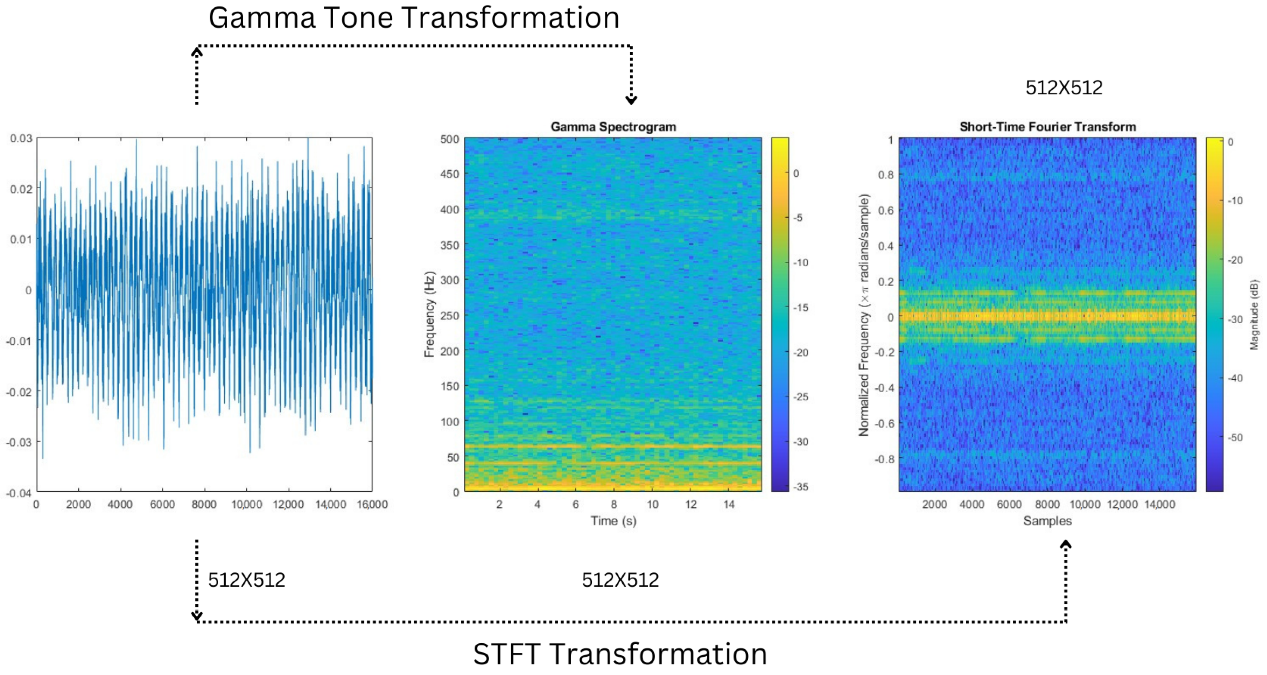
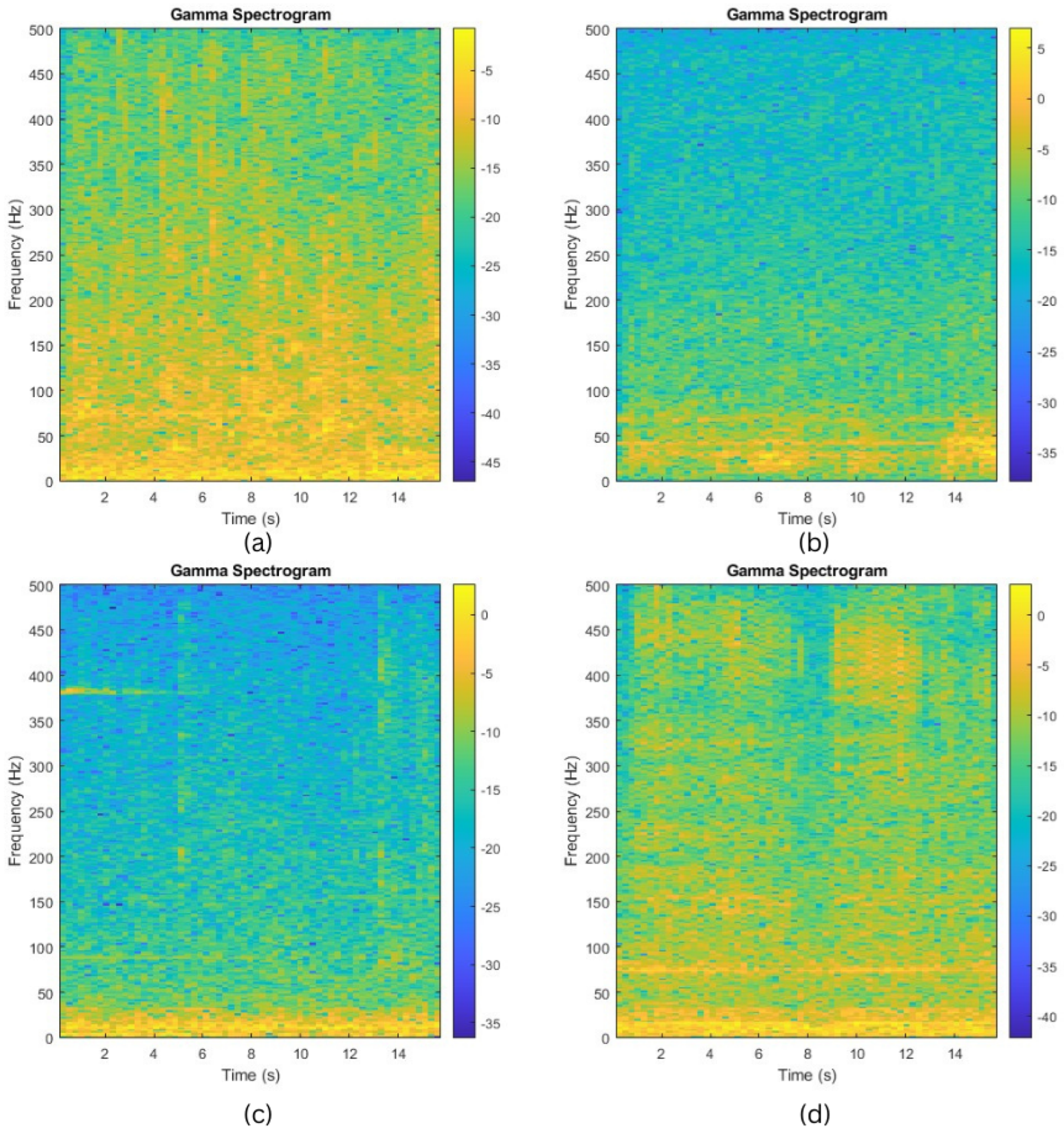
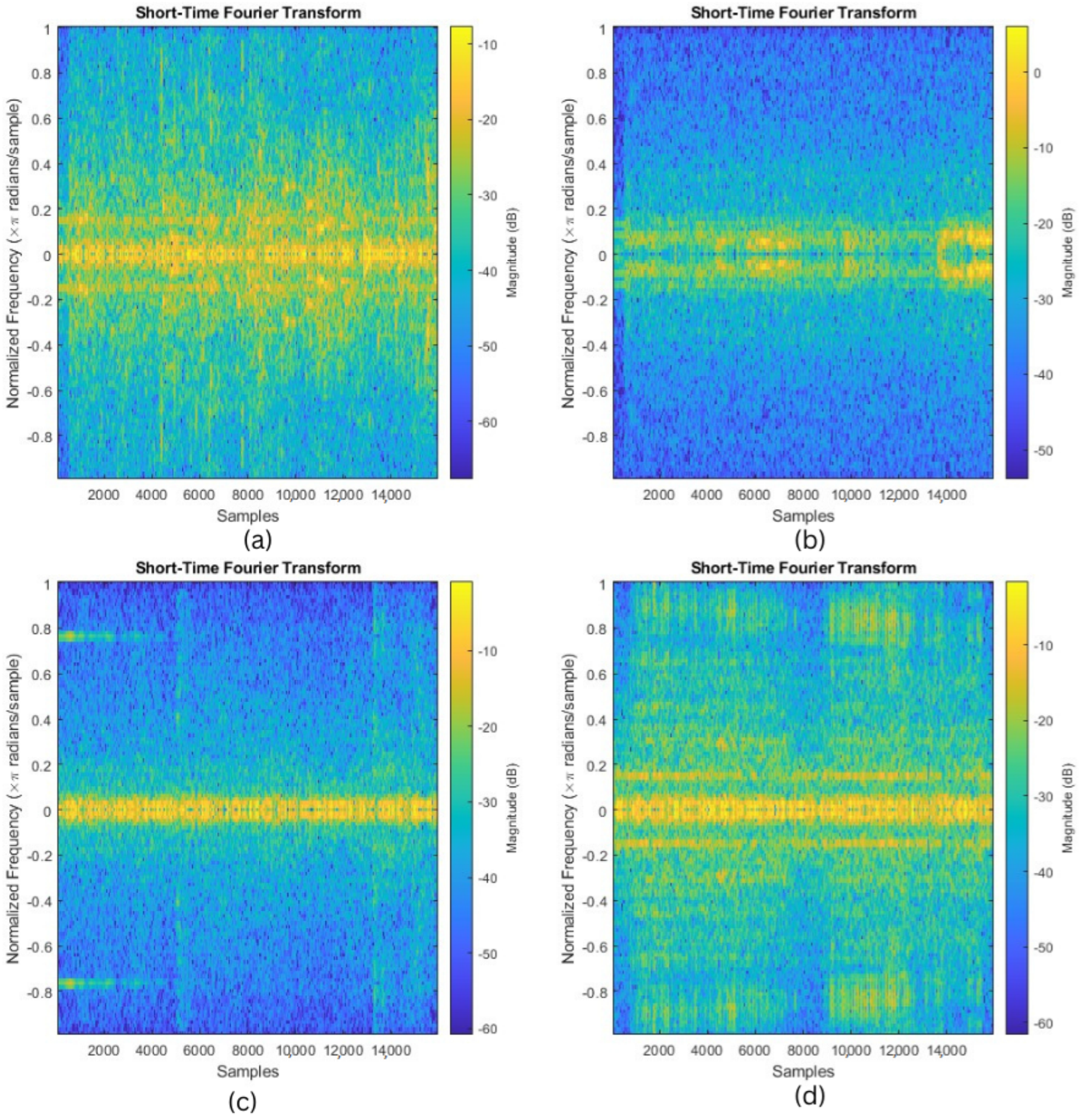
The MIMII dataset stands out for its collection of both typical and unusual machine sounds for each industrial category. This inclusion of unusual noises is important for training and assessing algorithms designed to detect errors in industrial machines. The dataset has been painstakingly divided into sub-levels to enable sophisticated analysis and feature extraction. Additionally, the dataset has been transformed using the Short-Time Fourier Transform (STFT), Gammatone treatment, and raw audio plot. These methods enable the extraction of relevant characteristics that could be crucial for differentiating between normal and pathological machine noises. The MIMII dataset offers a wide variety of real audio samples from different machines and environmental situations, making it a useful tool in the field of industrial machine study. The dataset offers a robust foundation for developing and validating innovative fault detection techniques. These methods could profoundly influence the realms of industrial maintenance and quality control due to their thorough organization, transformative analysis, and diverse sound profiles.

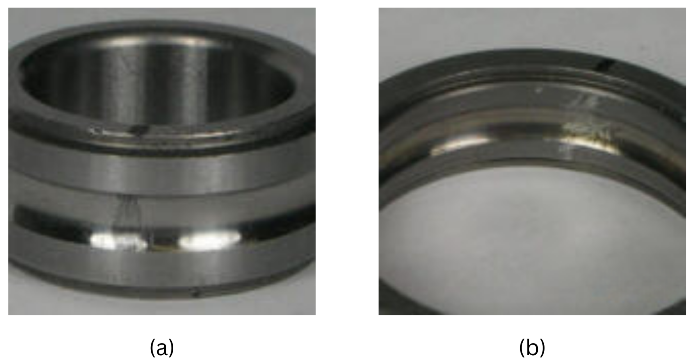
We went outside the bounds of a single dataset in our quest to improve diagnostic and prognostic algorithms for Condition-Based Maintenance (CBM), and we also made use of the “MFPT’s Dataset”. Stefaniak et al. introduced the MFPT dataset, a benchmark dataset for machine failure prediction [26]. The MFPT dataset [26] is a priceless tool created to aid in the testing and improvement of CBM systems. It was curated and compiled by Dr. Eric Bechhoefer, Chief Engineer of NRG Systems. The data that were collected from MFPT used the bearing shown in Figure 4.

To hasten the development of CBM methods and systems, this dataset serves both researchers and CBM practitioners. The dataset has been divided into four classes (4-way). They are Baseline, Inner Race Fault Varied Load, Outer Race Fault, and Outer Race Fault Varied Load. The Condition-Based Maintenance Fault Database’s main goal is to provide a wide range of rigorously recorded datasets covering various bearing and gear problems. This dataset offers a thorough assessment of diagnostic and prognosis algorithms in diverse circumstances by including scenarios of known good and faulty states. Furthermore, The MFPT dataset has a sizable bearing analysis component. The dataset contains information from a customized bearing test rig to enable an in-depth investigation of bearing behavior. In addition to nominal bearing data, outer race faults under various loads, inner race faults under varied loads, and three actual faults, this test rig covers a wide range of situations. The test rig’s bearing complies with the following requirements: Roller diameter (rd): 0.235 Pitch diameter (PD): 1.245 Number of elements (ne): 8 Contact angle (ca): 0. The dataset is structured into distinct sets of conditions, as mentioned in

Table 2. Description of Different Conditions and Parameters in the MFPT dataset.

Dataset Version	Load Levels (lbs)	Input Shaft Rate (Hz)	Sample Rate (sps)	Duration (s)
3 Baseline Conditions	270	25	97,656	6
3 Outer Race Fault Conditions	270	25	97,656	6
7 Outer Race Fault Conditions with Varied Loads	25–300	25	48,828	3
7 Inner Race Fault Conditions with Varied Loads	0–300	25	48,828	3

; each crucial for understanding different aspects of bearing behavior:

We carefully picked the dataset as well as further separated it into ten different samples to increase the depth of our study. Furthermore, we utilized the Short-Time Fourier Transform (STFT) and Gammatone Transformation, two essential signal processing methods. We were able to extract relevant characteristics from the audio data using these approaches, which may have shown patterns and differences between various circumstances that were otherwise obscured.

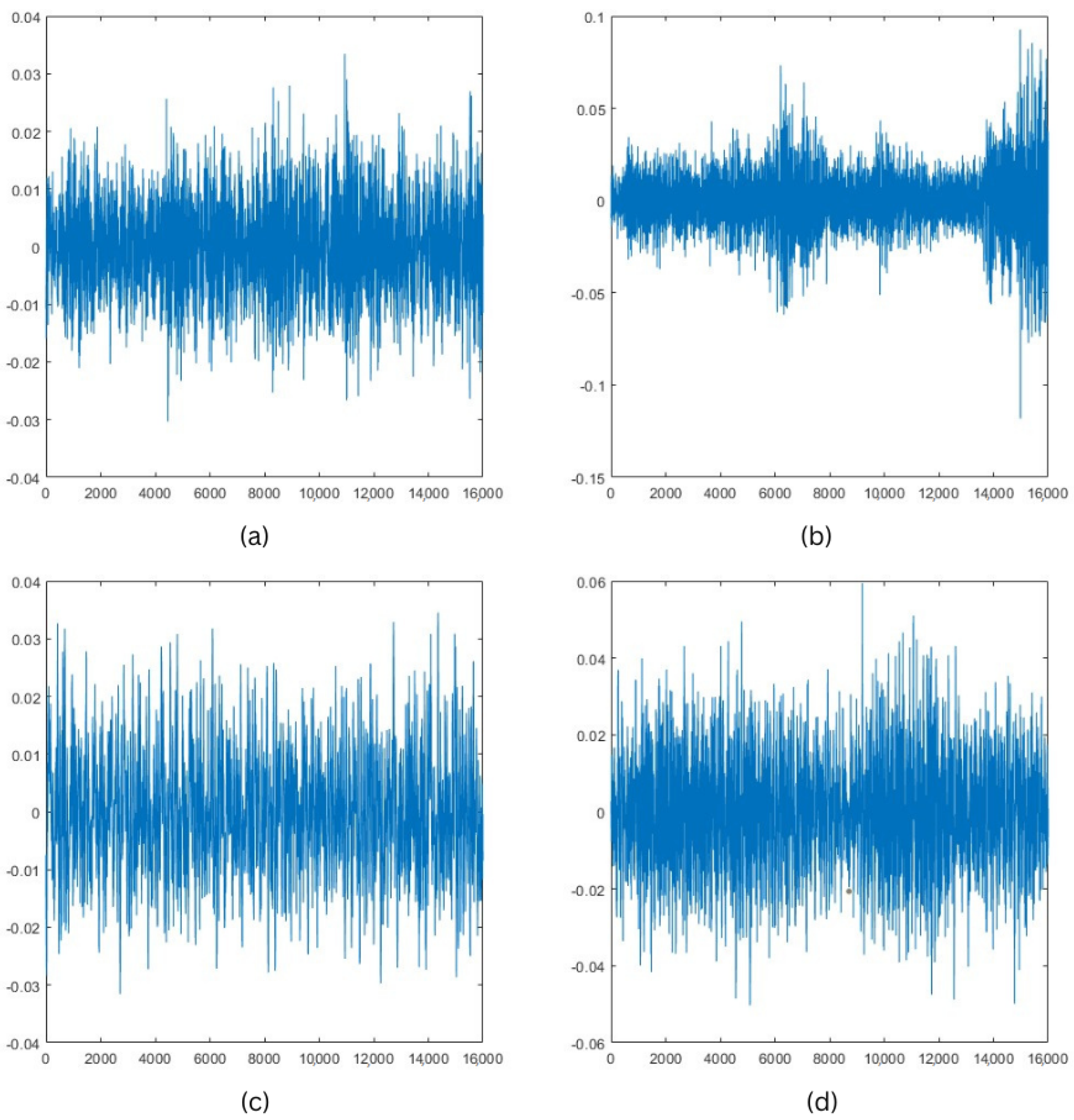
We also kept the raw signal so we could test our models. We wanted to examine the performance of our diagnostic and prognostic algorithms in their most raw form by including unprocessed data, ensuring resilience and accuracy across various settings.

In conclusion, our work involves a thorough investigation of the dataset from the MFPT, which is specially designed for developing CBM methods. We aimed to uncover insights and develop models capable of precisely diagnosing and predicting faults in industrial machinery through meticulous selection, transformative processing, and rigorous testing, ultimately assisting in the improvement and acceleration of Condition-Based Maintenance systems.

We included the priceless materials provided by the Case Western Reserve University (CWRU) Bearing Data Center [27] in the last phase of our study inquiry. This archive is a veritable gold mine of ball-bearing test data, painstakingly recording both healthy and unhealthy bearing states. The information is crucial for the field of equipment condition monitoring and provides a rare look at how motor properties and bearing health interact. A Reliance Electric motor with a 2-horsepower capacity was used in the experimental configuration. The focus was placed on acceleration data, which was captured at locations near and far from the motor bearings. These online resources’ thorough documentation of test circumstances and bearing defect status for every experiment is one of their most notable qualities. The technique of electro-discharge machining (EDM) was used to introduce defects into the motor bearings. This resulted in the introduction of a variety of flaws at the inner raceway, rolling element (ball), and outside raceway, each with a diameter ranging from 0.007 inches to 0.040 inches. The test motor was subsequently rebuilt using these defective bearings, and vibration data were methodically gathered at various motor loads, from 0 to 3 horsepower, and corresponding motor speeds, from 1797 to 1720 RPM. The dataset includes several different situations, such as those using standard bearings as well as single-point drive end and fan end faults. High sampling rates—12,000 samples per second and 48,000 samples per second for drive end-bearing experiments—were used to carefully record the data. Data from the fan end bearings was consistently gathered at a rate of 12,000 samples per second.

The dataset has been divided into five classes (5-way). They are: 12 k RPM 0.007 Diameter 0 Load Baseline; 12 k RPM 0.007 Diameter 0 Load Inner Race; 48 k RPM 0.007 Diameter 0 Load Baseline; 48 k RPM 0.007 Diameter 0 Load Inner Race, Baseline.

Each dataset file encompasses critical information, such as fan and drive-end vibration data, in addition to the motor’s rotational speed. The variable naming conventions are designed to facilitate clarity and understanding. They are DE: drive-end accelerometer data, FE: fan-end accelerometer data, BA: base accelerometer data, Time: time series data, and RPM: rotations per minute during testing. Our plan for doing this research was properly thought out. We purposefully chose particular datasets, such as the 12 k drive end, 48 k drive end, and baseline datasets. We then selected a motor speed of around 1797 RPM and a motor load of 0 horsepower for each dataset. After this, we began the meticulous process of dividing each dataset into ten distinct subgroups. These subsets went through a thorough transformation procedure that included the Short-Time Fourier Transform (STFT), analysis of the Gammatone spectrograms, and the preservation of raw data. The complex preprocessing made it possible to train and evaluate our models.

In conclusion, our interaction with the CWRU Bearing Data Center’s resources constituted an important turning point in our study. We sought to identify patterns, trends, and fault-related differences that would aid in the creation of sophisticated fault detection and prognostic algorithms by utilizing meticulously documented ball-bearing test data. We aimed to increase machine health evaluation, predictive maintenance methods, and, eventually, the reliability of industrial machinery through meticulous division, transformation, and model assessment.

3.2. Data Preprocessing

We utilized three datasets to assess our proposed model and its architecture and validate our hypothesis. Initially, we employed the MIMII dataset, a dependable resource for examining industrial machines. Second, we took advantage of the information offered by the Case Western Reserve University Bearing Data Center. Finally, we tested diagnostic and prognostic algorithms using the MFPT’s fault dataset, which is a Condition-Based Maintenance Fault Database. In Figure 5, readers can see the preprocessing overview. The WAV files and the mat files were imported into MATLAB following the selection of our datasets (which will be covered in more detail later). We utilized the Gammatone and STFT filter banks to preprocess our data.

3.2.1. Raw Plot

The plot function in MATLAB is used to produce 2D line charts of data. As shown visually in Figure 6. The plot function displays points and connects them with lines to emphasize patterns or relationships between variables, allowing for clearer data analysis. The “raw plot method” most likely refers to utilizing the plot function’s default settings without any formatting or other customization. Using extra optional arguments with the plot function allows one to alter the plot’s visual look. You may add markers to data points, alter the color and style of the lines, and more.

3.2.2. Gamma Tone Spectrogram

Gammatone filters were first introduced by Glasberg and Moore [28]. The functioning of the human auditory system served as inspiration for the creation of the gammatone filter, or spectrogram. The design aims to mimic the cochlea’s frequency-selective activity, where sound is transformed into neural impulses by the spiral-shaped component of the inner ear. Gammatone filters work particularly well for audio signal analysis, which is more in line with auditory perception in humans. The following procedures are involved in a gammatone spectrogram:

First, the audio stream is convolved using a bank of Gammatone filters in a filter bank application. These filters are made to resemble the human cochlea’s frequency response characteristics. The bank’s filters are each adjusted to a certain frequency band, allowing them to capture a separate spectral component of the signal.

Secondly, Envelope Extraction is applied. The amplitude envelope of the filtered signals is retrieved using convolution. This captures the energy distribution of the signal across various frequency bands and correlates to changes in amplitude over time.

Finally, the resultant envelopes from each filter are then used to construct a time-frequency representation, which is frequently represented as a spectrogram. This illustration, Figure 7, shows how the signal’s energy is spread over time and at different frequencies.

3.2.3. Short-Time Fourier Transform

The STFT was first introduced by Oppenheim et al. [29]. A common method for evaluating non-stationary signals, such as audio or other time-varying signals, is the short-time Fourier transform. It allows you to track variations in a signal’s frequency content over time. The STFT has a few advantages, including its versatility and its ability to localize signals in time and frequency [30]. The procedure entails dividing the signal into smaller pieces and examining the frequency content of each piece separately. Here is how STFT functions:

The window function divides the audio stream into overlapping chunks. To reduce artifacts from rapid shifts, this window function generally tapers the signal toward the segment’s edges. The Fourier transform is used to derive the frequency-domain representation of each windowed segment. This shows information about the amplitude and phase of different frequency components that are present in that segment.

A 2D representation known as a spectrogram is produced by plotting the resulting frequency-domain data across time. This illustration, Figure 8, shows how the signal’s frequencies shift over time.

3.3. Few-Shot Learning

Researchers started looking into the idea of few-shot learning in the 1980s [31], and it has since grown in significance as a means of addressing the problem of scarce data availability. With this method, we can successfully categorize data with a minimal number of instances. Let’s explore a few-shot learning’s core concepts after providing a thorough justification.

Consider teaching a model to distinguish between various items, such as cats and dogs. To aid the model’s learning, several instances of each would be required in conventional learning. However, with few-shot learning, we employ a more sophisticated strategy. This is how:

We first use pairs of data to train our model. These samples may be drawn from the same category (such as two distinct photographs of cats) or a different category (such as a cat image and a dog image). Whether the provided pairs of samples are similar or different must be taught to the model.

The model seeks to determine whether the two input samples, denoted mathematically as x and y, fall into the same category $(y=1)$ or distinct categories $(y=0)$. The chance that x and y are comparable can be produced using a function called $f(x,y)$.

Later on, we separate our data into two sets for few-shot learning: the query set and the support set. Examples of various categories are included in the support set for the model to learn from. We utilize the query set’s many categories to assess the model’s effectiveness.

Finally, one-shot k-way and N-shot k-way are the two primary testing approaches. This is what they signify:

For the one-shot k-way, by using this technique, we assess the model’s capacity to categorize new categories using just a single sample for each category. The k indicates how many various categories we are testing. Mathematically, our goal is to categorize the query sets k categories using the knowledge we’ve gained from the support set.

Lastly, for N-shot k-way, like the one-shot strategy, the N-shot k-way method tests the model using N instances from each of the k categories.

The model must generate correct classifications based on this sparse data if we have N instances for each of the k categories in the query set.

Few-shot learning has two types of representations of the task. They are: Task T, Support set $S_T$, and Query set $Q_T$. The Embedding Function is:

$$f_{\theta }:X\to {\mathbb{R}}^d$$

(1)

Additionally, the Task-Specific Embedding functions are: Embedding of support set:

$$h_i=f_{\theta }\left(x_i\right),\forall x_i\in S_T$$

(2)

Embedding of query set:

$$g_j=f_{\theta }\left(x_j\right),\forall x_j\in Q_T$$

(3)

To find the Similarity, the mentioned equation is being used (known as Cosine similarity):

$$s(h_i,g_j)=\frac{h_i·g_j}{\parallel h_i\parallel \parallel g_j\parallel }$$

(4)

Attention weights for support set examples:

$${\alpha }_i=\frac{exp\left(s(h_i,g_j)\right)}{{\sum }_{i=1}^{|S_T|}exp\left(s(h_i,g_j)\right)}$$

(5)

Weighted sum for classifying the query:

$${\widehat{y}}_j=\sum _{i=1}^{|S_T|}{\alpha }_i{h}_i$$

(6)

Lastly, the Cross-entropy loss:

$$\mathrm{Loss}=-\sum _k{y}_{j,k}log\left({\widehat{y}}_{j,k}\right)$$

(7)

In conclusion, the Few-shot learning approach shown in Figure 9 is an effective method that lets us classify data even when there are very few instances. The model is trained with pairs of samples. The data is divided into query and support sets, and the model’s ability to classify new categories is assessed using a limited sample size.

3.4. Prototypical Network

Few-shot learning supports several networks for training the model. Researchers are always looking for new approaches to overcome the difficulties presented by situations with little available data and improve the effectiveness of few-shot learning models. Ravi and Larochelle provide a comprehensive survey of few-shot learning algorithms [32]. Prototypical Networks, one of the significant techniques used, stands out because it creates category prototypes from support set samples and then uses prototype-query distance calculations to quickly and accurately classify query set samples. Similar to this, Relation Networks (RNs) excel at tasks requiring few trials by modeling relationships between pairs of inputs and emerging as potent tools for capturing complicated inter-instance correlations. Siamese Networks made up of weight-sharing twin networks, offer a convincing solution for one-shot or few-shot similarity tasks, complementing previous methods by using shared areas to learn about and quantify distances or similarities. This is especially useful in situations where learning is taking place remotely.

We have used a Prototypical Network for our research study. Prototypical networks are a simple yet effective few-shot learning algorithm [33]. Among all the available architectures for few-shot learning, we used the prototype network in this study to tackle the challenge. In few-shot learning [33,34], prototype networks generalize to new classes using a metric-based methodology. According to [1], prototypical networks outperformed other few-shot learning algorithms. To generate feature vectors and compute prototypes for recognized classes, they learn an embedding function. It is possible to estimate the similarity of classes accurately during classification by measuring the distance between query feature vectors and class prototypes. In few-shot learning, a support set of N-labeled samples

$$S=\{(x_1,y_1),\dots ,(x_n,y_n)\}$$

(8)

is supplied, where each $x_i\epsilon R^D$ is the dimensional feature vector D and each $y_i\{1...K\}\epsilon R^D$ is the label of $x_i$. $S_k$ stands for the support set’s classes. Prototype $p_k$ is calculated using an embedding function $f_{\varphi }{R}^D\to R^M$ as follows:

$$p_k=\frac{1}{\left|S_k\right|}\sum _{\left(x_i,y_i\right)\in S_k}{f}_{\varphi \left(x_i\right)}$$

(9)

The distance function d(.) is used to determine distance during classification; the likelihood that query point X belongs to class K may be represented as:

$$P_{\varphi }(y=k\mid x)=log\left(\frac{exp\left(-d\left(f_{\varphi }\left(x\right),p_k\right)\right)}{{\sum }_{k^{\prime }}exp\left(-d\left(f_{\varphi }\left(x\right),p_{k^{\prime }}\right)\right)}\right)$$

(10)

4. Experimental Result

The experimental approach and findings of our study focus on using Few-Shots Learning with four different architectures: ResNet-18, ResNet-50, ConvNeXt Base, and Large MobileNet V3. We used three types of preprocessing for our selected data. They are STFT, Gammatone Transformation, and lastly, raw plotting of the audio signals.

4.1. Experimental Setup

We used Google Colab’s free tier as our workbench, a cloud-based platform that gave us access to a Nvidia T4 GPU, 12 GB of RAM, and 15 GB of VRAM for our experiments. We employed the Python programming language, leveraging popular libraries such as NumPy, Pandas, TensorFlow, and Scikit-Learn to create machine learning models and conduct data analysis.

4.2. Evaluation Metrics

The Evaluation Metrics we have used to validate our results are given below:

• Accuracy: The classification accuracy of the model on the test dataset is the key performance metric that is assessed. It’s calculated by dividing the total number of right predictions by the total number of predictions produced by the model.

  $$\mathrm{Accuracy}=\frac{TP+TN}{TP+FN+TN+FN}$$

  (11)
• Recall: Recall refers to the percentage of total positive samples or instances that were properly anticipated to be in the positive category.

  $$\mathrm{Recall}=\frac{TP}{TP+FN}$$

  (12)
• F1-Score: The harmonic mean of a class’s precision and recall is represented by the F1-Score. It denotes the overall assessment of a model’s accuracy for that specific class.

  $$\mathrm{F1-Score}=\frac{2\times \mathrm{Precision}\times \mathrm{Recall}}{\mathrm{Precision}+\mathrm{Recall}}$$

  (13)

Among all three datasets, we implemented the following parameters for the MFPT dataset, the CWRU dataset, and the MIMII dataset; as mentioned in

Table 3. Parameters for the MFPT dataset.

Number of classes in a task (N_WAY)	4
Number of support set images per class (N_SHOT)	2
Number of query set images per class (N_QUERY)	3
Number of evaluation tasks (N_EVALUATION_TASKS)	500
Number of training episodes (N_TRAINING_EPISODES)	5000
Number of validation tasks (N_VALIDATION_TASKS)	100

,

Table 4. Parameters for the CWRU dataset.

Number of classes in a task (N_WAY)	5
Number of support set images per class (N_SHOT)	2
Number of query set images per class (N_QUERY)	3
Number of evaluation tasks (N_EVALUATION_TASKS)	500
Number of training episodes (N_TRAINING_EPISODES)	5000
Number of validation tasks (N_VALIDATION_TASKS)	100

and

Table 5. Parameters for the MIMII dataset.

Number of classes in a task (N_WAY)	6
Number of support set images per class (N_SHOT)	2
Number of query set images per class (N_QUERY)	3
Number of evaluation tasks (N_EVALUATION_TASKS)	500
Number of training episodes (N_TRAINING_EPISODES)	5000
Number of validation tasks (N_VALIDATION_TASKS)	100

.

We incorporated the Keras early stopping API into the training process. This enabled us to halt the training once the linear loss plateaued, significantly reducing both time and computational resources.

4.3. Preprocessing Comparison: STFT, Gammatone, Raw Plot for MFPT, CSWR, MIMII with ResNet-18, ResNet-50, MobileNetV3-Large, ConvNeXt-Base

We explore three preprocessing methods: Gammatone, Short-Time Fourier Transform (STFT), and raw data. We evaluate their effectiveness in the context of extracted information, lightweight architecture, and limited data availability. All the above-mentioned preprocessing techniques have been used in all three of our chosen datasets and have been diligently trained with four different models, namely Residual Neural Network-18 (ResNet-18), Residual Neural Network-50 (Resnet-50), MobileNetV3-Large, and ConvNeXt-Base.

Through rigorous experimentation, we observed that STFT consistently outperformed the other preprocessing methods, showcasing several compelling advantages: STFT’s comprehensive time-frequency representation enabled our few-shot learning models to capture both transient and spectral features inherent in fault patterns. This contributed to higher accuracy in fault classification, allowing our models to discern intricate fault signatures more effectively. Figure 10 illustrates the results based on our selected preprocessing methods run on four different models. First of all, in the MIMII dataset, STFT achieves a 96.03% accuracy on average, whereas GammaTone has an average accuracy of 95.43%, and raw data has achieved 84.04% on average. However, in the MIMII fault dataset, the average accuracy of the Raw method plummets to 84.04%, which is the lowest of all selected preprocessing methods. Finally, in the Case Western Reserve University dataset, STFT achieved 100% accuracy, leaving GammaTone behind with 95.56 and RAW behind with 99.74%.

STFT provides a detailed time-frequency representation by dividing the signal into short segments and computing the Fourier transform for each. This feature aligns well with the dynamic nature of fault patterns, enabling our few-shot learning approach to capture transient and evolving features more effectively compared with Gammatone filtering. Fault diagnosis often relies on identifying distinct spectral signatures associated with different fault types. STFT excels at retaining detailed spectral information, making it particularly valuable when diagnosing complex industrial systems with varying fault frequencies. Certain fault scenarios might involve intricate spectral variations that Gammatone filtering, due to its simplicity, might struggle to capture adequately. STFT’s ability to handle complex spectral patterns ensures that our model can accurately learn and differentiate between these nuanced fault signatures. Adaptation to Diverse Fault Types: Our chosen fault diagnosis datasets include a wide range of fault classes and operational conditions. The versatility of STFT in capturing a range of spectral features enhances the adaptability of our few-shot learning approach to the diverse fault types found in the datasets. In scenarios where the temporal localization of fault patterns is crucial, STFT’s time-frequency representation can provide insights into when and how fault signatures manifest over time. This level of detail aids in pinpointing the exact onset and evolution of faults.

Among the three preprocessing techniques, although Gammatone filtering emerges as the lightest option, STFT provides better feature extraction, which in turn increases accuracy. Given the complex nature of fault patterns, the need for spectral specificity, and the diversity of fault classes in our datasets, STFT emerged as the superior choice for our research. While Gammatone filtering offers simplicity and dimensionality reduction, STFT’s comprehensive time-frequency representation aligns more closely with the intricacies of fault diagnosis tasks and is well-suited for our lightweight architecture goals.

4.4. Architecture Comparison: ResNet-18, ResNet-50, ConvNeXt-Base, and MobileNetV3-Large with STFT for MFPT, CSWR, and MIMII

In this section, we present the results of our experiments using the Short-Time Fourier Transform (STFT) preprocessing technique with four different architectures: ResNet-18, ResNet-50, MobileNetV3-Large, and ConvNeXt-Base. We analyze the accuracy and F1-score of these models to evaluate their performance in fault diagnosis using the STFT-preprocessed data. Accuracy using STFT is illustrated in Figure 11.

The ResNet-18 model demonstrated remarkable performance with the STFT preprocessed data. Achieving an accuracy of 100% in the CWRU dataset, 94.58% in the MFPT dataset, 97.68% in the MIMII dataset, and an F1-score of 1 across all of the datasets, the confusion metric is visualized in Figure 12. ResNet-18 showcased its capacity to effectively learn and differentiate fault patterns in a few-shot learning setting. The balanced architecture of ResNet-18 combined with the enriched feature representation from STFT, contributed to its strong performance.

ResNet-50, a deeper counterpart to ResNet-18, maintained its reputation for reliable performance. With STFT-preprocessed data, it achieved an accuracy of 100% and an F1-score of 1 in the CWRU and MIMII datasets; in the MFPT dataset, it achieved 94.3% accuracy and 1 F1-score. The increased model complexity and capacity of ResNet-50 further harnessed the benefits of STFT’s comprehensive representation, resulting in enhanced fault classification accuracy. The confusion metric is shown in Figure 13.

ConvNeXt-Base, designed for efficient feature extraction, demonstrated its utility when paired with STFT-preprocessed data. It achieved an accuracy of 100% with the CWRU dataset, 94.82% with the MFPT dataset, and 100% with the MIMII dataset. It also achieved an F1-score of 1 in the CWRU and MIMII datasets and 1 with the MFPT dataset, illustrating its ability to leverage STFT’s enriched representations to identify fault patterns effectively. The confusion metric is shown in Figure 14.

MobileNetV3-Large, known for its efficiency, showcased its adaptability to STFT-preprocessed data. In the CWRU dataset, it achieved 100% accuracy and 1 as an F1-score; in the MFPT dataset, it achieved 86.32% accuracy and had an F1-score of 1; and in the MIMII dataset, it achieved 86.44% accuracy and 1 as an F1-score, highlighting its effectiveness in resource-constrained environments. The lightweight architecture of MobileNetV3-Large, combined with STFT’s detailed feature extraction, enabled accurate fault classification even with limited computational resources. The confusion metric is shown in Figure 15.

F1-Score for our research is shown below in Figure 16:

From our research results, we found that MobileNetV3-Large stands out as a lightweight model due to its innovative architectural design that prioritizes efficiency without compromising accuracy. Although it shows less accuracy than other models in the MFPT dataset, it can be enhanced with further investigation and research. Here’s why we consider MobileNetV3-Large the most suitable model for our few-shot learning approach:

A key factor contributing to the lightweight design of MobileNetV3 Large is its use of depthwise separable convolutions. Unlike traditional convolutions that process each channel with a separate kernel, depthwise separable convolutions split the convolution into two stages: depthwise and pointwise convolutions. This dramatically reduces the number of computations, leading to a lighter model. Additionally, MobileNetV3-Large employs an architecture carefully engineered for optimal performance. This design includes techniques like inverted residual blocks, which minimize the computational cost by expanding and reducing the number of channels judiciously. The network’s streamlined architecture enhances efficiency while maintaining accuracy.

Finally, MobileNetV3-Large’s parameter count is considerably lower than that of deeper architectures, for example, ResNet-50. Fewer parameters mean fewer computations during both training and inference, contributing to its lightweight character. All of the model’s parameters are summarized in

Table 6. Model Parameters.

Model	Approx. Trainable Parameters (in Millions)
MobileNetV3-Large	5
ResNet-18	11.2
ResNet-50	23.5
ConvNext-Base	14.4

.

4.5. Discussion

We have discussed the findings of our study in

Table 7. Result with the CWRU Dataset.

Preprocessing	STFT
Model Architecture	MobileNetV3 Large
Number of Training Episodes	100 (due to early stopping)
Accuracy	100.00%
Mean F1 Score	1.00

,

Table 8. Result with the MFPT Dataset.

Preprocessing	STFT
Model Architecture	MobileNetV3 Large
Number of Training Episodes	102 (due to early stopping)
Accuracy	86.32%
Mean F1 Score	1.00

and

Table 9. Result with the MIMII Dataset.

Preprocessing	STFT
Model Architecture	MobileNetV3 Large
Number of Training Episodes	161 (due to early stopping)
Accuracy	86.44%
Mean F1 Score	1.00

. These tables cover three different datasets, namely the Case Western Dataset, the MFPT dataset, and the MIMII dataset, respectively. The datasets underwent a similar preprocessing procedure that utilized the Short-Time Fourier Transform (STFT) and the Few-shot learning technique, employing a prototypical network with a MobileNetV3-Large model architecture as its backbone. The discrepancy in the number of training episodes was due to the early stopping criteria, and our primary performance metrics were the accuracy and mean F1 score. The performance on the Case Western Dataset stands out, boasting a flawless accuracy of 100.00% and an impeccable mean F1 score of 1.00. These figures reflect the model’s ability to successfully categorize faults in this dataset, demonstrating high precision and recall. Turning our attention to the MFPT dataset, the model attains an accuracy of 86.32% alongside a mean F1 score of 1.00. While the accuracy metric is marginally lower than the Case Western Dataset, the mean F1 score remains at its peak value, indicating the model’s effective discrimination of fault classes within the MFPT Dataset. Likewise, the model achieves an accuracy of 86.44% and a mean F1 score of 1.00 in the case of the MIMII dataset. Although the accuracy figure aligns with the MFPT Dataset, the model’s proficiency in distinguishing fault classes is consistently optimal. Accuracy across different datasets is shown in Figure 17.

The noteworthy mean F1 score of 1.00 across all datasets underscores the model’s excellence in precision and recall, critical attributes in fault classification tasks. While not perfect, the accuracy results signify robust classification performance on real-world fault datasets. In addition, the minor variations in the number of training episodes, owing to dataset-specific early stopping criteria, emphasize the model’s adaptability to the unique characteristics of each dataset. While the Case Western Dataset required 100 episodes, the MFPT and the MIMII datasets necessitated additional episodes (102 and 161, respectively) to achieve their respective accuracy levels.

These outcomes underscore the potential of employing the MobileNetV3 Large architecture in conjunction with STFT preprocessing for fault classification tasks. The high mean F1 scores and consistent accuracy levels across various datasets underscore the model’s versatility. These findings hold practical implications for diverse industries, including condition monitoring and predictive maintenance. A model with such robust fault classification capabilities can contribute significantly to the early detection and prevention of critical equipment failures. Training episodes taken by each dataset are shown in Figure 18.

While the results are promising, further research is imperative to evaluate the model’s performance across a broader spectrum of fault types and datasets. Moreover, investigating alternative preprocessing techniques and model architectures may yield valuable insights for potential enhancements. Different Few-shot learning algorithms could also be explored to solidify the findings.

In conclusion, our study suggests that the combination of MobileNetV3-Large and STFT preprocessing encompassed within prototypical networks and Few-shot learning holds significant promise for machinery fault classification. The elevated mean F1 scores and commendable accuracy levels confirm the model’s suitability for practical applications in real-world scenarios.

5. Conclusions

This study highlights the promise of few-shot learning combined with the MobileNet architecture for equipment failure diagnostics in its conclusion. A model that performed well across many datasets was produced by carefully selecting architecture, preprocessing methods, and hyperparameters. Our study contributes to the expanding body of knowledge at the interface between machine learning and industrial applications and offers insightful suggestions for improving fault detection and preventative maintenance techniques. While working with the few-shot learning model, we found that FSL may have trouble dealing with complicated problems that require in-depth comprehension and efficient information transfer across various industrial contexts. These problems necessitate resource-intensive fine-tuning and domain knowledge for maximum performance. Therefore, for our future work, we aim to overcome this limitation of the model. We discovered that specialized data augmentation, blending with conventional techniques, semi-supervised learning, multimodal approaches, and domain adaptability should all be investigated to overcome these limitations.

References

1. Smith, J.D.; Johnson, A.B. Recent Advances in Intelligent Fault Diagnosis: A Comprehensive Review. J. Ind. Eng. 2020, 15, 678–698. [Google Scholar]
2. Zhang, H.; Zhao, Y. A Review on Sensor Fault Detection and Diagnosis Methods. IEEE Access 2018, 6, 6472–6484. [Google Scholar]
3. LeCun, Y.; Bengio, Y.; Hinton, G. Deep learning. Nature 2015, 521, 436–444. [Google Scholar] [CrossRef] [PubMed]
4. Pan, S.J.; Yang, Q. A survey on transfer learning. IEEE Trans. Knowl. Data Eng. 2010, 22, 1345–1359. [Google Scholar] [CrossRef]
5. Analytics Vidhya. 10 May 2021. An Introduction to Few-shot learning. Available online: https://www.analyticsvidhya.com/blog/2021/05/an-introduction-to-few-shot-learning/ (accessed on 23 August 2023).
6. Han, T.; Liu, C.; Yang, W.; Jiang, D. Deep transfer network with joint distribution adaptation: A new intelligent fault diagnosis framework for industry application. ISA Trans. 2020, 97, 269–281. [Google Scholar] [CrossRef]
7. Qi, G.; Yao, L.; Uzunov, A.V. Fault detection and localization in distributed systems using recurrent convolutional neural networks. In Proceedings of the Advanced Data Mining and Applications: 13th International Conference, ADMA 2017, Singapore, 5–6 November 2017; Proceedings 13. Springer International Publishing: Berlin/Heidelberg, Germany, 2017; pp. 33–48. [Google Scholar]
8. Yin, Z.; Hou, J. Recent advances on SVM based fault diagnosis and process monitoring in complicated industrial processes. Neurocomputing 2016, 174, 643–650. [Google Scholar] [CrossRef]
9. Uddin, J.; Kang, M.; Nguyen, D.V.; Kim, J.M. Reliable fault classification of induction motors using texture feature extraction and a multiclass support vector machine. Math. Probl. Eng. 2014, 2014, 814593. [Google Scholar] [CrossRef]
10. Jian, C.; Yang, K.; Ao, Y. Industrial fault diagnosis based on active learning and semi-supervised learning using small training set. Eng. Appl. Artif. Intell. 2021, 104, 104365. [Google Scholar] [CrossRef]
11. Wang, H.; Wang, J.; Zhao, Y.; Liu, Q.; Liu, M.; Shen, W. Few-shot learning for fault diagnosis with a dual graph neural network. IEEE Trans. Ind. Inform. 2022, 19, 1559–1568. [Google Scholar] [CrossRef]
12. Zabin, M.; Choi, H.J.; Uddin, J. Hybrid deep transfer learning architecture for industrial fault diagnosis using Hilbert transform and DCNN–LSTM. J. Supercomput. 2023, 79, 5181–5200. [Google Scholar] [CrossRef]
13. Liu, H.; Yu, C.; Yu, C. A new hybrid model based on secondary decomposition, reinforcement learning and SRU network for wind turbine gearbox oil temperature forecasting. Measurement 2021, 178, 109347. [Google Scholar] [CrossRef]
14. Yan, G.; Yu, C.; Bai, Y. A new hybrid ensemble deep learning model for train axle temperature short term forecasting. Machines 2021, 9, 312. [Google Scholar] [CrossRef]
15. Kramer, M.A.; Palowitch, B.L., Jr. A rule-based approach to fault diagnosis using the signed directed graph. AIChE J. 1987, 33, 1067–1078. [Google Scholar] [CrossRef]
16. Xu, Y.; Li, Z.; Wang, S.; Li, W.; Sarkodie-Gyan, T.; Feng, S. A hybrid deep-learning model for fault diagnosis of rolling bearings. Measurement 2021, 169, 108502. [Google Scholar] [CrossRef]
17. Vinyals, O.; Blundell, C.; Lillicrap, T.; Wierstra, D. Matching networks for one shot learning. Adv. Neural Inf. Process. Syst. 2016, 29, 3607–3617. [Google Scholar]
18. Wang, Y.; Yao, Q.; Kwok, J.; Ni, L. Generalizing from a Few Examples: A Survey on Few-shot Learning. ACM Comput. Surv. 2020, 53, 1–34. [Google Scholar] [CrossRef]
19. Gharoun, H.; Momenifar, F.; Chen, F.; Gandomi, A.H. Meta-learning approaches for few-shot learning: A survey of recent advances. arXiv 2023, arXiv:2303.07502. [Google Scholar]
20. Brown, T.; Mann, B.; Ryder, N.; Subbiah, M.; Kaplan, J.D.; Dhariwal, P.; Neelakantan, A.; Shyam, P.; Sastry, G.; Askell, A.; et al. Language models are few-shot learners. Adv. Neural Inf. Process. Syst. 2020, 33, 1877–1901. [Google Scholar]
21. Gao, T.; Fisch, A.; Chen, D. Making pre-trained language models better few-shot learners. arXiv 2020, arXiv:2012.15723. [Google Scholar]
22. Dhillon, G.S.; Chaudhari, P.; Ravichandran, A.; Soatto, S. A Baseline for Few-Shot Image Classification. arXiv 2019, arXiv:1909.02729. [Google Scholar]
23. Ravi, S.; Larochelle, H. Optimization as a model for few-shot learning. In Proceedings of the International Conference on Learning Representations, San Juan, PR, USA, 2–4 May 2016. [Google Scholar]
24. Sun, Q.; Liu, Y.; Chua, T.S.; Schiele, B. Meta-transfer learning for few-shot learning. In Proceedings of the IEEE/CVF Conference on Computer Vision and Pattern Recognition, Long Beach, CA, USA, 16–20 June 2019; pp. 403–412. [Google Scholar]
25. Purohit, H.; Tanabe, R.; Ichige, K.; Endo, T.; Nikaido, Y.; Suefusa, K.; Kawaguchi, Y. MIMII: A benchmark dataset for sound-based machine fault diagnosis. arXiv 2019, arXiv:1909.09347. [Google Scholar]
26. Stefaniak, M.; Kaczmarczyk, M.; Kasprzak, M. MFPT: A benchmark dataset for machine failure prediction. Sensors 2023, 23, 4469. [Google Scholar]
27. Case Western Reserve University Bearing Data Center. Download a Data File. Available online: https://engineering.case.edu/bearingdatacenter/download-data-file (accessed on 23 August 2023).
28. Glasberg, B.R.; Moore, B.C.J. Auditory filter shapes derived from the cochlea. Hear. Res. 1990, 47, 103–138. [Google Scholar] [CrossRef] [PubMed]
29. Oppenheim, A.V.; Schafer, R.W.; Buck, J.R. The theory of linear prediction and optimum filters. IEEE Trans. Acoust. Speech Signal Process. 1969, 17, 294–309. [Google Scholar]
30. Chen, Z.; Li, J. Short-time Fourier transform: A versatile tool for time-frequency analysis. Signal Process. 2019, 159, 13–19. [Google Scholar] [CrossRef]
31. Ravi, S.; Larochelle, H.; Courville, A.; Bengio, Y. Learning to learn with few shot examples. arXiv 2016, arXiv:1604.00257. [Google Scholar]
32. Ravi, S.; Larochelle, H. Few-shot learning: A survey of methods and applications. arXiv 2019, arXiv:1904.04210. [Google Scholar]
33. Snell, J.; Swersky, K.; Zemel, R.S. Prototypical networks for few-shot learning. arXiv 2017, arXiv:1703.05175, 225–250. [Google Scholar]
34. Vinyals, O.; Blundell, C.; Lillicrap, T.P.; Kavukcuoglu, K.; Rusu, A.A. Matching networks for few-shot learning. arXiv 2016, arXiv:1606.04088. [Google Scholar]
Figure 1. Workflow of the proposed methodology. Data Collection.
Vibration 06 00059 g001
Figure 2. Few Shot Learning Approach.
Vibration 06 00059 g002
Figure 3. Summary proposed methodology.
Vibration 06 00059 g003
Figure 4. Two bearings that were used to record the MFPT data set. (a) Innerrace Bearing. (b) Outerrace Bearing.
Vibration 06 00059 g004
Figure 5. Data Preprocessing.
Vibration 06 00059 g005
Figure 6. A sample of Raw data (a) Pump Normal at 0 dB. (b) Pump Abnormal at 0 dB. (c) Slider Normal at −6 dB. (d) Slider Abnormal at −6 dB.
Vibration 06 00059 g006
Figure 7. A sample of Gamma tone spectrum (a) Pump Normal at 0dB. (b) Pump Abnormal at 0 dB. (c) Slider Normal at −6 dB. (d) Slider Abnormal at −6 dB.
Vibration 06 00059 g007
Figure 8. A sample of STFT data (a) Pump Normal at 0 dB. (b) Pump Abnormal at 0 dB. (c) Slider Normal at −6 dB. (d) Slider Abnormal at −6 dB.
Vibration 06 00059 g008
Figure 9. Few Shot Training and Testing Strategy (a) Training. (b) One Shot Testing. (c) N Shot Testing.
Vibration 06 00059 g009
Figure 10. Identification of accuracy % of the models with different preprocessing methods.
Vibration 06 00059 g010
Figure 11. Accuracy % of different models with the data sets preprocessed with STFT.
Vibration 06 00059 g011
Figure 12. Confusion Matrix for ResNet-18 Architecture: MFPT Dataset, CSWR Dataset and MIMII Dataset using STFT preprocessing.
Vibration 06 00059 g012
Figure 13. Confusion Matrix for ResNet-50 Architecture: MFPT Dataset, CSWR Dataset and MIMII Dataset using STFT preprocessing.
Vibration 06 00059 g013
Figure 14. Confusion Matrix for ConvNeXt-Base Architecture: MFPT Dataset, CSWR Dataset and MIMII Dataset using STFT preprocessing.
Vibration 06 00059 g014
Figure 15. Confusion Matrix for MobileNetV3-Large Architecture: MFPT Dataset, CSWR Dataset and MIMII Dataset using STFT preprocessing.
Vibration 06 00059 g015
Figure 16. F1-score of the models in our tested datasets.
Vibration 06 00059 g016
Figure 17. Accuracy across different dataset.
Vibration 06 00059 g017
Figure 18. Training Episode across different datasets.
Vibration 06 00059 g018