
Vibration Transmission across Seismically Damaged Beam-to-Column Junctions of Reinforced Concrete Using Statistical Energy Analysis

1
Institute for Risk and Uncertainty, University of Liverpool, Liverpool L69 7ZF, UK
2
Acoustics Research Unit, School of Architecture, University of Liverpool, Liverpool L69 7ZN, UK
*
Authors to whom correspondence should be addressed.
Vibration 2023, 6(1), 149-164; https://doi.org/10.3390/vibration6010011
Submission received: 25 October 2022
/
Revised: 21 January 2023
/
Accepted: 31 January 2023
/
Published: 2 February 2023
(This article belongs to the Special Issue Feature Papers in Vibration)
Abstract
:To detect human survivors trapped in buildings after earthquakes by using structure-borne sound it is necessary to have knowledge of vibration transmission in collapsed and fragmented reinforced-concrete buildings. In this paper, statistical energy analysis (SEA) is considered for modelling vibration transmission in seismically damaged, reinforced concrete, beam-to-column junctions where the connection between the beam and the column is made only via the steel reinforcement. An ensemble of 30 randomly damaged beam-to-column junctions was generated using a Monte Carlo simulation with FEM. Experimental SEA (ESEA) is then considered with two or three subsystems to determine the coupling loss factors (CLFs) between the beam and the column with either bending modes or the combination of all mode types. It is shown that bending modes dominate the dynamic response and that the uncertainty of predicting the CLFs using FEM with ESEA is sufficiently low that it should be feasible to estimate the coupling even when the exact angle between the beam and the column is unknown. In addition, the use of two rather than three subsystems for the junction significantly decreases the number of negative coupling loss factors with ESEA. An initial analysis of the results in this paper was presented at the 50th International Congress and Exposition on Noise Control Engineering.
1. Introduction
Every few years, an earthquake of high magnitude occurs in the world, resulting in collapsed structures with people trapped inside them. When victims are trapped inside a collapsed building, the challenge is to detect and locate survivors within a period that will allow them to be rescued. Although most documented live rescues are accomplished within the first six days of the entrapment [1], an uninjured healthy adult with a supply of fresh air has a higher probability of survival if the rescue occurs within 72 h [1,2]. The variables that affect the survivability are the cause of the structural collapse and the speed and sophistication of available urban search and rescue (USAR) capabilities [3]. Airborne sound from survivors tends to be highly attenuated by layers of rubble and requires the existence of air paths for propagation to the surface. For this reason, there is greater potential to detect physical movement or signals from survivors by measuring structure-borne sound near the surface (i.e., seismic research method [4]). To assess the potential to predict vibration transmission in collapsed and fragmented reinforced-concrete buildings, this work builds on previous research on the structural dynamics of stacked concrete beams with surface contacts [5]. This has the potential to inform decisions about the possibility to detect trapped human survivors using structure-borne sound.
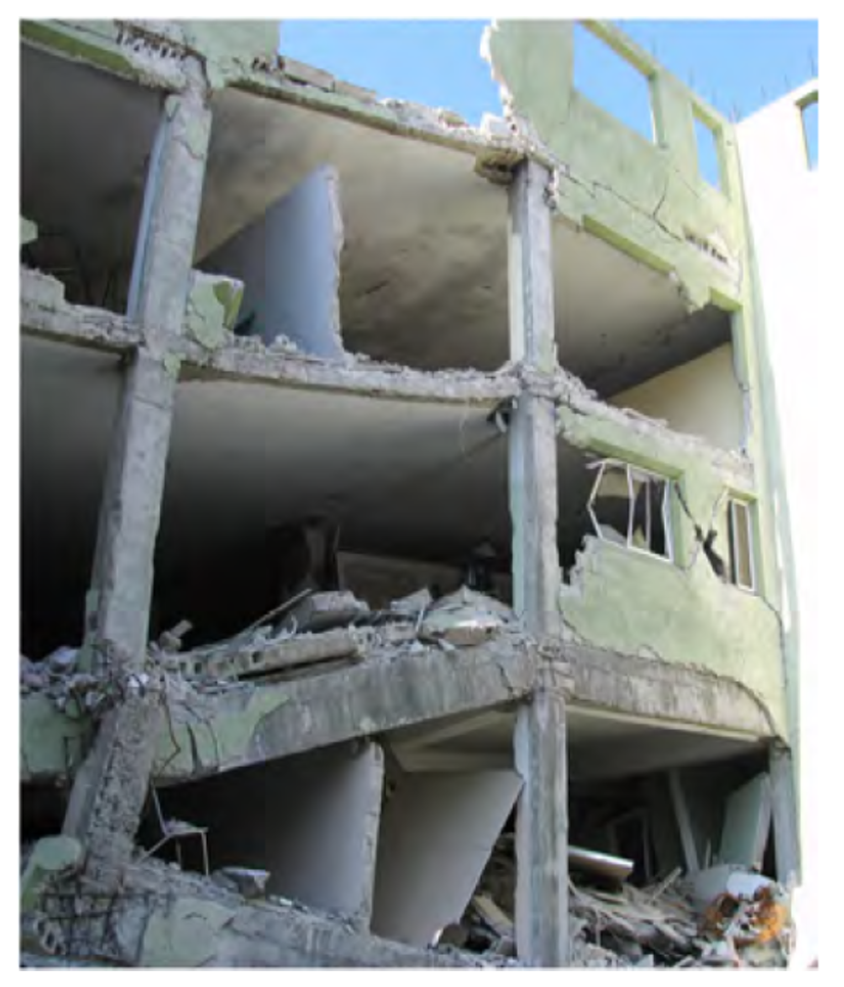
A lean-to-collapse (see Figure 1) is one of the most frequent types of collapse patterns in heavy floor structures such as reinforced concrete buildings [6]. It occurs when one end of a floor is supported by a fragmented structural member or debris and the opposite end remains connected to a column [7]. The angle between the anchored floor and the column is usually between 45° and 55° [8] and the only connection is made via the yielded steel reinforcement [9].
To predict vibration transmission across fractured beam-to-column junctions, it is proposed that statistical energy analysis (SEA) [10] could be used because it can account for the inherent uncertainty in describing modal features of component parts of a structure. Beams and columns act as SEA subsystems which store modal energy and the coupling parameter that describes energy flow between subsystems is the coupling loss factor (CLF). For complex junctions in heavyweight buildings, experimental statistical energy analysis (ESEA) has previously been combined with finite element methods (FEM) to determine these CLFs [11,12], and this approach could potentially be used for fragmented structures.
SEA models of rigid T-junctions in heavyweight buildings usually assume that each of the three beams/plates can be represented by a single subsystem for each wave type [13]. However, the authors are not aware of any work on modelling vibration transmission across damaged T-junctions where the connection between the beam and the column is made only via the yielded steel reinforcement. This paper investigates whether these junctions could be modelled using three subsystems or whether the existence of the fracture causes the parts of the column above and below the beam to act as a single subsystem. It also investigates whether it is possible to only consider bending waves or whether two or more types of wave motion need to be considered simultaneously (e.g., bending and torsional waves). A FEM model of an undamaged rigid T-junction is validated against the wave theory in terms of CLFs that only consider bending wave motion. A concrete discontinuity is then introduced at the connection of the beam with the column and numerical experiments are carried out with FEM to create an ensemble of beam-to-column junctions for a Monte Carlo simulation which will allow use of ESEA to determine the CLFs. An assessment is made on whether the number of subsystems affects the validity and accuracy of FEM ESEA and whether it is possible to only consider one type of wave motion (e.g., bending waves) or whether two or more types of wave motion could be considered simultaneously (e.g., bending and torsional waves). Consideration of ESEA with multiple wave types is necessary because in a collapsed structure it is not known whether one or more wave types will be excited at the damaged beam-to-column connection.
Figure 1.
Lean-to-collapse pattern in reinforced concrete building [14].
Figure 1.
Lean-to-collapse pattern in reinforced concrete building [14].

2. Materials and Methods
2.1. Beam-to-Column Junctions
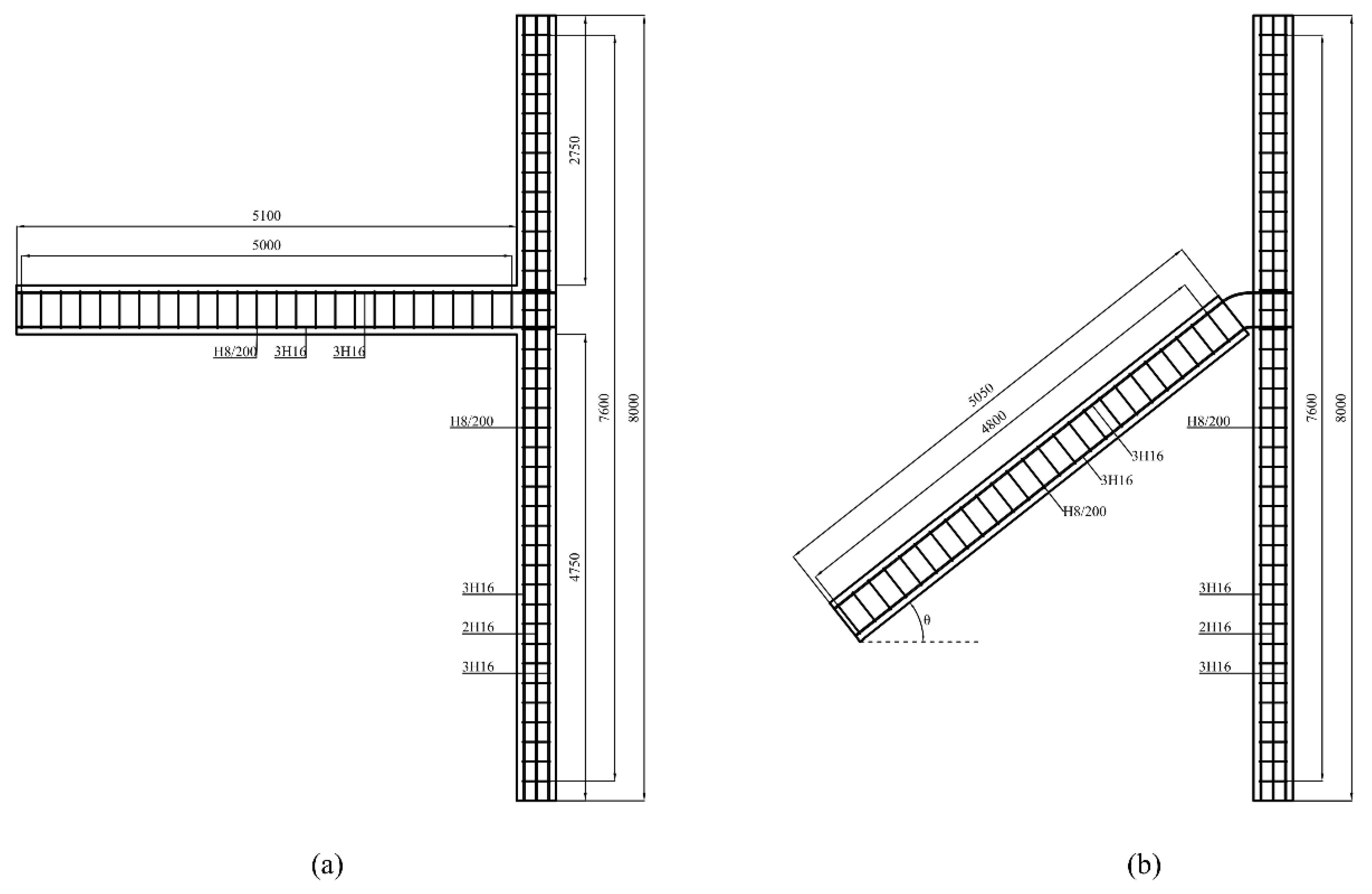
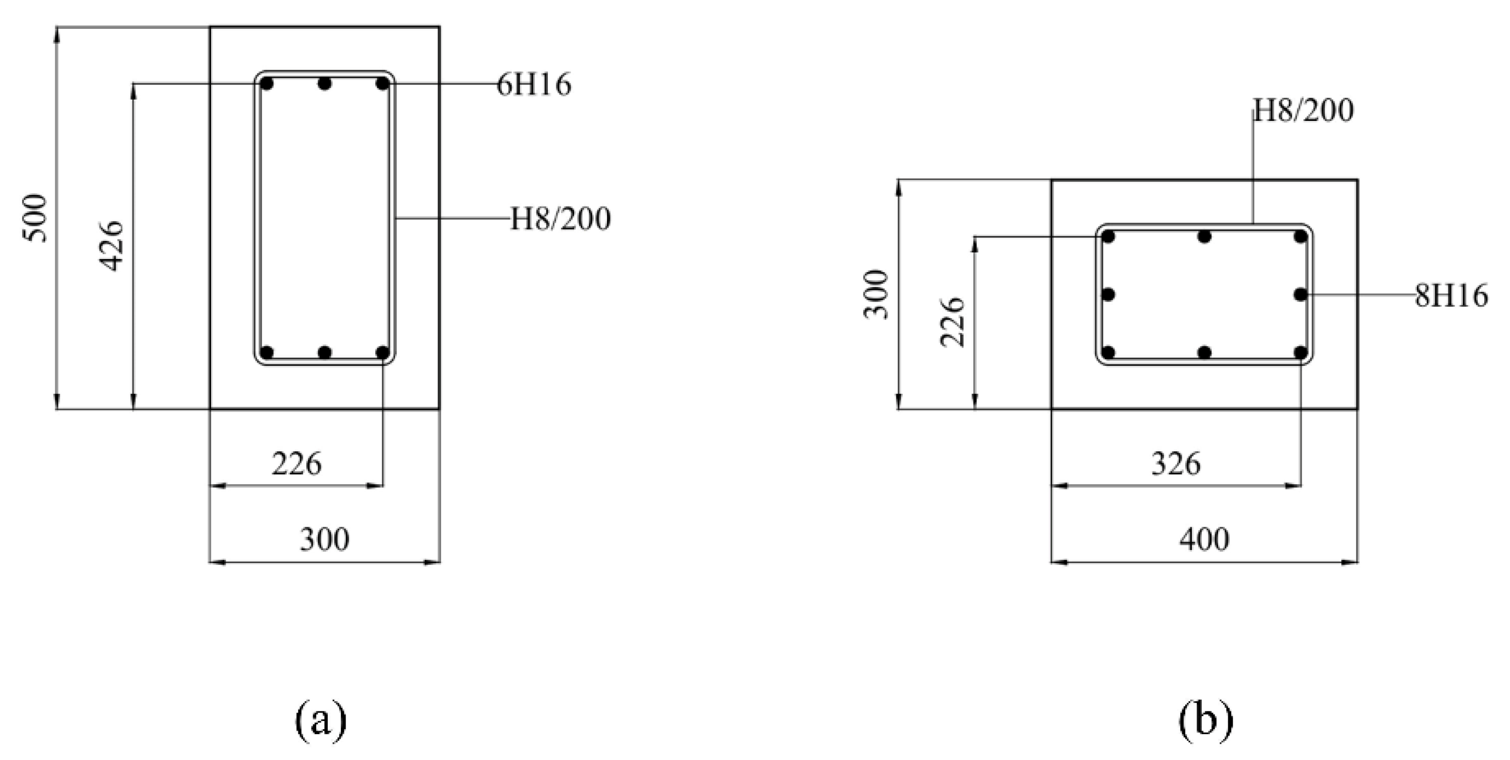
The junctions consist of a reinforced concrete beam (5.1 m length, 0.3 m width and 0.5 m depth) and a reinforced concrete column (8.0 m length, 0.4 m width and 0.3 m depth)—see Figure 2. The beam and the column are reinforced with six or eight longitudinal steel bars of 16 mm diameter, respectively, and the transverse reinforcement consists of 8 mm diameter stirrups placed at 200 mm centres along the beams (see Figure 3). Two types of junctions were considered as shown in Figure 1: (a) undamaged (rigid junction) and (b) damaged with a concrete discontinuity of 50 mm between the beam and the column where the beam is rotated by the angle, θ and connected to the column via the longitudinal steel reinforcement.
2.2. Finite Element Modelling
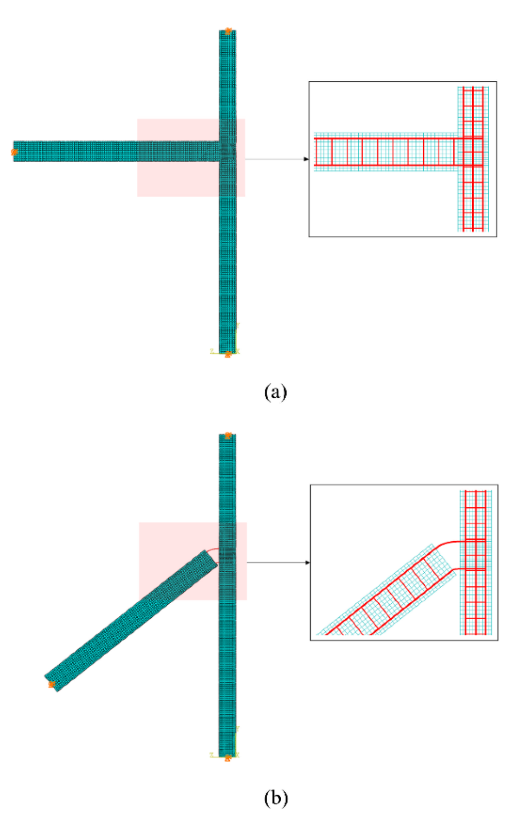
FEM modelling was carried out using Abaqus v6.14 [15]. The solid element C3D20R (20 nodes) and the beam element B32 (3 nodes) were used to model the concrete and the steel bars, respectively (see Figure 4). This approach for modelling the steel bars in reinforced concrete members with and without discontinuities was validated in previous work by the authors [5,16]. The mesh density fulfils the requirement to have at least six elements per wavelength for structural dynamics problems [17]. Tie constraints were used for modelling the rigid connection between the beam and the column in the undamaged junction. Both the beam and the column were assumed to be simply supported at the ends.
Mode-based steady-state dynamic analysis was used to calculate the dynamic response of the junctions up to 3200 Hz considering either the out-of-plane bending modes or the combination of all modes. At the nodes along the length of each beam or column, the type of excitation was ‘rain-on-the-roof’ which comprises of unity forces with random phase. The critical damping, ζ, was set to 0.05. Table 1 shows the physical and mechanical properties of the materials used in the FEM model [5].
2.3. Monte Carlo Simulation for ESEA
SEA predicts the mean response of an ensemble of similar systems; therefore, a Monte Carlo simulation using FEM and ESEA is used to calculate average responses and quantify the uncertainty; this approach is referred to in this paper as ‘FEM ESEA’. The technique is based on random number generation to determine each variable based on a chosen statistical distribution [18]. A sample of 30 damaged beam-to-column junctions was created using a Monte Carlo simulation with FEM. The angle between the beam and the column in a damaged junction is typically between 45° and 55° [8]. However, in this paper, the angle, θ, (see Figure 2b) was sampled from a uniform distribution θ~U(−80,80) to include more extreme angles in the ensemble and assess whether there was a significant variation with angle.
2.4. Experimental Statistical Energy Analysis
As with SEA, ESEA determines the average response in a frequency band. In this paper these frequency bands are chosen to have a bandwidth of 200 Hz so that each subsystem has at least one mode in each frequency band. The standard approach to ESEA relies on the power injection method where the coupling loss factors are determined by the inversion of the power balance equations [19]. This requires knowledge of the power inputs and the subsystem energies.
Woodhouse [20] noted that any errors in quantifying the energies could lead to problems with the generation of negative CLFs. However, the use of FEM rather than physical experiments with ESEA potentially avoids some errors with sampling because the entire mesh of finite element responses is used over a subsystem. ESEA has previously been used with FEM for coupled heavyweight plates (L- and T-junctions) that have low modal overlap and low modal density [12]. For L-junctions there were no negative CLFs and this finding supported the hypothesis of Woodhouse [20] that SEA and ESEA is always applicable to two coupled subsystems. However, with T-junctions, there were negative CLFs for transmission across the straight section of a T-junction for 27% of the ensemble in some frequency bands. The risk of ESEA producing negative CLFs tends to increase when there are three or more subsystems [20]. To try and address this issue, optimisation processes have been developed to increase the chances of determining a loss factor matrix that could form the basis of a suitable SEA model, e.g., see [21,22,23]. However, Lalor [24] noted potential problems with optimization in that the ability to significantly alter a CLF also implied that optimized values might not be reliable; hence, an alternative matrix solution was proposed to try and overcome the problem of ill-conditioned ESEA matrices. When several subsystems are assigned in general forms of ESEA, rules have been developed to try and avoid negative CLFs; these have been validated with six-subsystem ESEA for coupled air volumes [25]. However, buildings rarely have more than four subsystems connected at a junction and for the damaged T-junction it is feasible, and reasonable (because there is no significant impedance mismatch at the junction), to consider the entire column as a single subsystem. This gives the potential to represent the damaged T-junction by two subsystems and potentially avoid negative CLFs.
The ESEA matrix solution for two and three subsystems is given by [18]
where ηij is the coupling loss factor from subsystem i to j, ηii is the internal loss factor for subsystem i and Eij is the energy of subsystem i when the power is input into subsystem j, Win(i) is the power injected into subsystem i, and ω is the angular frequency.
The energy associated with each subsystem is given by [18]
where m is the mass of the subsystem and <v2>t,s is the temporal and spatial average of the mean-square velocity of all the unconstrained nodes of the subsystem.
For rain-on-the-roof excitation with forces at P nodes, the power input, Win, is given by [18]
where F is the force and is the peak out-of-plane displacement associated with each node.
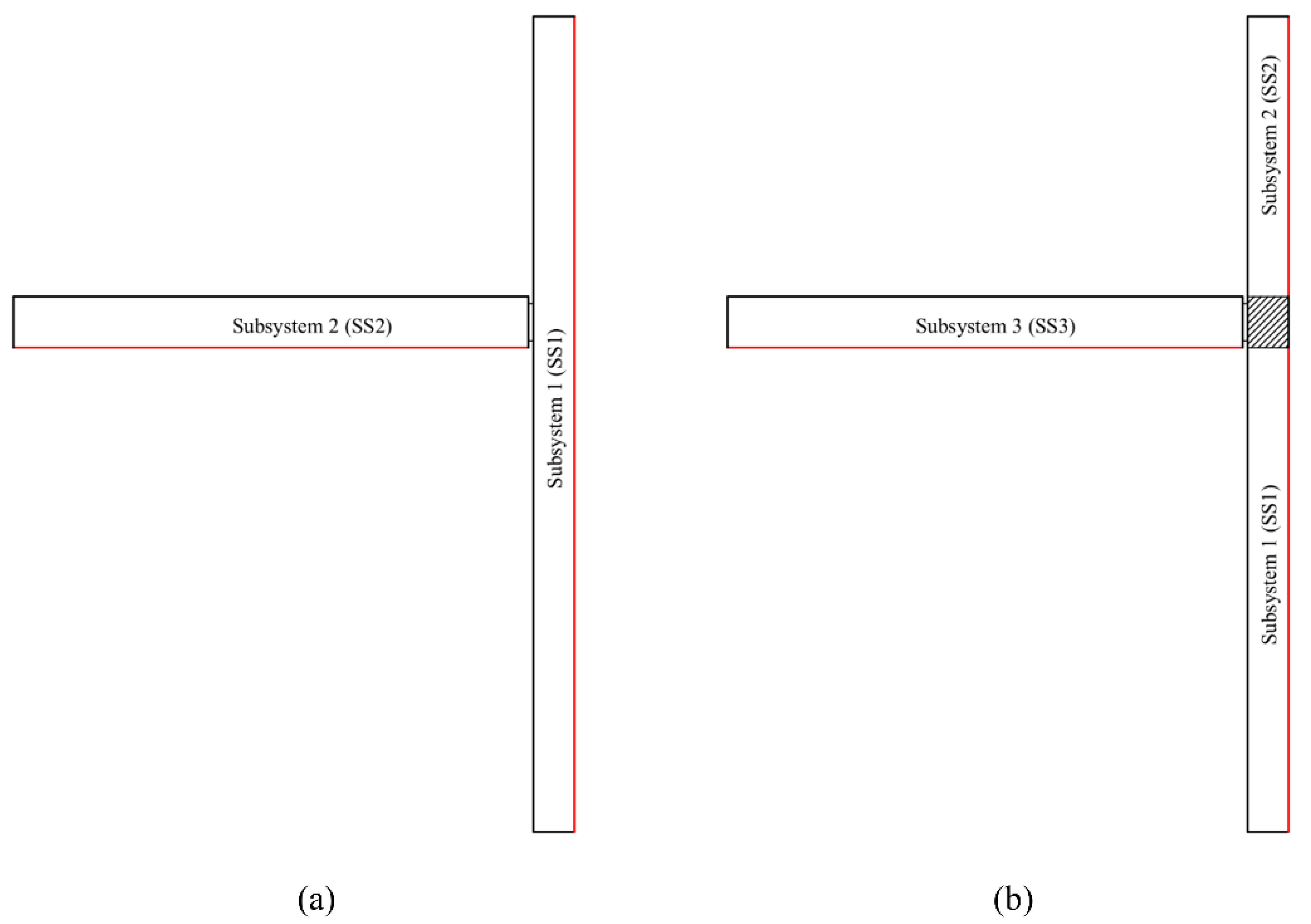
When two subsystems are considered, the beam and the column are each represented by a single subsystem (see Figure 5a). When three subsystems are considered, the beam represents one subsystem and the column is divided into two subsystems at the junction, as indicated in Figure 5b. The output from the FEM models was used to calculate the subsystem energy and power input that would apply to an SEA model for each beam-to-column junction. These FEM data were then used in ESEA to determine coupling loss factors. The beam or column was excited using rain-on-the roof excitation at all of the nodes on the surfaces indicated by red lines in Figure 5.
2.5. T-Junctions—Wave Approach: Bending Waves Only
To validate the FEM models of the beam-to-column junctions, the coupling loss factors resulted from the FEM ESEA of the rigid junction with the inclusion of bending modes only are compared with the CLFs calculated using the wave approach. The coupling loss factor between two beams i and j is
where cg,i is the group velocity for the propagating bending waves on a solid beam i, τij is the transmission coefficient between the beams i and j and Li is the length of beam i.
The transition from thin to thick beam bending theory is expected to occur at ≈400 Hz for the beam and ≈500 Hz for the column. For a Euler–Bernoulli beam (thin beam bending theory), the bending wave group velocity is [26]
where E is the Young’s modulus, I is the moment of inertia, ρ is the density, and A is the cross-sectional area.
For a Timoshenko beam (thick beam bending theory), the bending wave group velocity is [27]
where k1 is the wavenumber, G is the shear modulus, κ is the shear stress distribution parameter which is related to the shape of beam cross-section (κ = 1.2 for rectangular cross section) and ωco is the second spectrum cut-off angular frequency.
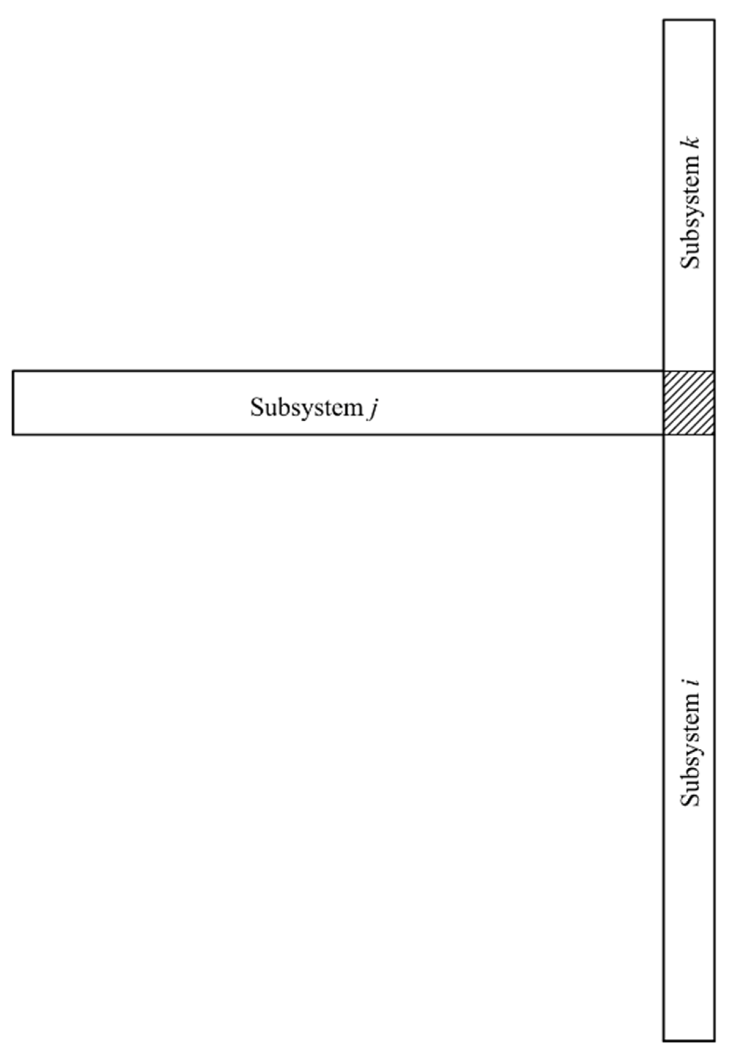
For a beam-to-column T-junction (see Figure 6) the incident bending wave impinges upon the junction at normal incidence, so only the normal incidence transmission coefficient is needed.
Using the subsystem numbering system in Figure 6 with an incident bending wave on subsystem i, the transmission around the corner to subsystem j is given by [28]
where Ji = 2 and Jj = 0.5 when the incident bending wave is on subsystem i and Ji = 2 and Jj = 2 when the incident bending wave is on subsystem j.
The variables χ and ψ are given by [28]
where h is the depth, cL is the quasi-longitudinal phase velocity and ρs is the surface density for subsystems i or j.
3. Results and Discussion
3.1. Mode Count and Modal Overlap
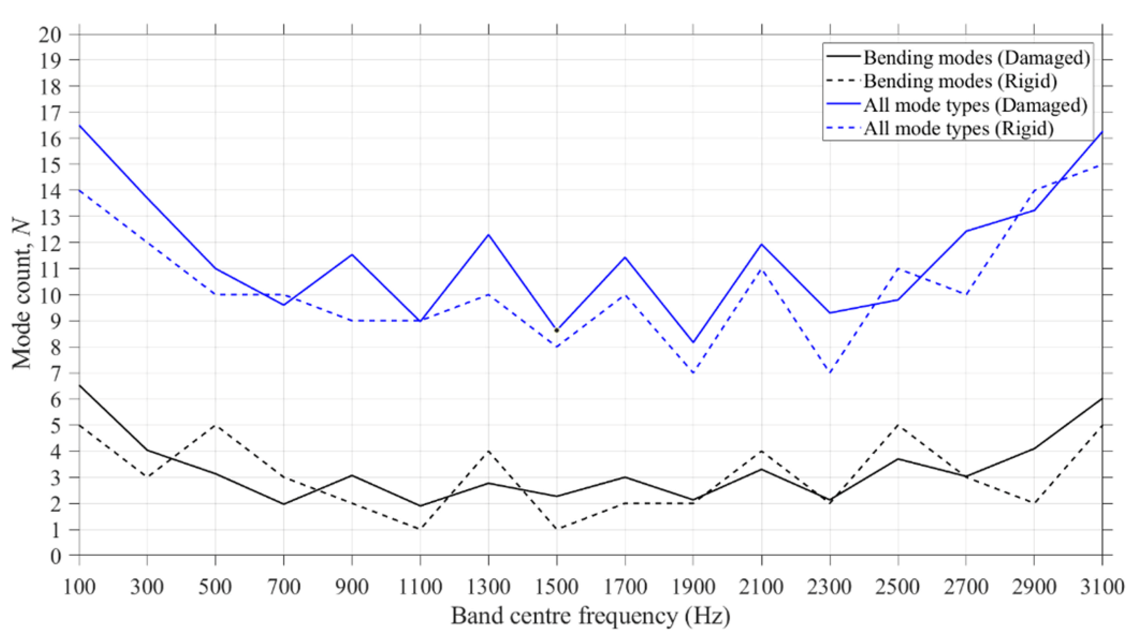
Figure 7 shows the average mode count from FEM in each 200 Hz frequency band for bending modes (out-of-plane) and combinations of all modes for the damaged and rigid beam-to-column junctions. The rigid and damaged T-junctions have similar numbers of bending modes (on average). When all modes are combined, all frequency bands have at least eight and seven modes for the damaged and rigid T-junctions, respectively.
For the rigid junction, Figure 7 indicates that the choice of 200 Hz frequency bandwidths has resulted in all except two frequency bands (1100 Hz and 1500 Hz) having at least two bending modes that determine the response, and therefore the modal overlap factor is estimated to be at least 0.35 in all frequency bands. When SEA is used in a predictive mode with coupling loss factors that are predicted from wave theory, SEA usually relies on modal density estimates that are based on local modes for each subsystem. For coupled plates, Fahy and Mohammad [29] note that a minimum of five modes are needed in a band to give stable estimates of the coupling loss factor. This is because angular average transmission coefficients are used and these are more accurate when there are a sufficient number of modes to cover a wide range of incident angles for the waves that impinge upon a junction. This is not the case for beams where all waves arrive at the junction at a single angle of incidence. Renji [30] emphasised the point that SEA does not ‘require’ a large number of local modes because it is the interaction between the modes of one subsystem in a specified frequency band with those modes in the coupled subsystem; hence, in practice, it is the global modes of the system that determine the response. When SEA is used for coupled beams in a predictive mode with coupling loss factors determined from wave theory, Fahy and Mohammad [29] have shown that wave theory estimates of the coupling loss factor are reasonable when the average modal overlap factor is at least unity. This also ensures low variance in the ensemble. However, Wang and Hopkins [27,31] have subsequently shown that when each beam in a junction or grillage supports at least two local modes for each wave type that occurs in the frequency band of interest and the modal overlap factor is at least 0.1, FEM and measurements tend to have smooth curves such as those predicted with SEA and Advanced SEA (ASEA) using wave theory coupling parameters. Hence the comparison of coupling loss factors from FEM ESEA with the wave approach for the undamaged, rigid T-junction is reasonable.
For the damaged T-junctions, SEA is being used in an experimental mode to determine the coupling loss factors from FEM and as all bands have at least two bending modes and an estimated modal overlap factor ranging from 0.2 to 4.7, it is reasonable to consider the use of SEA.
3.2. Comparison of Coupling Loss Factors from FEM ESEA and Wave Approach for the Undamaged, Rigid T-Junction
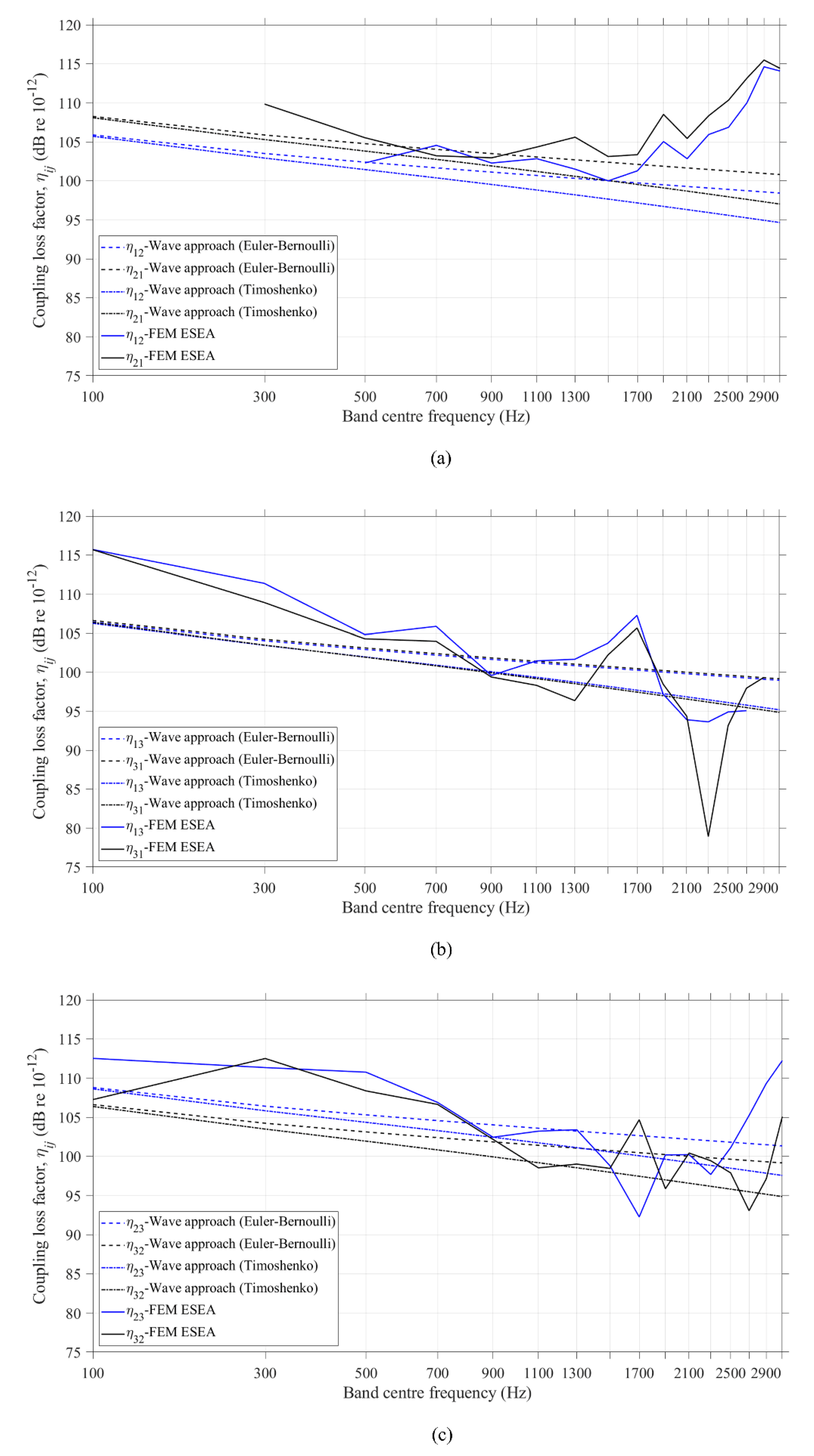
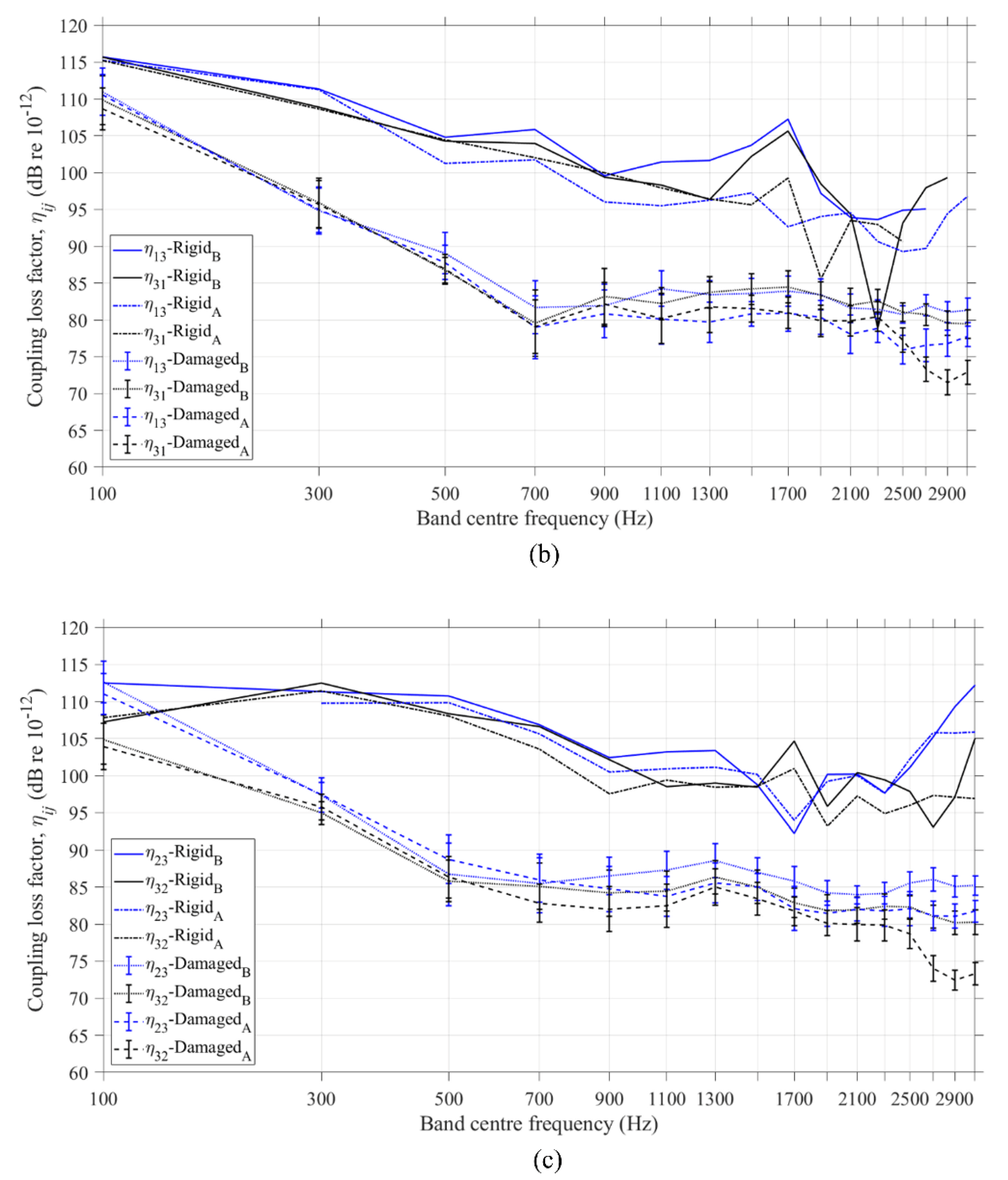
Figure 8a–c compares the coupling loss factors that were determined from FEM ESEA with the wave approach using Euler–Bernoulli and Timoshenko theory (bending waves only) for the undamaged, rigid T-junction. The FEM model has previously been experimentally validated with similar reinforced concrete beams up to 3200 Hz [5,16]; hence, this comparison allows an assessment of the validity of the wave theory as thick beam bending theory (Timoshenko) is expected to be more appropriate above 500 Hz.
Across the straight section of the T-junction (Figure 8a), FEM ESEA resulted in negative CLFs below 500 Hz for η12 and below 300 Hz for η21; hence, these data are not shown on the graph. Note that negative CLFs also occurred in previous work for transmission across the straight section of a T-junction of heavy masonry walls [12]. However, for η12 and η21 between 300 and 1700 Hz, there was reasonable agreement between FEM ESEA and the wave approach using either Euler–Bernoulli theory (differences ≤ 4 dB) or Timoshenko theory (differences within 5 dB). To put this in context, differences of up to 5 dB are common for junctions of heavy masonry walls [18]. Between 2100 and 3200 Hz, the differences increase up to 20 dB.
Around the corner of the T-junction, reasonable agreement (differences within 5 dB) was achieved for η13 and η31 between 500 and 1500 Hz using Euler–Bernoulli theory or Timoshenko theory (see Figure 8b). Around the other corner for η23 and η32 (Figure 8c), nine out of 16 frequency bands between 100 and 3100 Hz achieved reasonable agreement (differences within 5 dB) using the Euler–Bernoulli theory or the Timoshenko theory. As with transmission across the straight section, the differences were also highest at high frequencies for transmission around the corner; these differences were up to 21 dB above 2100 Hz. In addition, the CLFs from FEM ESEA were negative above 2700 and 2900 Hz for η23 and η32, respectively.
In general, the differences can be considered in three ranges. A low-frequency range below 500 Hz with differences up to 10 dB and negative CLFs which might be partly attributed to low modal overlap. The closest agreement occurred in the mid-frequency range (500 to 1500 Hz). In the high-frequency range above 1500 Hz, there were differences larger than 10 dB. As Timoshenko theory should give reasonable estimates at these high frequencies it is likely that the transmission coefficients calculated from Equations (8)–(13) are no longer appropriate at these high frequencies for this thick reinforced concrete junction.
3.3. Coupling Loss Factors from FEM ESEA for Damaged and Rigid T-Junctions
3.3.1. Two Subsystems
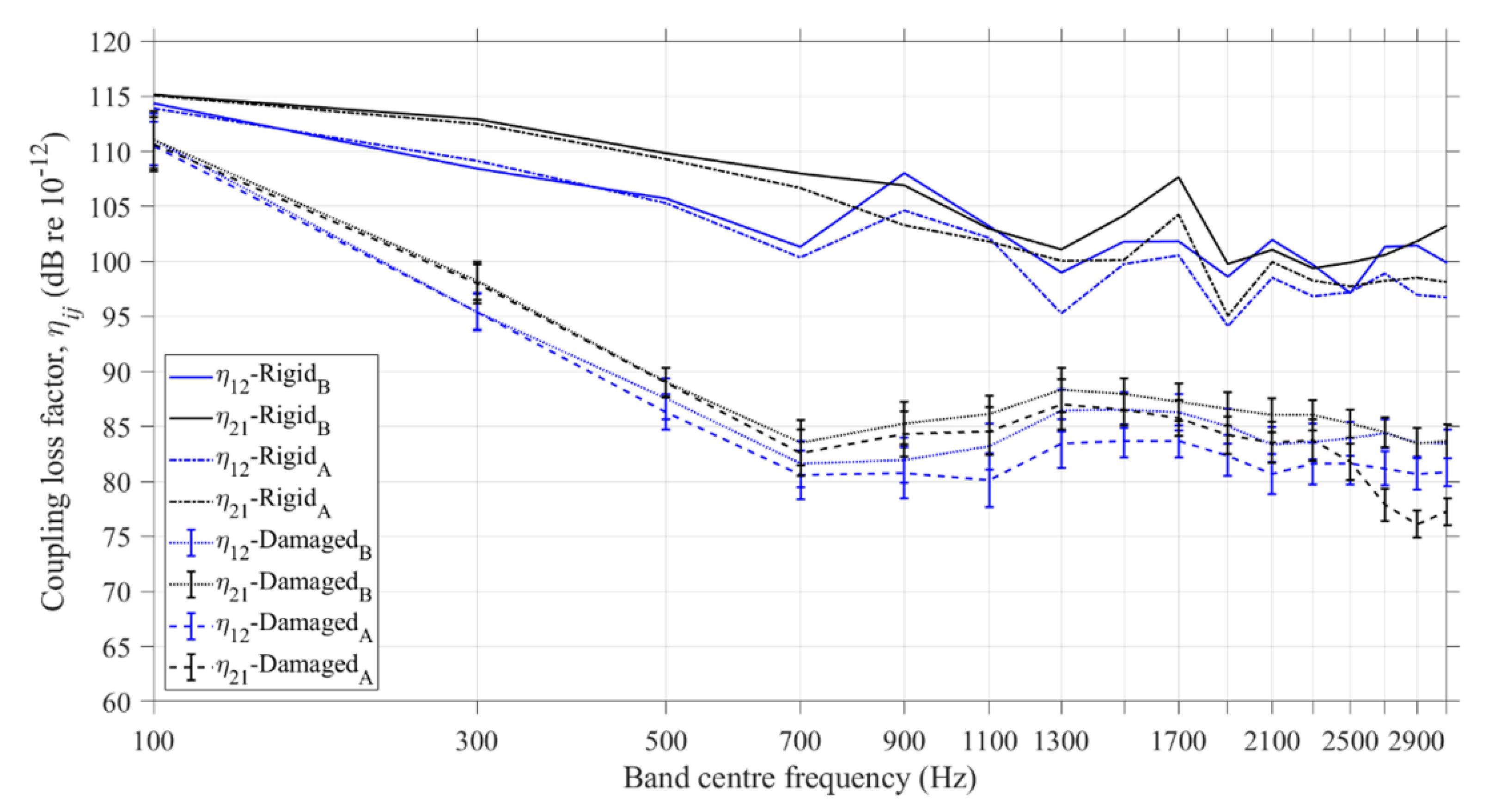
Figure 9 compares the coupling loss factors η12 and η21 from FEM ESEA with two subsystems, considering only bending modes or the combination of all modes in the frequency range from 1 to 3200 Hz. Results are shown for the one undamaged, rigid junction along with the 30 damaged beam-to-column junctions (shown in terms of a mean value with 95% confidence intervals).
Although a rigid junction would rarely be modelled with only two subsystems it is useful to include it here for comparison with the damaged junctions. Differences of up to 5 dB occurred between the CLFs from FEM ESEA with bending modes and the combination of all modes up to 3200 Hz. The higher CLFs with bending modes indicates the importance of these modes for the dynamic response of a beam-to-column junction either if the beam is connected to the column rigidly or only via the steel reinforcement.
For the damaged junctions, the coupling is lower than with the rigid junction, because subsystems 1 and 2 are connected only via the steel reinforcement. For the damaged junctions, the comparison of the CLFs from FEM ESEA with bending modes and the combination of all modes showed close agreement (differences within 5 dB) from 100 to 2500 Hz. Above 2500 Hz, the differences were up to 10 dB. The 95% confidence intervals for the damaged junctions show that the uncertainty is sufficiently low that it should be feasible to estimate the coupling even when the exact angle between the beam and the column is unknown in the damaged junctions of a real collapsed building. For consideration of only bending modes or the combination of all modes, only one junction resulted in negative CLFs in one frequency band of 100 Hz, i.e., 3%.
3.3.2. Three Subsystems
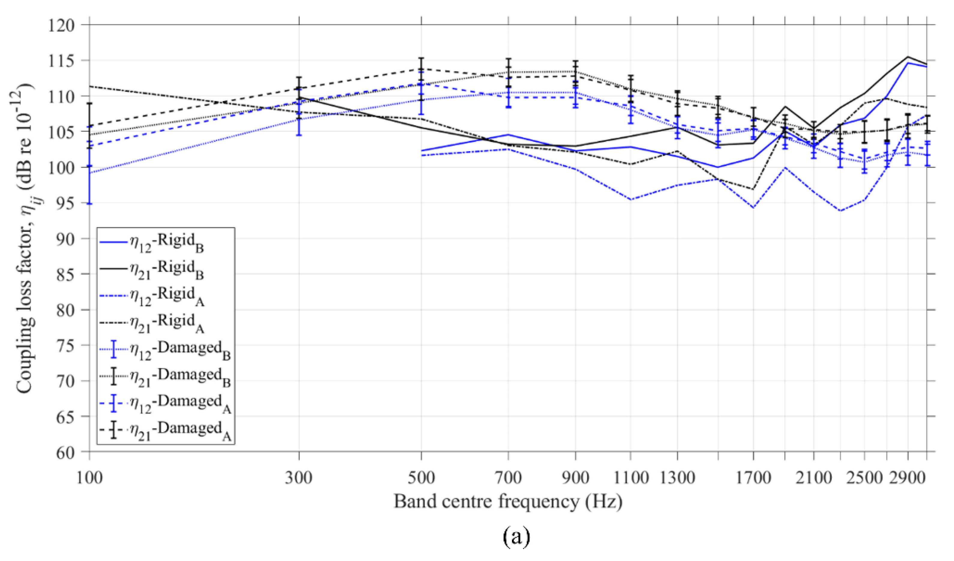
Figure 10a–c allows comparison of the coupling loss factors from FEM ESEA with three subsystems, considering either bending or combination of all modes in the frequency range from 1 to 3200 Hz. Results are shown for the undamaged, rigid junction and damaged junctions. The results for the 30 damaged beam-to-column junctions are shown in terms of a mean value with 95% confidence intervals.
The CLFs η12 and η21 from FEM ESEA with damaged junctions are comparable to the CLFS of the rigid junction (see Figure 10a). This was partially expected since subsystems 1 and 2 are located in the column of the junction where there is no damage. The remaining CLFs (η13, η31, η23, and η32) are smaller in the damaged T-junction than in the rigid one. This is expected because in the damaged junctions, subsystem 3 is connected to subsystems 1 and 2 only via the steel reinforcement and lower coupling is expected (see Figure 10b,c).
For the rigid T-junction, the differences of the CLFs η12, η13 and η31 from FEM ESEA by using bending and combination of all modes were up to 5 dB between 100 and 900 Hz. Above 900 Hz, the differences were between 5 and 10 dB for the vast majority of the frequency bands. For η21, η23 and η32, the differences were typically up to 5 dB over the complete frequency range. FEM ESEA resulted in negative CLFs below 500 Hz and over 2700 Hz, as shown in Figure 10a.
For the damaged junctions, the differences between the CLFs from the FEM ESEA for bending modes only and the combination of all modes were up to 5 dB between 100 and 2500 Hz. Above 2500 Hz, the differences were between 5 and 10 dB. The 95% confidence intervals show that the variation is low; hence, it should be feasible to estimate the coupling even when the exact angle between the beam and the column is unknown in the damaged junctions of a real collapsed building.
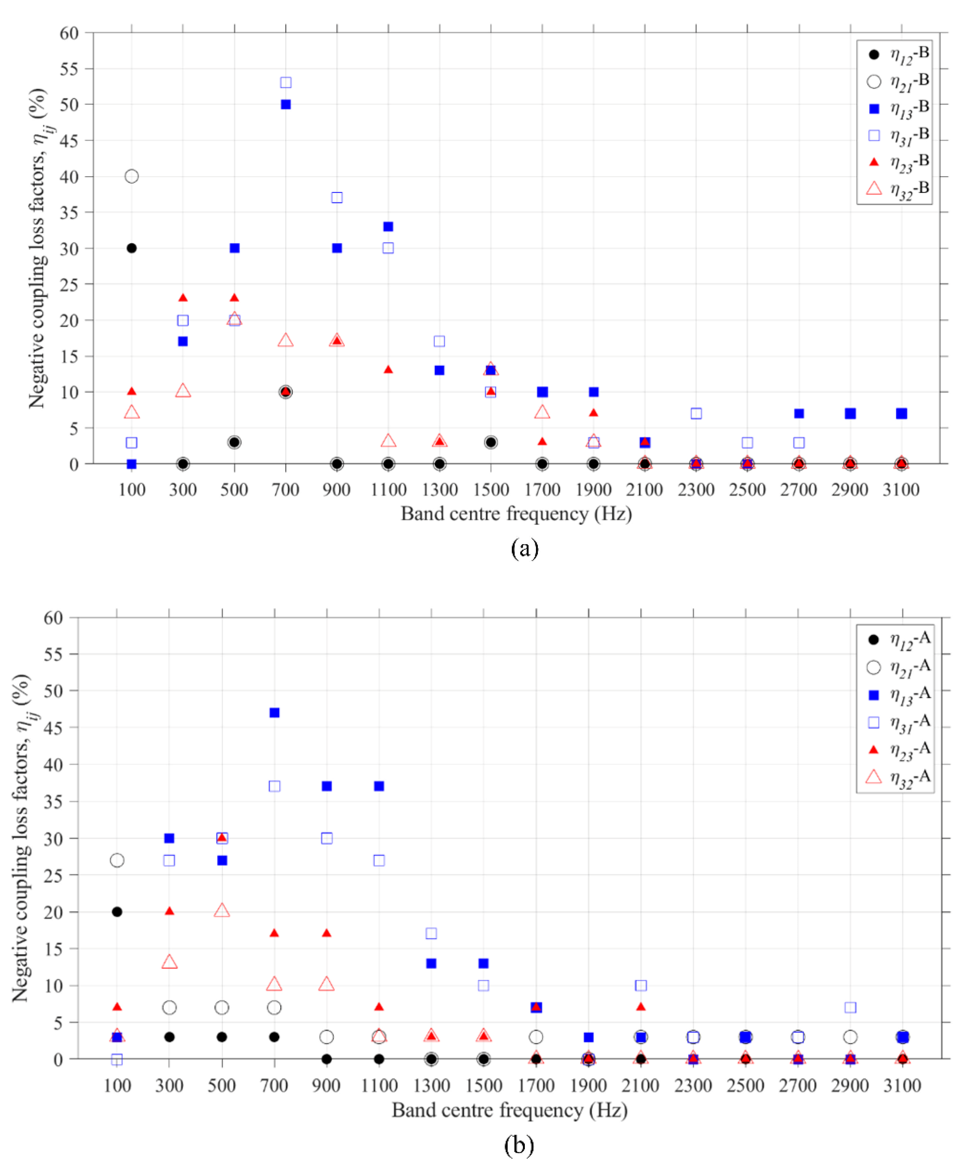
Regardless of the type of modes that are considered (bending modes or the combination of all modes), using three subsystems for the FEM ESEA of the 30 damaged beam-to-column junctions resulted in a significant number of negative coupling loss factors (see Figure 11a,b). Specifically, below 1500 Hz the percentage of the junctions with negative loss factors was between 17 and 54%. These mainly occurred with the CLFs from the column (SS1 and SS2) to the beam (SS3) and vice versa. Above 1500 Hz, the percentage of the junctions with negative loss factors was between 3 and 10%.
For the damaged junctions, the existence of large numbers of negative CLFs below 1500 Hz suggests that the assignment of three subsystems in this frequency range is inappropriate. With a rigid junction there is an impedance change at the junction such that waves are partially reflected but this is not expected in a damaged junction where there is only a connection via the steel reinforcement; hence, a two-subsystem model is more appropriate. Comparing the percentages of negative CLFs from FEM ESEA in Figure 11 with the 3% that occurred with two subsystems, it can be inferred that the use of two subsystems is a more suitable assignment than three subsystems.
4. Conclusions
The output from FEM models of a beam and column junction formed from reinforced concrete have been used with ESEA to assess the potential of creating a SEA model of the junction by calculating CLFs between the beam and column subsystems. To investigate these junctions in a building after earthquake damage, an ensemble of 30 randomly damaged beam-to-column junctions was generated using a Monte Carlo simulation. A rigid T-junction was used as a comparator because the thick reinforced concrete elements were expected to require modelling with Timoshenko theory rather than Euler–Bernoulli theory above 500 Hz. Although the CLFs from FEM ESEA for a rigid T-junction (only bending modes) showed reasonable agreement with wave theory in a mid-frequency range (500 to 1500 Hz), there were differences larger than 10 dB in the high-frequency range above 1500 Hz. FEM models for similar reinforced concrete beams had previously been experimentally validated, hence, it was concluded that the use of Timoshenko theory is not sufficient to model vibration transmission at high frequencies and that the transmission coefficients are no longer appropriate for this thick reinforced concrete junction. This provided additional motivation to use FEM ESEA for damaged junctions because the increased complexity of the fragmented connection at the junction and the existence of more than one wave type which meant that it would be more efficient to use FEM rather than pursue an analytical model based on wave theory for the damaged junction.
Vibration transmission on the damaged junctions only occurs across the yielded steel reinforcement and this does not provide a significant impedance change like the rigid junction. For this reason, ESEA was investigated using either two or three subsystems, i.e., two subsystems where the beam and the column are each represented by a single subsystem or three subsystems where the beam is one subsystem and the column is divided into two subsystems at the junction. Regardless of the number of subsystems and wave types in ESEA, the coupling between the beam and the column was lower in the damaged junction than in the rigid junction. In addition, the use of two instead of three subsystems was shown to be preferable because it significantly decreases the number of negative coupling loss factors from ESEA. This results in a viable SEA model for which the CLFs from FEM ESEA were similar, regardless of whether only bending modes or the combination of all modes were considered in the FEM model (indicating that the bending modes tend to dominate). The ensemble statistics also indicated that that the uncertainty in predicting the CLFs using FEM ESEA is sufficiently low that it should be feasible to estimate the CLF even when the exact angle between the beam and the column is unknown (as would be the case in real buildings after an earthquake).
Author Contributions
Conceptualization, C.H.; methodology, M.F. and C.H.; software, M.F.; formal analysis, M.F. and C.H.; investigation, M.F.; resources, C.H.; writing—original draft preparation, M.F. and C.H.; visualization, M.F.; supervision, C.H.; project administration, C.H.; funding acquisition, C.H. All authors have read and agreed to the published version of the manuscript.
Funding
This research was funded by the EPSRC and ESRC Centre for Doctoral Training in Quantification Management of Risk & Uncertainty in Complex Systems and Environments at the University of Liverpool, grant number 1521238.
Data Availability Statement
The data presented in this study are available on request from the corresponding authors.
Conflicts of Interest
The authors declare no conflict of interest.
References
- Huo, R.; Agapiou, A.; Bocos-Bintintant, V.; Brown, L.J.; Burns, C.; Creaser, C.S.; Devenport, N.A.; Gao-Lau, B.; Guallar-Hoyas, C.; Hildebrand, L.; et al. The trapped human experiment. J. Breath Res. 2011, 5, 046006. [Google Scholar] [CrossRef]
- Macintyre, A.G.; Barbera, J.A.; Smith, E.R. Surviving collapsed structure entrapment after earthquakes: A “Time-to-Rescue” analysis. Prehospital Disaster Med. 2006, 21, 4–19. [Google Scholar] [CrossRef] [PubMed]
- Macintyre, A.G.; Barbera, J.A.; Petinaux, B.P. Survival interval in earthquake entrapments: Research findings reinforced during the 2010 Haiti earthquake Response. Disaster Med. Public Health Prep. 2011, 5, 13–22. [Google Scholar] [CrossRef] [PubMed]
- Bäckström, C.J.; Christofferson, N. Urban Search and Rescue—An Evaluation of Technical Search Equipment and Methods; Lund University: Lund, Sweden, 2006. [Google Scholar]
- Filippoupolitis, M.; Hopkins, C. Experimental validation of finite element models representing stacked concrete beams with unbonded surface contacts. Eng. Struct. 2021, 227, 111421. [Google Scholar] [CrossRef]
- NFPA 1670:2017; Standard on Operations and Training for Technical Search and Rescue Incidents. National Fire Protection Association: Quincy, MA, USA.
- O’Connell, J. Collapse Operations for First Responders, 1st ed.; Penn Well Corporation: Tulsa, OK, USA, 2012. [Google Scholar]
- Schweier, C.; Markus, M. Classification of collapsed buildings for fast damage and loss assessment. Bull. Earthq. Eng. 2006, 4, 177–192. [Google Scholar] [CrossRef]
- Sezen, H.; Whittaker, A.S.; Elwood, K.J.; Mosalam, K.M. Performance of reinforced concrete buildings during the August 17, 1999 Kocaeli, Turkey earthquake, and seismic design and construction practice in Turkey. Eng. Struct. 2003, 25, 103–114. [Google Scholar] [CrossRef]
- Lyon, R.H.; DeJong, R.J. Theory and Application of Statistical Energy Analysis, 2nd ed.; Butterworth-Heinemann: Newton, MA, USA, 1995. [Google Scholar]
- Hopkins, C. Vibration transmission between coupled plates using finite element methods and statistical energy analysis. Part 2: The effect of window apertures in masonry flanking walls. Appl. Acoust. 2003, 64, 975–997. [Google Scholar] [CrossRef]
- Hopkins, C. Statistical energy analysis of coupled plate systems with low modal density and low modal overlap. J. Sound Vib. 2002, 251, 193–214. [Google Scholar] [CrossRef]
- Hopkins, C. Experimental statistical energy analysis of coupled plates with wave conversion at the junction. J. Sound Vib. 2009, 322, 155–166. [Google Scholar] [CrossRef]
- Marshal, J.D.; Lang, A.F.; Baldridge, S.M.; Popp, D.R. Recipe for disaster: Construction methods, materials, and building performance in the January 2010 Haiti earthquake. Earthq. Spectra 2011, 27, 323–343. [Google Scholar] [CrossRef] [Green Version]
- Abaqus 6.14 Documentation and User Manual; Dassault Systèmes Simulia Corporation: Providence, RI, USA, 2014.
- Filippoupolitis, M.; Hopkins, C. Experimental validation of finite element models for reinforced concrete beams with discontinuities that form dowelled-type joints. Vibration 2021, 4, 537–550. [Google Scholar] [CrossRef]
- Atalla, N.; Sgard, F. Finite Element and Boundary Methods on Structural Acoustics and Vibration; CRC Press: Boca Raton, FL, USA; Taylor & Francis Group: Abingdon, UK, 2015. [Google Scholar]
- Hopkins, C. Sound Insulation; Butterworth-Heinemann: Oxford, UK, 2007. [Google Scholar]
- Bies, D.A.; Hamid, S. In situ determination of loss and coupling loss factors by the power injection method. J. Sound Vib. 1980, 70, 187–204. [Google Scholar] [CrossRef]
- Woodhouse, J. An introduction to statistical energy analysis of structural vibration. Appl. Acoust. 1981, 14, 455–469. [Google Scholar] [CrossRef]
- Hodges, C.H.; Nash, P.; Woodhouse, J. Measurement of coupling loss factors by matrix fitting: An investigation of numerical procedures. Appl. Acoust. 1987, 22, 47–69. [Google Scholar] [CrossRef]
- De las Heras, M.F.; Manguán, M.C.; Millán, E.R.; de las Heras, L.F.; Hidalgo, F.S. Determination of SEA loss factors by Monte Carlo Filtering. J. Sound Vib. 2020, 479, 115348. [Google Scholar] [CrossRef]
- Poblet-Puig, J. Estimation of the coupling loss factors of structural junctions with in-plane waves by means of the inverse statistical energy analysis problem. J. Sound Vib. 2021, 493, 115850. [Google Scholar]
- Lalor, N. Practical Considerations for the Measurement of Internal and Coupling Loss Factors on Complex Structures, ISVR Technical Report No. 182. June 1990.
- Jang, H.; Hopkins, C. Prediction of sound transmission in long spaces using ray tracing and experimental Statistical Energy Analysis. Appl. Acoust. 2018, 130, 15–33. [Google Scholar]
- Cremer, L.; Heckl, M.; Ungar, E.E. Structure-Borne Sound; Springer: New York, NY, USA, 1973. [Google Scholar]
- Wang, X.; Hopkins, C. Bending, longitudinal and torsional wave transmission on Euler-Bernoulli and Timoshenko beams with high propagation losses. J. Acoust. Soc. Am. 2016, 140, 2312–2332. [Google Scholar] [PubMed]
- Craik, R.J.M. Sound Transmission Through Buildings: Using Statistical Energy Analysis; Gower Publishing Limited: Hampshire, UK, 1996. [Google Scholar]
- Fahy, F.J.; Mohammed, A.D. A study of uncertainty in applications of SEA to coupled beam and plate systems. Part 1: Computational experiments. J. Sound Vib. 1992, 158, 45–67. [Google Scholar] [CrossRef]
- Renji, K. On the number of modes required for statistical energy analysis-based calculations. J. Sound Vib. 2004, 269, 1128–1132. [Google Scholar] [CrossRef]
- Wang, X.; Hopkins, C. Experimental and numerical validation of Advanced Statistical Energy Analysis to incorporate tunneling mechanisms for vibration transmission across a grillage of beams. Acta Acust. 2022, 6, 51. [Google Scholar] [CrossRef]
Figure 2.
Geometry and reinforcement details of: (a) an undamaged and (b) a damaged beam-to-column junction (units: millimetres).
Figure 2.
Geometry and reinforcement details of: (a) an undamaged and (b) a damaged beam-to-column junction (units: millimetres).

Figure 3.
Cross-sections of the reinforced concrete members: (a) beam and (b) column (units: millimetres).
Figure 3.
Cross-sections of the reinforced concrete members: (a) beam and (b) column (units: millimetres).

Figure 4.
(a) FEM model of a rigid beam-to-column T-junction and (b) FEM model of a damaged beam-to-column T-junction. The orange symbols indicate the positions of the simple supports.
Figure 4.
(a) FEM model of a rigid beam-to-column T-junction and (b) FEM model of a damaged beam-to-column T-junction. The orange symbols indicate the positions of the simple supports.

Figure 5.
Subsystem allocation for the beam-to-column junctions: (a) two subsystems and (b) three subsystems. The red lines indicate the surfaces where the rain-on-the-roof excitation is applied and the response is measured.
Figure 5.
Subsystem allocation for the beam-to-column junctions: (a) two subsystems and (b) three subsystems. The red lines indicate the surfaces where the rain-on-the-roof excitation is applied and the response is measured.

Figure 6.
Subsystem numbering for the beam-to-column T-junction for the application of the wave approach.
Figure 6.
Subsystem numbering for the beam-to-column T-junction for the application of the wave approach.

Figure 7.
Comparison of the average mode count of the 30 damaged junctions with the mode count of the T-junction for out-of-plane bending modes and combination of all mode types.
Figure 7.
Comparison of the average mode count of the 30 damaged junctions with the mode count of the T-junction for out-of-plane bending modes and combination of all mode types.

Figure 8.
Comparison of FEM and the analytical (wave approach) coupling loss factors for the undamaged, rigid T-junction: (a) η12 and η21, (b) η13 and η31 and (c) η23 and η32.
Figure 8.
Comparison of FEM and the analytical (wave approach) coupling loss factors for the undamaged, rigid T-junction: (a) η12 and η21, (b) η13 and η31 and (c) η23 and η32.

Figure 9.
Coupling loss factors η12 and η21 resulting from FEM ESEA using two subsystems with bending modes only (B) and the combination of all modes (A). Error bars denote the 95% confidence intervals.
Figure 9.
Coupling loss factors η12 and η21 resulting from FEM ESEA using two subsystems with bending modes only (B) and the combination of all modes (A). Error bars denote the 95% confidence intervals.

Figure 10.
Coupling loss factors resulting from FEM ESEA with three subsystems for bending modes only (B) and the combination of all modes (A): (a) η12 and η21, (b) η13 and η31 and (c) η23 and η32. The error bars denote the 95% confidence intervals.
Figure 10.
Coupling loss factors resulting from FEM ESEA with three subsystems for bending modes only (B) and the combination of all modes (A): (a) η12 and η21, (b) η13 and η31 and (c) η23 and η32. The error bars denote the 95% confidence intervals.


Figure 11.
Damaged junctions—Percentage of negative CLFs resulting from FEM ESEA with: (a) three subsystems for bending modes only (B) and (b) three subsystems for the combination of all modes (A).
Figure 11.
Damaged junctions—Percentage of negative CLFs resulting from FEM ESEA with: (a) three subsystems for bending modes only (B) and (b) three subsystems for the combination of all modes (A).


Table 1.
Material properties.
| Material | Density, ρ [kg/m3] | Young’s Modulus, E [N/m2] | Poisson’s Ratio, ν [–] |
|---|---|---|---|
| Concrete | 2287 | 34.7 × 10⁹ | 0.2 |
| Steel | 7800 | 200 × 109 | 0.3 |
Disclaimer/Publisher’s Note: The statements, opinions and data contained in all publications are solely those of the individual author(s) and contributor(s) and not of MDPI and/or the editor(s). MDPI and/or the editor(s) disclaim responsibility for any injury to people or property resulting from any ideas, methods, instructions or products referred to in the content. |
© 2023 by the authors. Licensee MDPI, Basel, Switzerland. This article is an open access article distributed under the terms and conditions of the Creative Commons Attribution (CC BY) license (https://creativecommons.org/licenses/by/4.0/).
Share and Cite
MDPI and ACS Style
Filippoupolitis, M.; Hopkins, C. Vibration Transmission across Seismically Damaged Beam-to-Column Junctions of Reinforced Concrete Using Statistical Energy Analysis. Vibration 2023, 6, 149-164. https://doi.org/10.3390/vibration6010011
AMA Style
Filippoupolitis M, Hopkins C. Vibration Transmission across Seismically Damaged Beam-to-Column Junctions of Reinforced Concrete Using Statistical Energy Analysis. Vibration. 2023; 6(1):149-164. https://doi.org/10.3390/vibration6010011
Chicago/Turabian StyleFilippoupolitis, Marios, and Carl Hopkins. 2023. "Vibration Transmission across Seismically Damaged Beam-to-Column Junctions of Reinforced Concrete Using Statistical Energy Analysis" Vibration 6, no. 1: 149-164. https://doi.org/10.3390/vibration6010011