1. Introduction
Moving load problems have attracted the scientific community for many years since the first railway lines were built. Numerical models of railway tracks are essential tools for studying their dynamic behavior with implications for the safety and comfort of railway transport. The importance of these models has increased in recent decades due to the intensified attention that must be paid to the environment and its protection, as well as due to the increase in the speed of rail vehicles, the weight of the load, and the capacity of the network.
Despite the widespread use of detailed finite element models, reduced models are still important for their ease of application, results interpretation, and low computational cost. In this contribution, the classification of reduced models according to [
1] will be used, namely, one-, two- and three-layer models will be analyzed. It is of note that the one-layer model is in fact a beam supported by the Winkler-Pasternak foundation.
Advances in symbolic software have renewed interest in semianalytical solutions, thus, this paper aims to highlight the importance and power of analytical and semianalytical methods and results. This is because there are several advantages associated with these methods, some of which are listed below:
They can provide better insight into physical phenomena because the origin of each part of the final result is traceable.
They provide fast calculation, especially when the solution is presented by closed-form formulas.
They provide highly accurate results at once, as no additional numerical convergence tests are needed.
The obtained results are easy to analyze, because due to necessary simplifications, they are limited to an essential part.
Only the part of the model that is needed can be evaluated, and such restrictions can be made in space and/or time, because there is no need to track the full-time history.
The formulations used are suitable for dimensionless parameters, allowing one to visualize in one graph all possible results for all possible combinations of data.
Dimensionless parameters have predictable and numerically stable values.
Closed-form results allow direct parametric or sensitivity analyses.
Of course, there are also several disadvantages related mainly to the structure and analysis to which these methods can be applied.
Moving load problems are fundamental problems in structural dynamics. However, it is crucial to distinguish whether inertial effects are considered in the moving object or not. This imposes differences in the solution methods and in undesirable phenomena that can occur. Therefore, it is necessary to use moving forces more correctly and distinguish these cases from moving masses or oscillators. Assuming a linear longitudinally homogeneous infinite structure, the basic differences are as follows: (i) When moving forces are considered, the steady-state regime is easily reached; therefore, solution methods may neglect transient vibration and the initial instant is not very important. Additionally, superposition is possible, so the problem can be solved for one moving force, and then the results superimposed to obtain the response for a set of forces. (ii) When moving masses or oscillators are considered, the transient vibrations cannot be omitted because then the instability problems would remain completely hidden. Thus, the initial instant is vital and deflection shapes must be tracked from the very beginning. Superposition of results is not possible if the moving objects are not completely apart. For proximate objects, the dynamic interaction is of utmost importance, as it can significantly influence instability conditions.
Published works on instability problems are generally devoted to infinite structures. In [
2,
3], the conditions for instability are determined by the D-decomposition method, but the full forms of beam deflection are not given. The mass is assumed to be in permanent contact with the beam. A nonlinear contact spring is introduced in [
4,
5]. The shapes of the deflections are determined numerically, and the instability is again analyzed by the D-decomposition method.
A pioneering solution about a sequence of masses traversing a finite beam was presented in [
6,
7]. In [
8], the problem was solved by the double Fourier transform, hiding this way the possibility of instability. Solution with the help of Green’s function and the D-decomposition method is presented in [
9] with the aim to determine the instability conditions of a sequence of moving oscillators on an infinite beam. The D-decomposition method is also used in recent work [
10]. While in [
9] a contact spring was used, in [
10] it was again assumed that the moving mass is in permanent contact with the beam. Nevertheless, none of these works is concerned with the damping influence on the dynamic interaction, which requires further consideration from an analytical point of view. It is important to derive conditions under which results can be superposed and identify cases where the dynamic interaction induces instability at a lower velocity than the lowest critical velocity of the moving force, [
11,
12].
Several recent works about constant force moving on an infinite structure are exploiting semianalytical methods. Fully analytical expressions are derived in [
13,
14]. The aim of these two works is very similar; there are only some differences in the characterization of the Winkler-Pasternak foundation and the critical damping. Both papers are also focused on critical velocity.
The wavelet transform is implemented in [
15] to analyze the problem of moving forces on a double-beam model. The Adomian decomposition is implemented to deal with the nonlinearity of the viscoelastic layer connecting the two beams. The model is further modified to the two-layer model in [
16] and extended to include nonlinearity in the foundation [
17,
18]. In all these works, the steady-state regime is derived directly. A comparison with experimental measurements is conducted in [
16,
17,
18].
The three-layer model and its applicability to represent full finite element models is dealt with in [
19] and the question of the critical velocity of the moving force is briefly discussed.
Several works deal with finite beams on Winkler or Winkler–Pasternak foundation with external linear viscous damping. The moving oscillator is studied in [
20], and the internal hinge and variable velocity are analyzed in [
21] by an improved perturbation technique applied to governing stochastic equations. The modified finite element method is introduced in [
22] on functionally graded simply supported Timoshenko beam on Winkler–Pasternak foundation subjected to a moving mass crossing the beam by variable velocity. A very long finite three-layer model is considered in [
23]. The modal expansion method is applied to a reduced model to increase the computational efficiency. A control volume is introduced to reduce the computational domain and the structure is traversed by a multi-body model of the vehicle.
Fewer works are published on infinite beams. Pioneering work on the mass moving on an infinite Winkler beam is given in [
24]. The problem is solved by integral transforms, with numerically performed the inverse one. In [
25], integral transforms lead directly to the steady-state regime, removing the inertial effect in the moving object and hiding the possibility of instability. An inhomogeneous Winkler foundation with smooth variation is introduced in [
26,
27]. The structure is crossed by a moving force in [
26] and by a moving oscillator in [
27]. In [
28], a comparison of possible methods for solving similar problems is presented. A novel model for the dynamic interaction of the beam with its foundation is introduced in [
29]. Governing equations are derived from the extended Hamilton principle. A nonlinear elastic constitutive relationship connects the Winkler and Pasternak moduli which are further obtained as a part of the solution. It is shown that these moduli are not constant but time-dependent because they are influenced by the beam–foundation interaction. In addition, the dynamically activated mass of the foundation is also obtained as a part of the solution.
The approach to detect instability used in this paper is
conceptually different from previous works by other researchers, and therefore several new terms need to be introduced. One of the fundamental ones is the so-called
mass-induced frequency (MIF), which is defined as a complex root of a complex characteristic equation. It must be distinguished from natural frequency because it depends on the mass that is moving and its velocity.
Frequency lines is also a new term used for sets of MIFs for a given case as a function of velocity. While the D-decomposition method identifies the number of roots leading to instability, in the semianalytical approach presented here, the roots are actually determined, they are MIFs with negative imaginary parts, and the instability intervals are delimited by the so-called
instability lines. MIFs can further be used to characterize the vibration shapes of the entire beam during the transient regime and in unstable cases can help evaluate the severity of the instability, which is important for mitigation measures. MIF was first introduced in [
30] and the necessity of branch cuts and the definition of
discontinuity lines were introduced in [
31].
Other new terms are related to the critical velocity of the moving force, the so-called
pseudo-critical velocity (PCV) was first introduced in [
32] and further analyzed in [
33]. A new term introduced for the first time in this paper is the
false critical velocity (FCV), the existence of which will be explained in the context of finite beams based on the analyses presented in [
34]. In addition to this new concept, the contribution of this manuscript is the analysis of the three-layer model focusing on the critical velocity of the moving force and instability of the moving mass. While the techniques are based on the same steps as for the simpler models, the application is new. Owing to more complicated behavior, additional new terms are introduced, namely the
false onset of instability (FOI) and
false end of instability (FEI).
The paper is organized as follows: in
Section 2, the layered models of the railway track are defined together with the necessary descriptions and simplifying assumptions.
Section 3 presents the governing equations for general loads.
Section 4 is devoted to the critical velocity of the moving force, while
Section 5 deals with the instability of moving inertial objects. The main conclusions of the study are presented in
Section 6.
2. Layered Models of Ballasted Railway Tracks
This contribution deals with reduced models of railway tracks, which can be classified as one-, two- and three-layer models according to [
1]. All of them are still widely used due to their computational efficiency and a reasonable approximation of reality, which is confirmed especially with the three-layer model. These models are depicted in
Figure 1.
The following description applies: All models in
Figure 1 are considered infinite and have a guiding structure in form of a beam standing for the rail and modeled according to the Euler-Bernoulli theory, and therefore characterized by the bending stiffness (
) and the mass per unit length (
). The possibility of applying an axial force (
) assumed positive when inducing compression is also included. All models have a foundation layer characterized by its vertical stiffness (
) and viscous damping (
), but the physical interpretation is different because these values must represent all layers below the last modeled one. The two-layer model additionally includes rail pads, described by their vertical stiffness (
) and viscous damping (
); and sleepers included as point masses (
). The three-layer model additionally contains the ballast layer, characterized by its vertical stiffness (
), viscous damping (
) and mass (
), which is dynamically activated. All models have a certain shear stiffness. In the one-layer model, this is modeled by a shear layer characterized by the Pasternak modulus (
). Therefore, this model is actually the classical Winkler-Pasternak beam. It is useful to recall that the shear layer can be equivalently modeled by rotational springs. In the two-layer model, there is no physical place to allocate a shear component. It cannot be added to the foundation as in the one-layer model, because the rotational degree of freedom is not transmitted. Therefore, it is added in the form of vertical springs acting as a shear component between sleepers, (
). This does not mean that there is a shear interaction between sleepers, this is just for modeling purposes as the model has to have some shear stiffness or it would be detached from reality. In the three-layer model, the shear component is added to ballast and has full physical meaning, (
)
For the effective application of the proposed method, one of the main assumptions states that all supports are continuous. Therefore, all the above values stand for distributed values. Thus, for example, if one has data for rail pads and knows the distance between sleepers (), these values are divided by . The same applies to sleepers’ mass. Since only one rail is modeled, the mass of half the sleeper is divided by to be uniformly distributed. As for the ballast, the corresponding values are usually determined by the stress cone theory and then divided by . and viscous damping are usually specified as distributed. The shear component must be treated differently, as it is basically connected in series and not in parallel similar to the other components, and therefore needs to be multiplied by , except for the Pasternak modulus, which is usually introduced as distributed. All models are thus longitudinally homogeneous. This does not represent a significant limitation since discrete supports can be equivalently modeled by the harmonic component of the moving force. Anyway, significant differences in behavior are only apparent at high frequencies, around the pinned-pinned frequency.
In addition to the axial force, two masses, on which constant forces act, are moving on the beam at constant velocity . The distance between them is denoted as . The number of unknown deflections corresponds to the number of layers, but attention will be paid mainly to the beam deflection, . Another simplifying assumption is that the masses are always in contact with the beam.
Analyses will focus on:
determination of the critical velocities of the moving force;
determination of the onset of instability of the moving mass;
the relationship between the two previous findings;
change in instability due to dynamic interaction of proximate moving masses.
4. Critical Velocity of a Moving Force
The critical velocity (CV) of a moving force is a resonance-type phenomenon. It is defined as follows: Assume a constant moving force traversing a guiding structure (usually in the form of a beam) at a constant velocity. The guiding structure is placed on a supporting medium, homogeneous in its longitudinal direction. The analysis of this scenario should be conducted in the purely undamped case. Then, if the force is moving at the CV, there is no steady-state solution. The transient solution increases indefinitely as time increases and never stabilizes. In other words, the beam deflection increases gradually to infinity, similar to the amplitude of a harmonic oscillator under a harmonic force whose excitation frequency is equal to the natural frequency of the oscillator, which justifies the use of “resonance” in this context. The term resonance is also used e.g. in [
14]. However, the solution exists for infinitely lower velocity as well as infinitely closest, but higher one. Depending on the model, there may be more CVs. CV also indicates the separation between different deformation shapes of the beam. Up to the lowest CV, the shape of the beam deflection is perfectly symmetrical with the maximum value at the position of the moving force, the so-called the
active point (AP). There is a noticeable difference between the maximum and minimum deflections along the whole beam. For velocities higher than the lowest CV, there is a sudden jump to zero deflection at the AP and an infinite wave is formed ahead and behind the AP. This also means that the maximum and minimum deflections along the whole beam are the same. Some researchers do not consider this shape to be a valid solution because it violates the boundary conditions at both plus and minus infinity, [
14], but it can be considered a valid solution for the limiting case for infinitesimally small damping.
For this analysis, the initial instant is not really important, and it is possible to reduce the solution method to lead directly to the steady-state solution, since during the transient part of these vibrations, the steady-state shape is smoothly reached without any danger of further side effects.
The moving force problem has another advantage: with linear properties, superposition of results is possible, so that one moving force can be solved and then the solution can be easily extended for a set of moving forces.
CVs are analytically determined as the velocities at which a real double pole exists in Fourier space. Therefore, the solution method follows these steps. First, switching to moving coordinates is performed with
. Considering that the goal is to obtain a steady-state solution, the time-dependent terms can be neglected. Then it follows for the three models.
The next step consists of introduction of dimensionless parameters. The beam with bending stiffness
, distributed mass
and foundation stiffness
is selected as the reference Winkler beam. Then:
where
identifies the critical velocity of the moving force traversing such a reference beam and
designates the velocity ratio. Furthermore, dimensionless spatial coordinate and time are defined as:
The deflection fields are presented as the ratio of the maximum static deflection exerted by force
on the reference beam, therefore:
Further, mass and stiffness ratios are:
damping ratios read as:
and axial and shear force ratios are:
Finally, the moving mass and force ratios are:
Defining the moving force ratio is certainly abundant, but mathematically more correct and suitable for further generalizations. The dimensionless forms of Equations (4)–(6) are given below
The Fourier transform can then be applied
leading to
where
This allows oneto analytically calculate the Fourier image of the displacement fields. The inverse Fourier transform can also be performed analytically, and the steady-state shape can be calculated semianalytically by contour integration. But now the aim is to determine the CVs. To this end, all damping ratios are zero, so all imaginary terms are eliminated. The existence of the real double pole can be written as a system of two equations. This system can be simplified and analytically solved for the one-layer model and, in the absence of the shear component and axial force, for the remaining two models as well. If an analytical solution is not possible, predefined functions in Maple can be used to solve for the roots. The steps to follow are described below.
For the one-layer model (taking into account that
, and substituting
The second equation can be multiplied by
and subtracted from the first one. Knowing that
must be real, then
. Substituting into the second equation, the well-known formula is obtained [
14,
35,
36].
For the two-layer model, the determinant of Equation (19) must be considered, and the same steps can be performed. The determinant can be written as a cubic polynomial for
and the second equation as a quadratic polynomial for
In order to express directly
, the second equation, multiplied by
, should be subtracted from the first one multiplied by 2. Then
For
Equation (31) simplifies to
and by substituting it back into the second equation of the system (30), one can obtain a cubic equation for
, which the discriminant is
There are three simple real roots when the discriminant is positive, which can be substituted back into Equation (32). Then it is also necessary to check that all these roots are positive and lead to a positive number when substituted back into Equation (32). Then, there are at most three
-values of resonance which are defined by analytical formulas. More details are in [
12].
In the general case, i.e., when and/or , the second equation of system (30) leads to a sixth-order polynomial for , which is not written here due to its length, nevertheless, at most three solutions lead to valid and , more precisely, either one or three.
For the three-layer model, the equations to be solved can be established in the same way, but now, polynomials are of a higher degree, and it is not possible to do a simple analysis of the nature of the roots. There can be one, three, or five valid and -values.
Now the question is what happens when the number of values is not complete, and it is also necessary to check that all values leading to resonance have the expected properties of the CV. The first question can be answered by parametric analysis. Such tests reveal that when the number of expected values is not complete, there are some peak deflections at the AP, but these values are not analytically infinite. Such
-values will be called pseudo-critical velocities (PCVs) [
32,
33]. The second question can be answered by analysis of finite beams. To do this, it is first necessary to determine the undamped natural frequencies of the equivalent finite models. For finite models, moving coordinates are not convenient. The free vibrations are thus described by
Admitting harmonic vibrations
,
and
, where
and the mode shapes in the form of
,
and
(no ambiguity is possible, therefore same designations can be used), one obtains
Thus, after removing damping the only change with respect to
is the switch of
to
. Additionally, for instance, for a simply supported beam
, but for our purpose it is more convenient to continue with
. The natural frequencies are solved from the nullity of the respective determinants. That is, for the one-layer model
The resonance condition is defined by the equality of the excitation frequency with the natural frequency
And thus, the CV should correspond to
at a local minimum. Knowing that
must be real and positive
Moreover, the second derivative is positive at the stationary point, confirming that lies at the global minimum in this case. It is necessary to highlight that , otherwise, instability of the beam may occur, thus the solution given by Equation (42) is always valid.
Similar steps can be performed for the two-layer model. Now quadratic equation for
is obtained.
where
And thus
Then the resonance condition must be written for these two frequencies. Each frequency leads to several stationary points. They can be substituted back to obtain
-values at resonance. However, when analyzing them numerically, at most three of them give valid values, more precisely one or three. Sorting them can verify that the first and third values identify the local minima, while the middle value identifies the local maximum. Furthermore, the analysis of the deflection shapes confirms that the middle value does not verify the expected characteristics of the CV for the closest
-values infinitely higher, such as a sudden jump to zero deflection at the AP, as well as the same global maxima and minima over the whole beam. Such values are called the false critical velocities (FCVs). But they still mark resonance, thus there is no solution for such
, because the deflection tends to infinity, like in other cases. More details on the connection between the critical velocity of finite and infinite models can be found in [
34].
For the three-layer model, the determinant of Equation (39) leads to a cubic equation for
where
therefore Equation (46) can also be solved analytically and there will be three simple real solutions if the discriminant is positive. The analytical solution is not written here due to its length.
By introducing the resonance condition, it can be confirmed that each frequency leads to several stationary positions, but at most five in total correspond to valid and . More specifically, there are only one, three, or five valid values. As before, when ordered, odd values identify CVs and even FCVs. In the example section, it will be shown that there are no FCVs between PCVs and CVs, they only appear between two CVs.
5. Moving Inertial Objects
5.1. Solution of the Problem
When a moving object has inertia, the solution method needs to be adapted. Whether for a moving mass or a moving one- or two-mass oscillator or a more complex model, the initial instant is important and cannot be omitted. Omitting it would remove all inertial effects from the moving object and yield a steady-state solution, as for a moving force. This would hide the possibility of instability, and if instability did occur, a steady solution would not be achieved and thus the whole solution would be wrong. To capture the initial time instant, firstly, after switching to moving coordinates, the time-dependent terms cannot be omitted. Then the Laplace transform must be applied first
The Laplace counterpart of
is
, where
is frequency, but
is used in Equation (48) to preserve the correct formalism. The Fourier transform is then applied. Under homogeneous initial conditions, there will be the following differences with respect to the previous analysis: on the left-hand side everything looks formally the same, only functions
now also depend on
and each occurrence of
changes to
.
On the right-hand side, one obtains for one moving mass
which means that the Laplace image of the beam displacement at the AP,
, must be solved and removed. First, the governing equations must be solved for
where
is the determinant of the whole system and
is the subdeterminant obtained by cutting the first row and the first column. For the one-layer model, there is no such subdeterminant, so unity is used instead.
Now, one can perform the inverse Fourier transform to retrieve the Laplace image
By introduction of
it follows that
and after substitution back
Equation (61) holds for all three models. It is just seen that the difference between models is based on the -function, which is proportional to the equivalent flexibility of these models. coordinate is only needed for full deflection shapes, the main analyses that follow require only values of for a given and its variation along the -complex plane.
In conclusion, an analytical expression for the Laplace image of the beam displacement is given by Equation (61). To perform the inverse transform, the definition
is used, where
is a small number. Likewise, as in the previous works, it was found to be more convenient to switch the real and imaginary axes, so the final beam deflection shape can be calculated numerically as
and in this case
must be chosen so that all the discontinuities and poles of the function to be integrated must be located above the line
in the
-complex plane, which is easily accomplished, as will be seen in other sections. First, all discontinuities are located in the real part of the
-complex plane and the poles can be calculated in a fairly simple way, especially those with a negative imaginary part. Then
must be higher than the absolute value of the lowest negative imaginary part of the
-poles.
5.2. Discontinuity Lines
The discontinuity lines indicate the places in the complex -plane where the -function exhibits a discontinuity. This is important for the next sections and can be conducted by the analysis of . For a given , is a fourth-, sixth- or eighth-order polynomial in , if related to a one-, two- or three-layer model, respectively. Discontinuities in the -function occur whenever the nature of the -roots changes. Any such change must go through a situation where there is a real -root, which causes a jump, especially in the imaginary part of the -function.
To find
for which there is a real
-root, for a given
, and other model characteristics, one can assume that
and that
can be written as
where
is the unknown real root, which can be positive or negative. By introducing
into
, one obtains an expression independent of
. For
a similar situation occurs. By comparing the real and imaginary parts of these two equations, it can be observed that the real parts are equal, and the imaginary parts are opposite. Since these equations must be equal to zero, it is possible to impose nullity separately on their real and imaginary parts and deal with
only, for instance. Then, for a chosen value of
,
and
can be solved as real roots of two equations with real coefficients, which is generally an easy task. After that
and
can be substituted back indicating the
where the discontinuity that was searched for occurs. The advantage, besides the ease of implementation, is that
and
can be solved only once (for each
) and then
can be determined for each
simply using Equation (64).
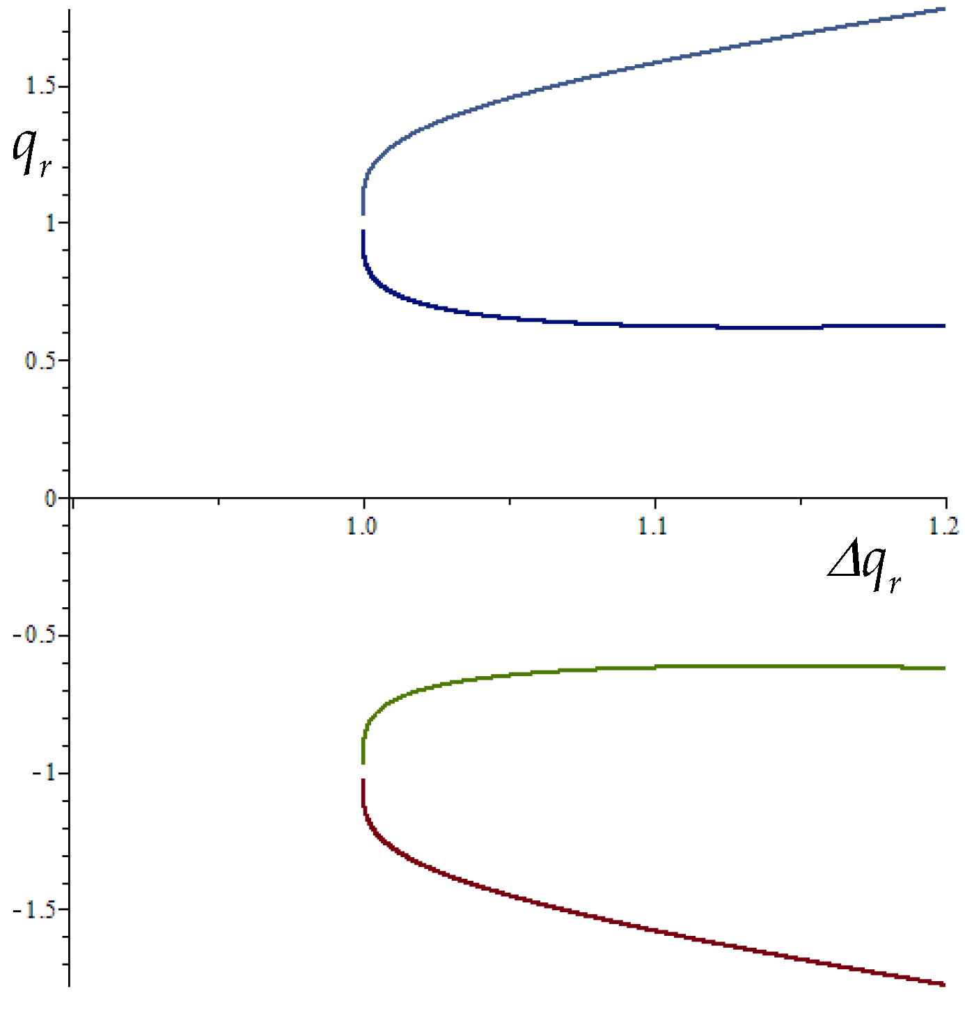
As for the one-layer model, after substituting Equation (64), it is revealed from the imaginary part of
that
. Then, there is only one equation left, which cannot be used for the purpose described above, and the only
that leads to discontinuity is
. If
and
, then it follows from the real part that
Then, for instance, for
, four curves can be plotted as indicated in
Figure 2. This proves that all
identify a discontinuity, starting from a certain value, which can be determined from the stationary point of the two curves that lie closer to the horizontal axis. It is
, where
is the real part of the frequency, named as the
limiting frequency.
However, the condition
is a unique condition that ensures real coefficients to
. It is therefore possible to use the well-established theory for fourth-order polynomials and obtain the previous result in a simpler way. One can assume
. Real
-roots exist in the full region separated by the first branch identifying the zero discriminant. For
and
, the discriminant can be written as a quadratic polynomial for
and cubic for
, so it is easier to present the analytical solution as
Then discontinuities appear along
and
for
and along the full line
for
. In this case, there is no solution for
. For
and
,
the polynomial is of fourth-order for
and cubic for
, so an analytical solution is still possible, but for
would be now simpler. It is not written here due to its length. This identifies
as a function of
. Then discontinuities appear along
and
for
and along the full line
for
. More details in [
31].
For two- and three-layer models, one should proceed according to Equation (64). More specifically, for the two-layer model with and/or and , the real part of the equation to be solved for a given , has only one occurrence of and is a second-order polynomial in . The imaginary part of the equation to be solved can be divided by that is non-zero and then it depends on and , which means that the solution can be obtained analytically. For instance, is expressed from the imaginary part, substituted into the real part, which will still be a quadratic equation for and thus has an analytical solution, which is not presented here due to its considerable length. After solving for , can be evaluated. Then only valid real values should be used and substituted back into Equation (64). Analytical expressions for and/or would be difficult to obtain, but for selected , it is always possible to simplify the equations as described above and obtain valid real solutions from the two equations with real coefficients by predefined procedures in Maple or Matlab. Maple is preferred because of the adaptable numerical precision induced by the chosen number of digits to be considered. Then, for selected , all discontinuity curves can be plotted by exploiting the valid values of and .
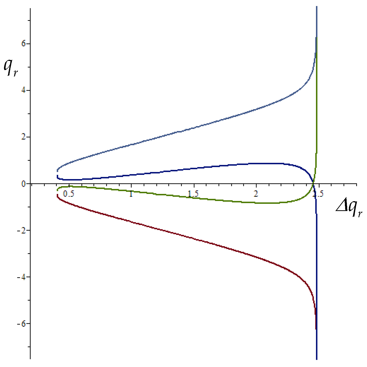
When
, then, similar to the one-layer model, one of the solutions states
. Then, by performing an analysis using only one equation, similarly as presented in
Figure 2,
can be determined from the initial part of the graph. Unfortunately, in this case, there are real
-roots from the very beginning, also for
, thus the
-function is discontinued across
for all
, but the level of discontinuity is negligible until
. This is demonstrated in
Figure 3, from which it can be seen that all
mark discontinuity at
.
One can proceed in exactly the same way with the three-layer model. However, the level of discontinuity for across is negligible only for relatively low , and thus very low .
There are two main objectives of discontinuity lines. First of all, if one would like to calculate exactly the inverse Laplace transform given in Equation (63) by contour integration, branch cuts would have to be introduced to avoid all discontinuities. This can be easily conducted for the one-layer model, but not for the other ones. To obtain some approximation, only the main discontinuities can be considered. Nevertheless, all values at discontinuities are bounded, and as such contour integration is valid. All discontinuities occur for positive and as such the integration along the branch cuts always ceases in time and is never linked to instability. The other aim will be described in the next section.
5.3. Frequency Lines
In some cases, the integral (63) can be determined by contour integration. To do this, it is necessary to determine the poles of the function to be integrated and all its possible discontinuities. The discontinuities are caused by the discontinuities in the
-function, which were discussed in detail in the previous section. As for the poles, one of them is obvious,
, which identifies the steady-state part of the complete solution. The others are roots of the characteristic equation
They are named as mass induced frequencies (MIFs). This name is used because these are not natural frequencies of the model. MIFs are always in pairs, if
is a root then also
* is a root, where * denotes complex conjugate value. MIFs determination is not very easy, because they are complex roots of a complex equation, but three iterative procedures have been described in previous works, [
30,
31]. A good strategy is to start in a region where the convergence of these methods is ensured and then it is possible to follow their evolution as a function of
, which allows for a good estimate of the next value. By connecting these values, one obtains the so-called frequency lines.
After determining the MIFs, then
and thus
The first two terms in Equation (69) can be evaluated semianalytically, which means that the roots of the characteristic equation should be calculated numerically, but all the rest is described by analytical formulas. The last term corresponds to numerical integration. The first term in Equation (69) is the steady-state solution, i.e., the same solution as for the moving force. The sum represented as the second term is called the unsteady harmonic vibration. This is because each pair of forms a harmonic function, which, however, is part of a transient solution, i.e., unsteady. The last term is necessary because it corresponds to the integration along the branch cuts, which must be introduced to avoid -function discontinuities and thus ensure the correct values of the contour integration. Discontinuities in the -function are bounded; therefore, the contour integration is possible and valid.
As for the association with unstable behavior, this is determined by the second term. If there is at least one -pair with a negative imaginary part, then the vibration is unstable, if all pairs have a positive imaginary part, then the unsteady harmonic vibration will cease in time. If at least one pair is real and the others have a positive imaginary part, then the unsteady harmonic vibration will theoretically last forever. The first and the last terms in Equation (69) are never associated with instability. The first term is the steady-state solution (as already written above) and the last term ceases in time, because the discontinuities are always located in the positive imaginary part of the complex -plane.
Since the -function is continuous in the negative imaginary part of the complex -plane, the MIFs indicating instability can always be found by one of the three iterative methods.
However, and especially for the three-layer model, there are several -intervals for which no MIFs exist. The frequency lines are interrupted when the imaginary part of a MIF reaches a discontinuity, therefore, when one strives to obtain MIFs, then in regions with severe discontinuities, where the iterative procedures converge with difficulty, it is advisable to use discontinuity lines which can be easily determined in advance, to identify -intervals without MIFs. In addition, the frequency lines reflect the behavior of the instability lines, which are easier to determine, as will be explained in the next section.
As the discontinuities are always located in the positive imaginary part of the complex -plane, this means that in the negative imaginary part of the complex -plane the -function is continues and thus MIFs indicating instability can always be determined. In other words, -function discontinuities do not interfere with the determination of unstable behavior. There is no need to use the D-decomposition method to establish -intervals for unstable behavior.
5.4. Instability Lines
Instead of following full frequency lines to determine the onset of instability, which means solving the complex characteristic equation for complex roots—MIFs, it is much easier to trace the so-called instability lines, which keep the analysis in the real range. Instability lines are determined in damped scenarios. The -value at the onset of instability is generally indicated by the intersection of the imaginary part of the frequency line with the horizontal axis, that is when the imaginary part of the MIFs is changing sign. Therefore, at such a separation the MIF is real, which in fact still indicates a stable situation. Considering the characteristic equation (67), it is obvious that it is much easier to choose in a particular scenario, find real that gives real -function, and then calculate the corresponding . Such can be efficiently found by a simple bisection method when a change in sign of is detected. There may be several instability lines for the same case.
One can conclude that instability lines cannot end abruptly like frequency lines, they must asymptotically tend to infinity or be closed. An asymptotic tendency of to infinity is detected when either or tend to zero. Additionally, one of the instability lines will have only one asymptote to infinite and the other end will tend to while will tend to infinity. In general, one can start with very low to search for all asymptotes with tending to infinity. Using these values as starting points will allow the lines of instability to be traced using adequate estimates. Then, asymptotes with tending to zero are usually detected at the end of the already started line. After that, it is necessary to check some -values to identify closed instability lines. Their existence is usually revealed while tracing other instability lines, as they will be close together at some point. By careful analysis, one can be sure that the entire -plane is being scanned, which is not the case with frequency lines. After scanning the entire -plane, the -intervals of instability can be determined.
The bisection method can again be used to obtain exact values of and for given from the scenario under consideration. By fixing to a specific value, all intersections can be found. The particular shape of each line then clearly identifies whether each crossing indicates an Onset of Instability (OI), an End of Instability (EI), or merely adds (or removes) one unstable MIF to an already existing one (from at least two already existing ones). Later cases will additionally have the adjective “false”, thus, in the abbreviation FOI and FEI. Specific cases will be shown in the examples section.
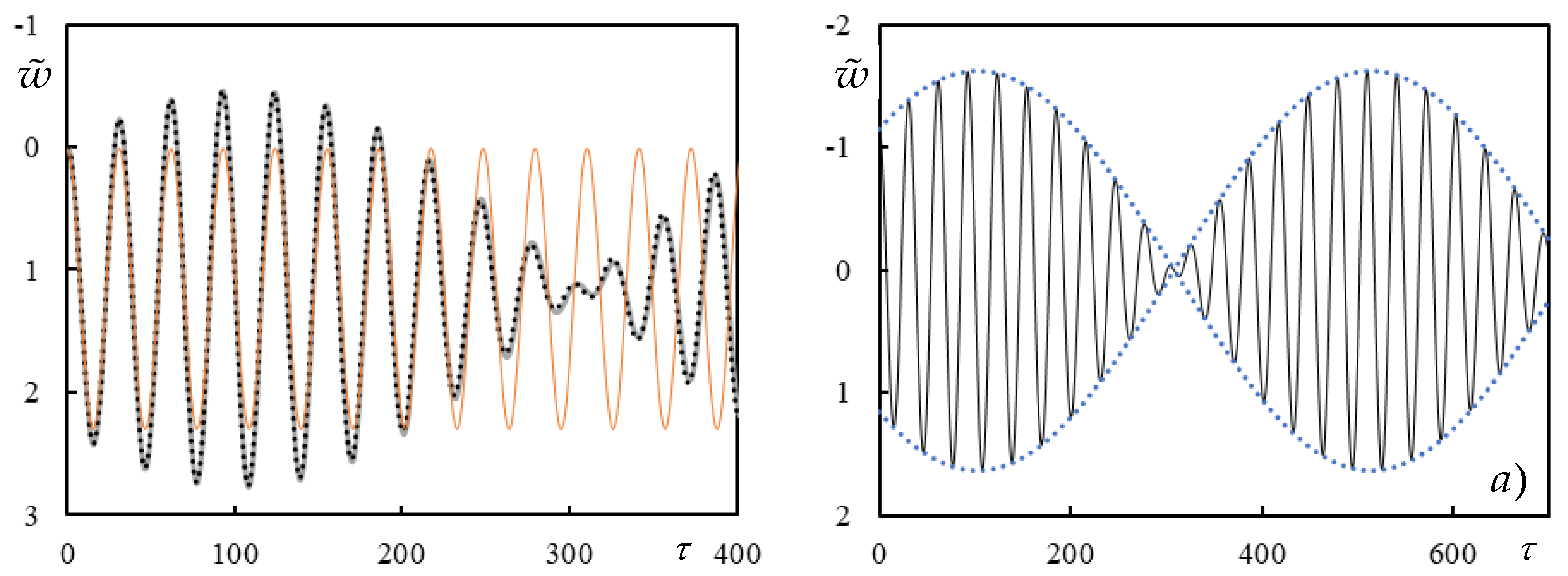
5.5. Time Series of the Active Point
The time series of AP or of any other point along the beam can be determined numerically using Equation (63). Unfortunately, this is the only viable path for the three-layer model. However, for one- and two- layer models very good approximations are obtained by exploiting Equation (69) with neglected . This is because the MIFs of these cases are well-defined and thus the harmonic part of the full solution provides a very good approximation of reality. In such cases, is only noticeable at the very beginning and only in cases where the harmonic part does not well meet the initial homogeneous conditions.
Another possibility is an analysis of long finite models by modal expansion. Further details are in [
30,
31].
6. Examples
6.1. Data Ranges
No significance is attached to any exact deterministic data associated with a particular track, but all parameters are processed over a wide range of possible values. First, allowable ranges of true values are identified to steer the dimensionless counterparts into some reasonable range. However, for demonstration purposes, academic values will also be admitted, especially for , to illustrate better instability lines behavior.
As for the rail, the range of possible values is quite narrow, basically, there are only two guide sets of values for 54E1 and 60E1 rails that specify limits on
and
, bearing in mind that the Young modulus and density of the steel used to make the rails have values that are not very different. There is a very large dispersal in the values regarding the stiffness of the rail pads. This can vary from 20 to 5000 MN/m, [
19]. The sleepers can be wooden or concrete, so the mass range steeps from 80 kg to 320 kg, [
19].
As for the ballast contribution, the stress cone theory can be used to estimate realistic values. Assuming that the effective sleeper length is equal to 1 m [
19], the sleeper spacing varies between 0.54–0.6 m, the sleeper base is 0.25–0.35 m, the ballast height is 0.2–0.6 m and the distribution angle is 30°–50°, then the formulas from [
19] indicate the stiffness coefficient range as 0.96–3.12 m, the shear contribution coefficient range as 0.03–0.5 m and the volume of dynamically activated mass range as 0.082–0.544 m
3. It should be noted that the above-specified coefficients have a dimension that may look strange, but this is because the stiffness coefficients should be multiplied by the Young’s modulus and the results must indicate the linear spring stiffness in N/m. Likewise, the mass coefficient must be multiplied by the ballast density and the result must have the unit of mass i.e., kg. Admitting the ballast Young’s modulus from 50 MPa till 400 MPa, the ballast density of 1200–2600 kg/m
3 and the Poisson ratio in the range of 0.1–0.45, representative ranges of all values characterizing the ballast can be determined.
As regard the ballast height of 0.6 m, it is necessary to note, that this value may (or may not) be associated with the total depth of the granular layers (ballast and subballast) and then it may reach this value. This implies a simplification applied on granular layers, as the angle of distribution will not be exactly the same. Nevertheless, this approach can be considered more accurate than the attribution of the subballast layer to the foundation. For instance, the value of 0.6 m was used as the maximum value in optimization conducted in [
37].
All the data discussed above are presented in
Table 1, but already in their distributed form, with the assumption that the distance between sleepers can vary in the range
. The lower value is taken from [
38] where in fact 0.545 m is specified. The higher value of 0.6 m is the typical value used on European lines. This value is also specified as the maximum value for Indian railways [
39]. According to some other works, the distance can also be higher, for example, 0.711 m is given in [
40] explaining how it is related to the type of sleeper. However, this value was not included in the estimates below, as it refers to steel sleepers, the weight of which lies between wooden and concrete ones and therefore does not apply to extreme values.
Table 1 is complemented by foundation stiffness ranging from 0.22 MN/m
2 [
41] to 1000 MN/m
2 [
42].
Taking into account the dimensionless parameters definition, one can conclude that:
where the lower level of
is taken as zero, because in some works the ballast shear stiffness is omitted. Damping coefficients, have very dispersed values in the literature, so it is more reasonable to directly vary the dimensionless parameters. Layered models cannot implement some other track components such as under sleeper pads, under ballast mats, and others as separate components. However, these components are primarily involved in damping, and as such their influence can be conveniently attributed to the damping ratios. More about such parameters can be found in [
43,
44]. Values from Equation (70) are directly applicable to the two-layer model as well.
Regarding
: first of all, it must be emphasized that in railway applications the moving constant force does not correspond to the weight of the moving unsprung mass. The unsprung mass is the mass that is in direct contact with the rail, which is the mass that is modeled in this paper. If the moving mass were so large that the force would correspond to its weight, it could be up to 10 t, but if only the wheel mass is taken into account, then it is only around 880 kg. It is also possible to add part of the weight of the axle and bogie to the weight of the wheel. Since the value of
varies between 0.3 to 2.67 m
−1, according to
Table 1, then the range for
is 50–494 for 10 t and 4.4–44 for 880 kg. Nevertheless, academic values will also be used to explain in detail the complete behavior of the instability lines.
6.2. Critical Velocity of a Moving Force
As already mentioned, the one-layer model has only one well-specified CV value, given by Equation (29). There is no need to show some results of the parametric analysis. The situation is different for the two-layer model, but it is relatively easy to establish some criteria. For instance, for
by keeping
, there are always three resonant values, which, when ordered identify CV, FCV, and CV. This is demonstrated in
Figure 4 for one particular case, namely
,
and
. For this case three resonances calculated analytically are:
. It is clearly shown that the odd values fulfill all the expected properties when crossing the resonance, namely the sudden jump to zero at the AP and equal values in the absolute sense for the global maxima and minima over the whole beam. The even value indicates FCV, there is also a resonance but not very clear due to the step in
used for the parametric analysis: 0.001. Nevertheless, this value does not meet the expected properties of CV, so it is FCV.
It has already been mentioned that all dimensionless parameters are defined with respect to a reference Winkler beam characterized by
, nevertheless, by separating the second layer in a two-layer model in order to model the same railway line
may have a different value because it models the layers under the ballast. However, the main difference now is in the additional mass of the sleepers. This will significantly lower CV1. In more detail, for this particular case when
, the CV1 distribution is shown in [
12]. It was demonstrated that the values were mostly dependent on
and practically independent of
, especially for
. The highest value of
was obtained for
, independently on
. In addition, it was derived in [
12] that CV1 can be approximated by
which gives reasonable results for
, and it is based on the equivalent stiffness of two springs in series and a lumped mass. This also means that CV1 would be essentially the same in one- and two-layer models if the mass of the sleepers were directly attributed to the rail, as also proposed in [
1], and
. By increasing
even more, the connection between the rail and the sleeper became rigid and the two models are equivalent. However, there is also FCV and CV2 for the two-layer model, which are not present in the one-layer model.
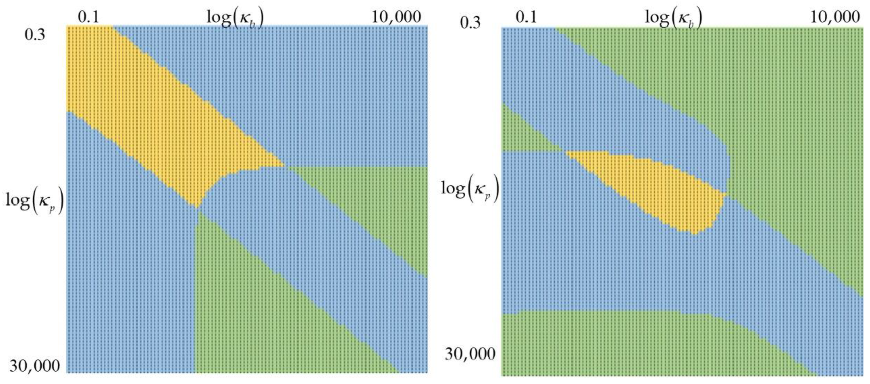
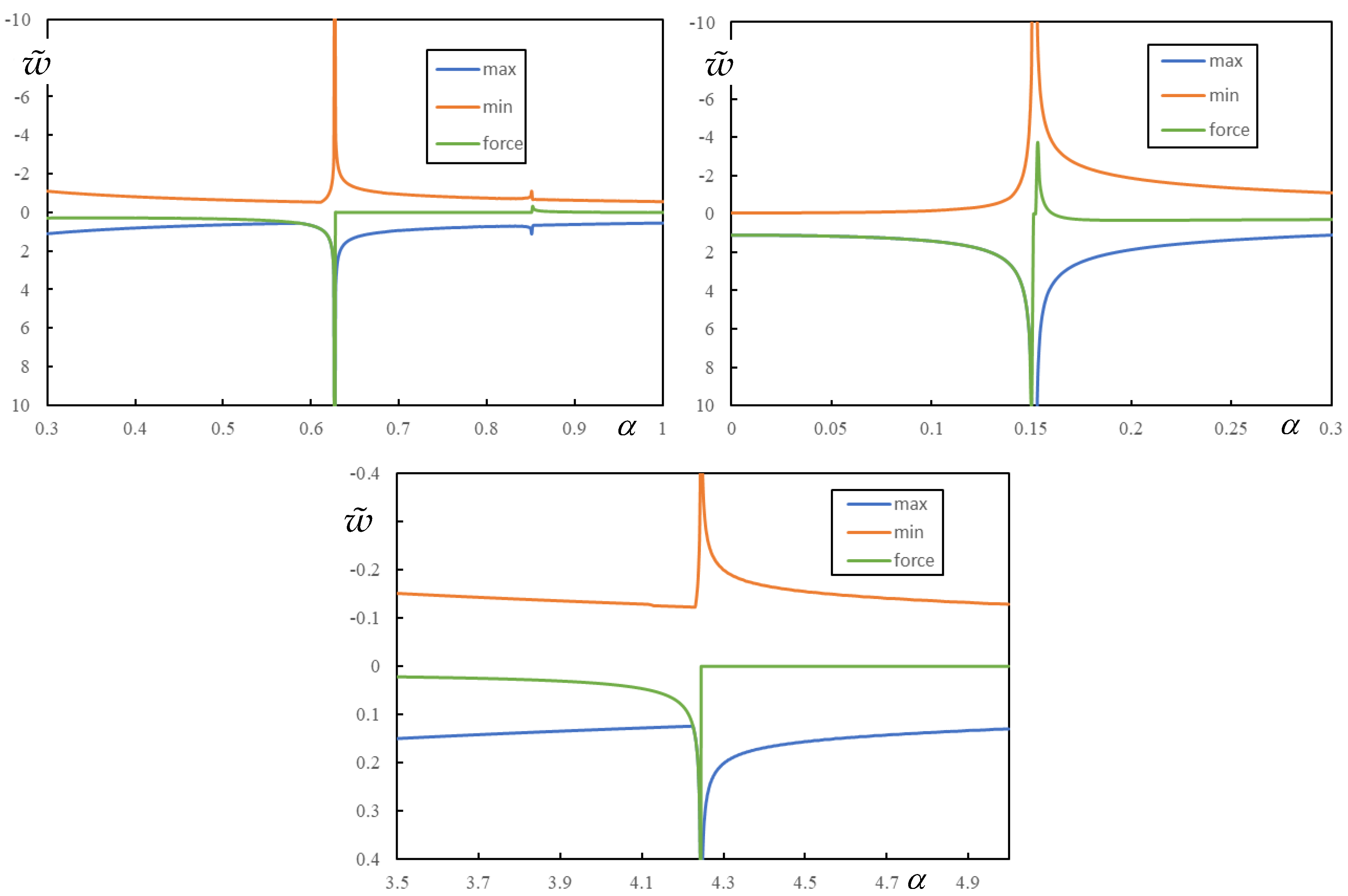
In the three-layer model, the situation is more complicated. Defining parameter regions where there are 1, 3 or 5 resonances is not easy or even possible. This can be conducted parametrically for a specific case, as shown in
Figure 5, for
,
and
; and, for
,
,
and
, with variation of
and
.
It can be concluded from
Figure 5 that no simple general conditions separate the parameter ranges to identify a priori the number of resonances. Several cases are selected to demonstrate what happens if the number of resonances is complete or not. They are illustrated in
Figure 6,
Figure 7, Figures 9 and 10.
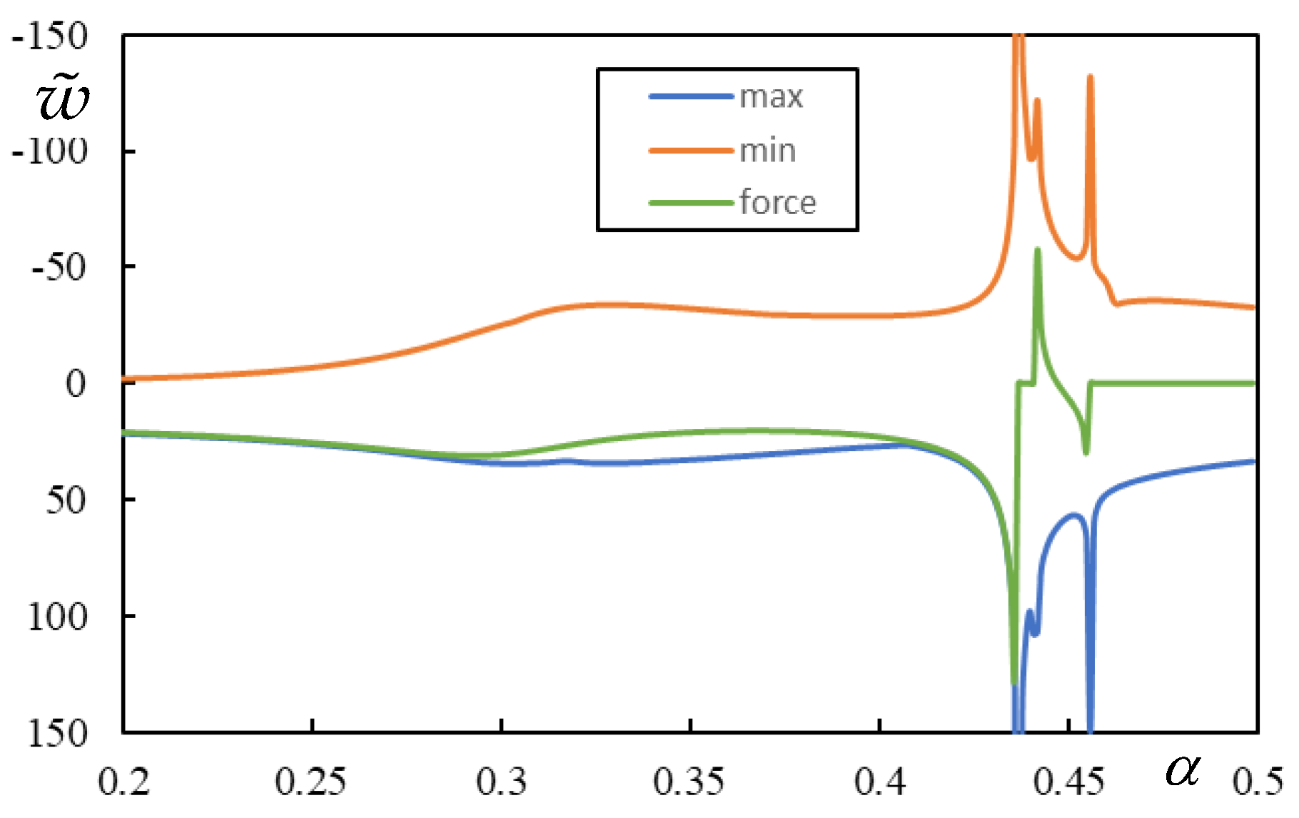
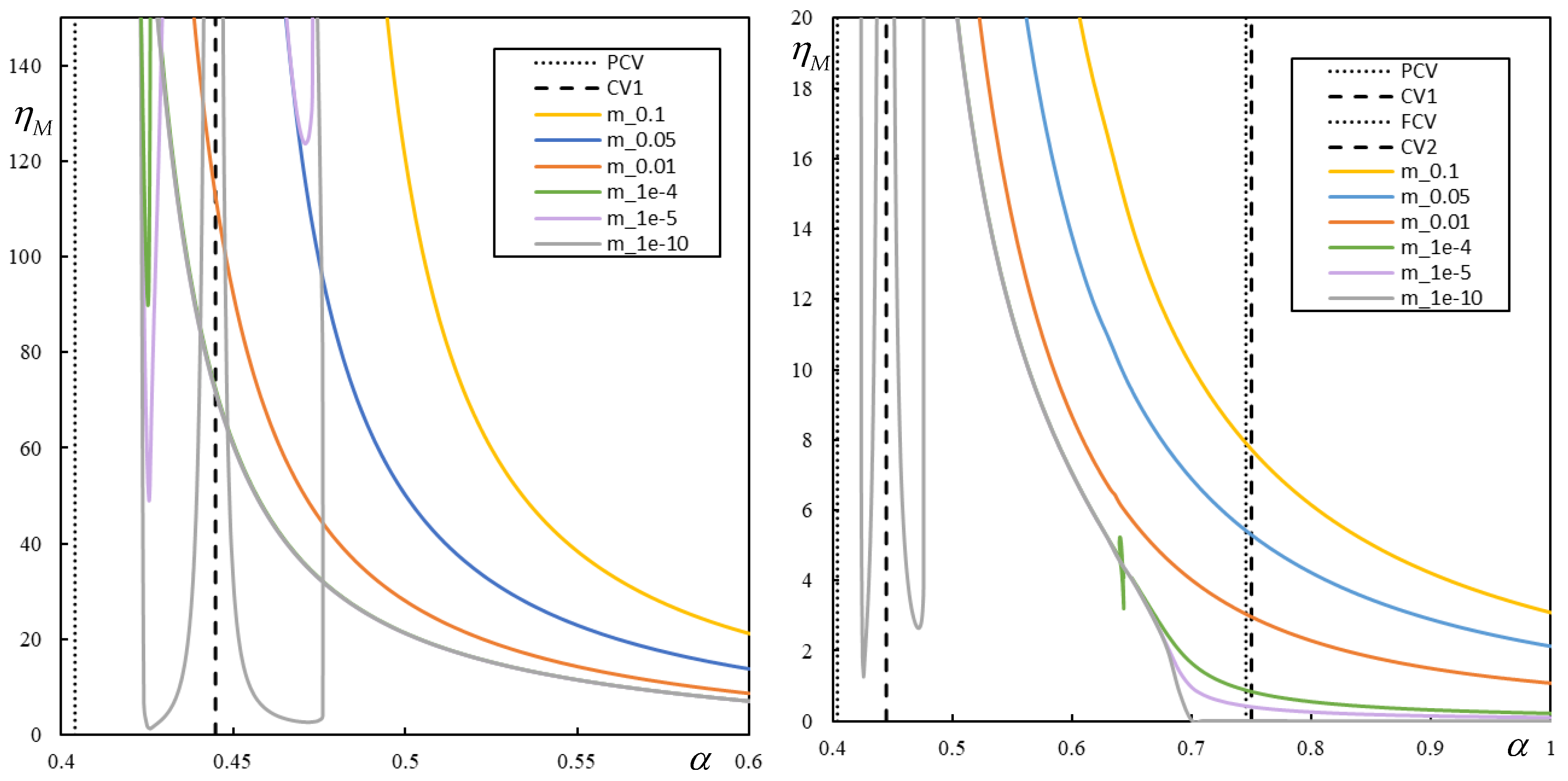
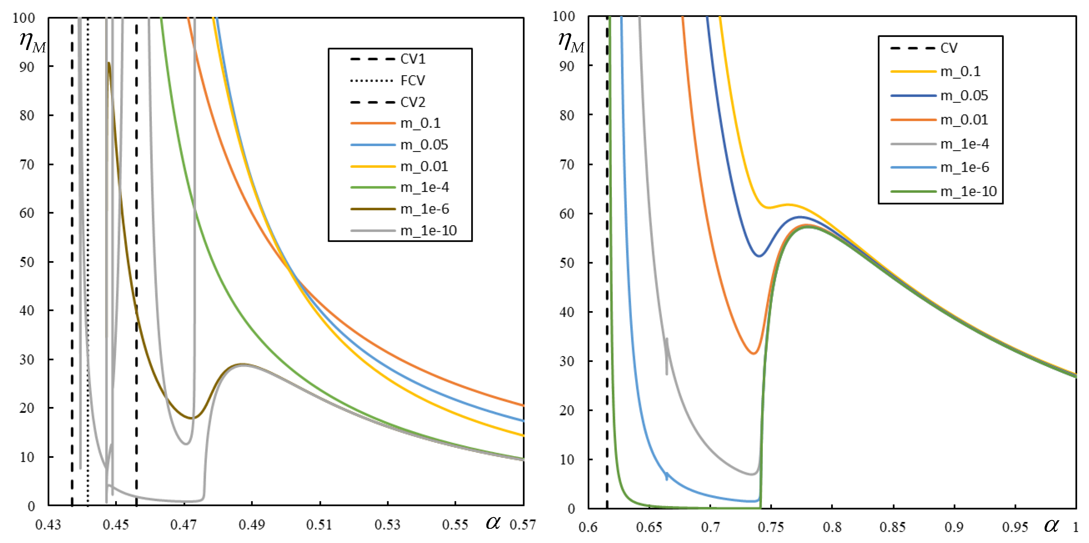
Firstly, in
Figure 6 the case with all five resonances is shown. The case with
,
,
,
and
was selected. Also here, as in
Figure 4, it is demonstrated that the odd values identify CV while the even ones FCV. Resonances determined semianalytically are:
.
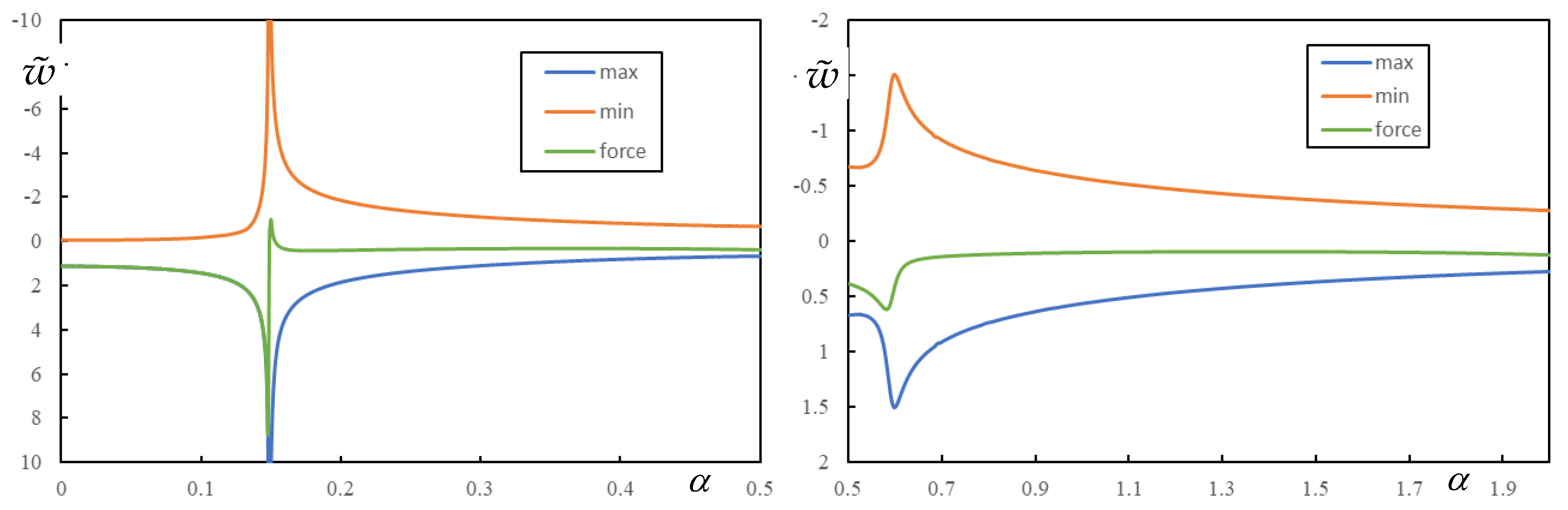
The next case was selected to demonstrate what happens with only one resonance. The parameters are:
,
,
,
and
and the results of the parametric analysis are summarized in
Figure 6. The analytical value is
. Other values are PCV which can be determined only from the parametric analysis. They are 0.149 and 0.599.
From
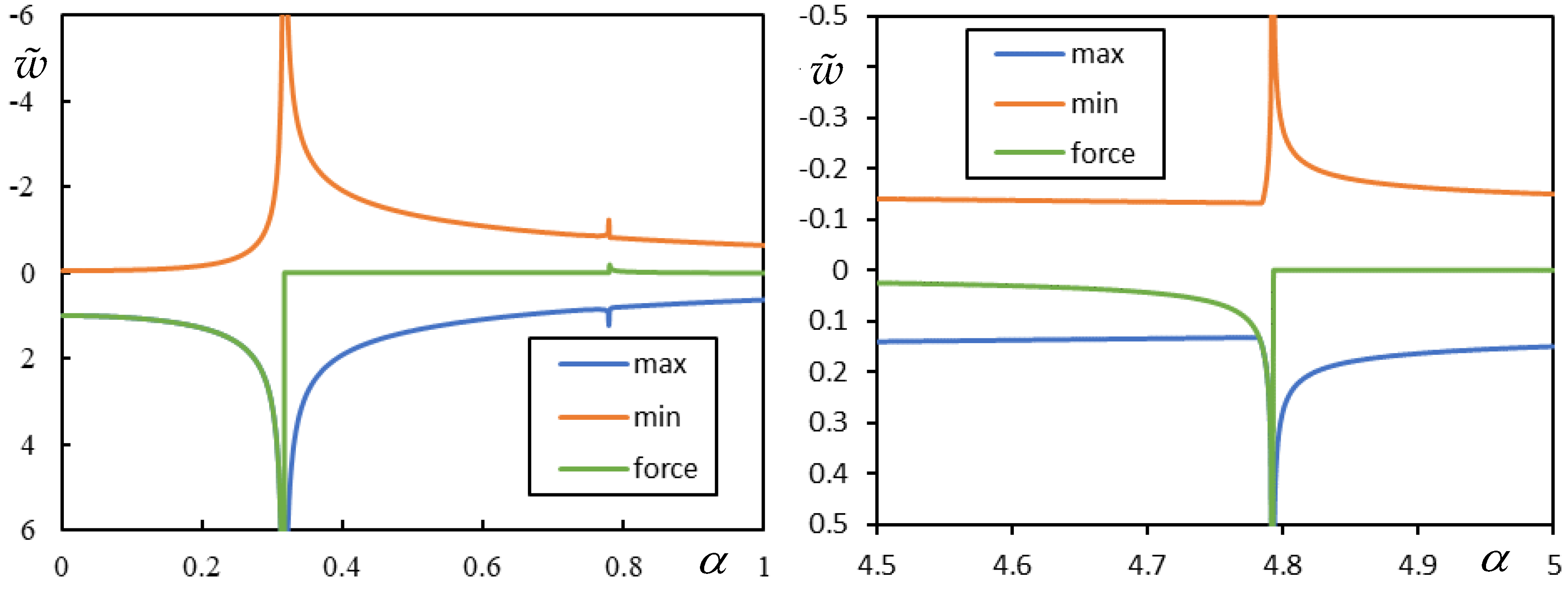
Figure 7, it can be concluded that FCV can only occur between two CVs. When missing CVs are replaced by PCVs, then there are no FCVs between them. It can also be seen that the PCVs can have very different importance depending on the global maxima reached.
The problem with PCVs is that we do not know them a priori, and also that they are a bit imprecise because the three extremes may not be reached for the same value of
. In general, there is no viable procedure other than parametric analysis to find the PCVs position and importance. A single estimate can be based on the “distance” from the region where more resonances occur. At PCV, all extremes are limited, but the augment in deflections can be significant, thus they cannot be ignored. They also play an important role in the analysis of the instability lines. One might think that PCV can be determined in a similar way as CV. CVs are indicated by a real double pole, therefore the polynomial expression as a function of
touches the real axis, so that at the same value the function value and its first derivative are zero. At PCV, the function does not touch the axis, but a first guess would be that the nearest
-value to the real axis would solve this problem. The following
Figure 8 shows that this is not true. Let us analyze the previous case and PCV of 0.599, by analysis of finite beam. If
was CV, then function
would have a local minimum equal to
. By plotting the shifted function
one can find the corresponding value of
. To determine the closest point of the first derivative, one can consider the second one. By solving this the value is different,
.
Using the same philosophy as for the two-layer model, an approximate formula can be proposed for
by
It can be verified that the approximation of CV1 for the case of
Figure 6 is very good, as it gives 0.149. The case in
Figure 7 is also well approximated, but in this case, the value corresponds to PCV1, it is 0.148. This is again due to the fact that the stiffness parameters are relatively high, so the connection with the foundation is stiffer, which allows the use of lumped mass. Thus, the closest value to the one-layer model within the range specified in Equation (70), which means the highest value, can be obtained for
and
. It gives
. Again, by increasing the stiffnesses, masses can be added directly to the beam and the model will be equivalent to the one-layer model.
When stiffness ratios are low, then Equation (72) underestimates CV1 (or PCV1). For example, for the cases in
Figure 9 and
Figure 10 it gives 0.119 and 0.103, respectively. In conclusion, the three-layer model can only approximate the one-layer one when high stiffness and low mass ratios are used. For better correspondence, additional masses should be added directly to the rail in the one-layer model. Low stiffness ratios and high mass ratios significantly reduce CV1 (or PCV1).
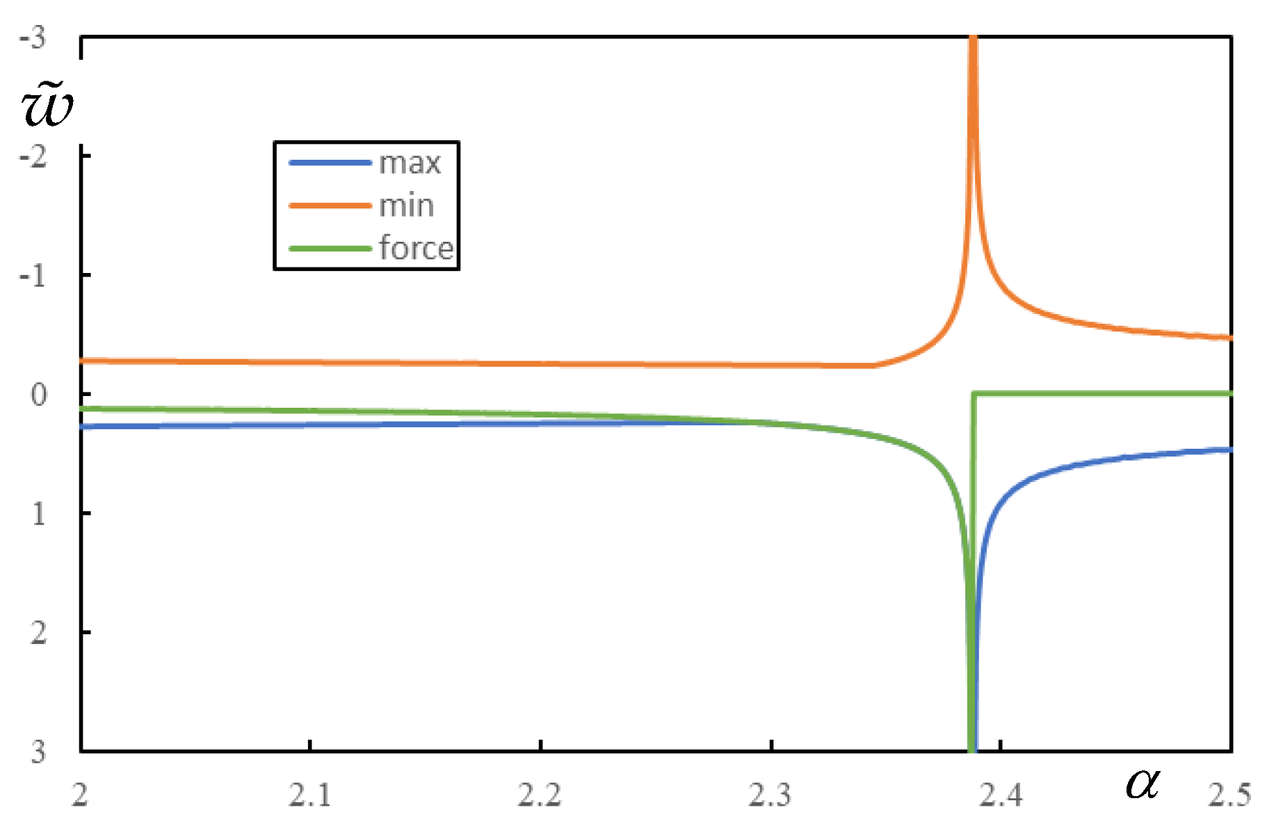
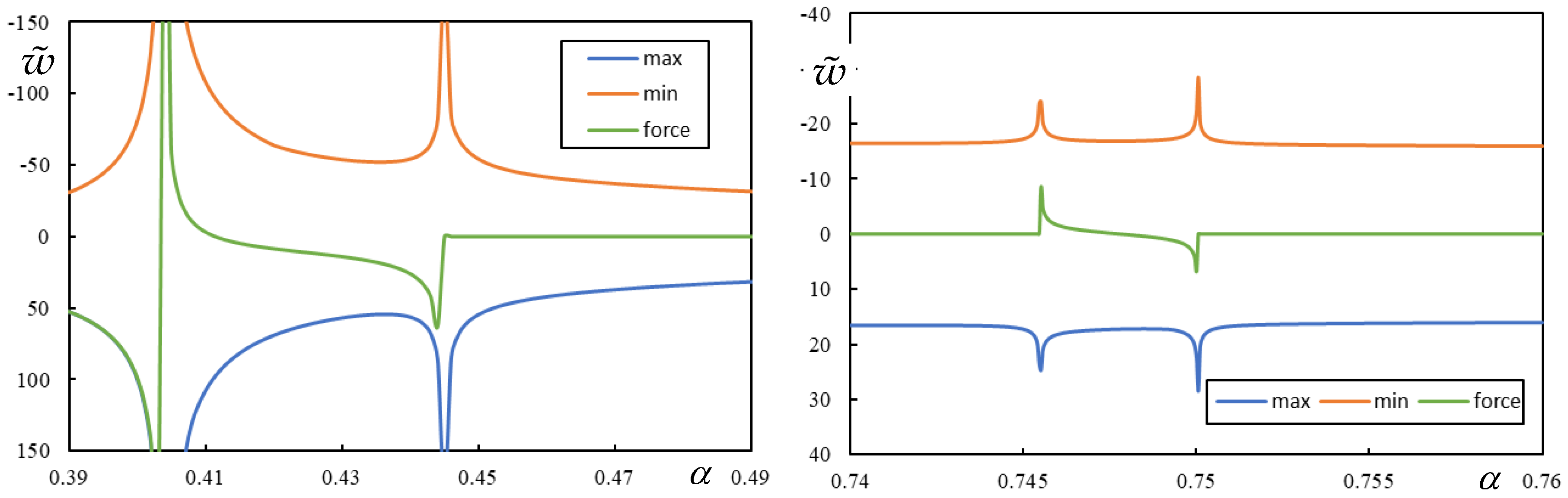
The analytical values for the three resonances are
and
for the case of
Figure 9 and
Figure 10, respectively, the middle value being FCV. In both cases, the lowest values correspond to PCVs, which in the case of
Figure 9 is very dominant and occurs at
, but in the case of
Figure 10 is barely noticeable and its value is not accurate. In both cases, there is no FCV between the PCV and the lower CV, as already mentioned.
The semianalytical approach has three main advantages over the numerical one: (i) in some cases the resonance values can be calculated analytically, if not, then the predefined root determination procedures always provide an exact solution; (ii) if the parametric analysis is used, then this can be conducted without the contribution of damping, as it should, since only without damping the true resonance is detected. The deflection shapes are precisely determined for each tested by contour integration. In the case of real poles, it is safest to introduce some small auxiliary damping to correctly identify the poles describing the deflection before and after the AP. For example, in Maple, a very high accuracy can be used so that when crossing CVs, the deflection at the AP is exactly zero without any rounding, which is able to irreversibly distinguish CV from FCV or PCV; (iii) all values are obtained quickly, accurately and do not need to undergo additional verification.
6.3. Instability of a Moving Mass
The instability lines indicate the separation between stable and unstable , or the separation indicating one more or one less unstable , as a function of . For simplicity, unstable is used to denote at which the motion of the mass is unstable, likewise, unstable means a MIF with a negative imaginary part, which in turn causes the motion of the mass to be unstable. With semianalytical approaches, instability lines can be identified in a simple way without using the D-decomposition method as described earlier.
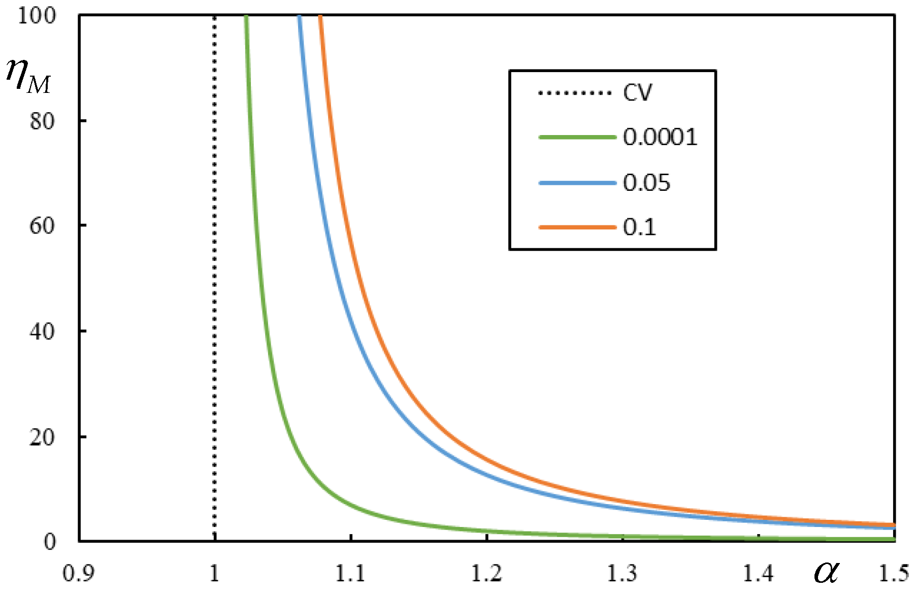
The most regular behavior is identified in the one-layer model. By following the frequency lines, it can be shown that in the undamped case, the CV corresponds to the onset of instability. Under damping, the instability lines have a regular predictable behavior and approach the CV as the damping decreases. This is shown in
Figure 11.
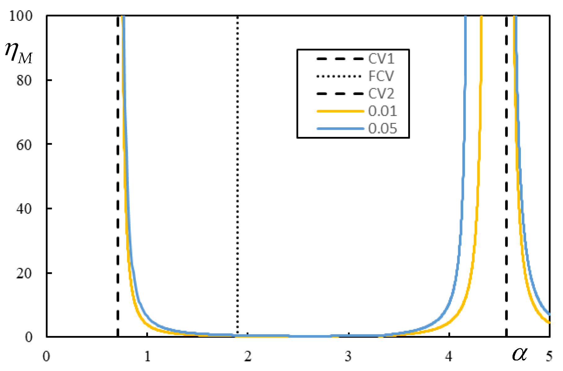
In the two-layer model, a similar regularity can be observed in the case of three resonances. This is shown in
Figure 12. It can be seen that the instability lines are much closer to the critical velocity when approaching from the right than from the left.
It can also be seen that FCV has no effect on the instability lines, again confirming that the usual CV properties cannot be attributed to FCV.
The three-layer model does not provide sufficient regularity as the previous models. Nevertheless, the method described to identify the instability lines is very easy to implement so that full analysis is always possible and gives precise answers. Cases with very low damping can lead to the strange behavior of the instability lines, which will be shown in the further text. Also, the role of CVs and PCVs is not clearly evidenced, and thus general conclusions are difficult to draw. It is shown that there are several such lines. They can have quite a strange evolution, since they can form a closed curve, but they usually end up with asymptotes tending to infinite mass ratio at a fixed velocity ratio, and always one of them is tending to zero mass ratio at infinite velocity. It is also shown that the expected relation to the critical velocity of the moving force is not confirmed. First, three values of this critical velocity do not always exist. Sometimes there is only one, then the others are compensated by pseudocritical velocities, which may or may not be dominant, affecting their influence on instability lines. Second, especially for low damping levels, there are more than five asymptotes at fixed velocity ratios, so they cannot correspond to the three possible vertical lines.
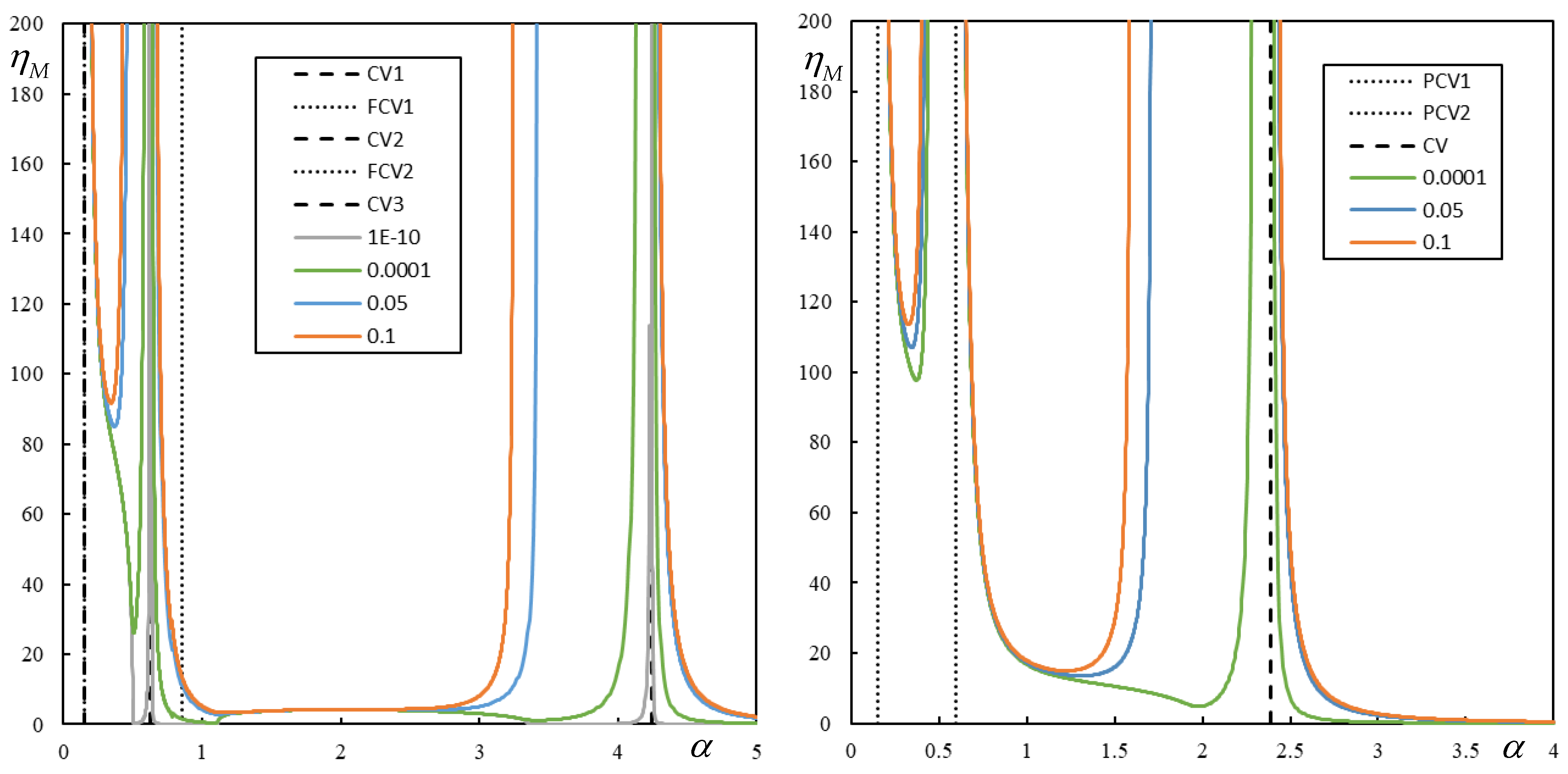
It can be stated that the cases presented in
Figure 13 are quite regular with the expected behavior. PCVs take over the role of CVs, while FCVs have no effect on instability lines as before.
More details about the lastly shown case are now given. It can be seen from
Figure 15 that when the damping levels are high, the instability lines are regular. For low damping levels, like
,
or
, there are several instability lines, but not all of them are visualized in the figure due to its scale. By detailed analysis, nine asymptotes tending to infinity are found for these cases, as indicated in
Table 2, which summarizes the corresponding
of such asymptotes.
To recall, in the case shown in
Table 2 the two CVs are 0.43695; 0.45594 and FCV is 0.44158. As expected, the CVs are approached by the asymptotes as indicate values in the third and seventh column (excluding from this count the indication of the level of damping), but there is no further a priori indication of the other asymptotes. Moreover, the instability lines cross the CVs straight lines, which is also not expected. The PCV is barely noticeable, but certainly occurs for lower
than the first asymptote, as seen in
Figure 9.
As regard instability, then for
and
there are only three crossings, but for
there are nine crossings for
as well as for
. This high number is due to one instability line being closed and strangely shaped. The exact values of
where it happened are listed in
Table 3. Also given in this table is the corresponding
, which is actually the real part of the MIF with zero imaginary part, i.e., it is directly equal to this MIF.
It can therefore be stated that it is very difficult to establish any general conclusions as for a one-layer model or a two-layer model with three resonances. However, the analysis of instability lines is very simple, it is conducted essentially in the real domain, and it is guaranteed that all instability lines are correctly traced, unlike using the D-decomposition method, which requires more sophisticated calculations to obtain each value.
Nevertheless, having the instability intervals also means that all crossings of the imaginary part of the frequency lines are determined. This serves as an indication for further estimations and makes it easier to follow the frequency lines. For low damping levels, then, there are basically two lines that are interrupted at some regions, but their real parts are very similar, and their imaginary parts are approximately opposite, except for the low until the first OI. Additionally, the shape of the instability lines also indicates the shape of the frequency lines.
Previous figures have shown that the onset of instability of one moving mass is strongly related to CV1 or PCV1, whichever is lower. Therefore, the conclusions drawn about models’ differences and the effects of various parameters for the critical velocity of moving force apply here as well.
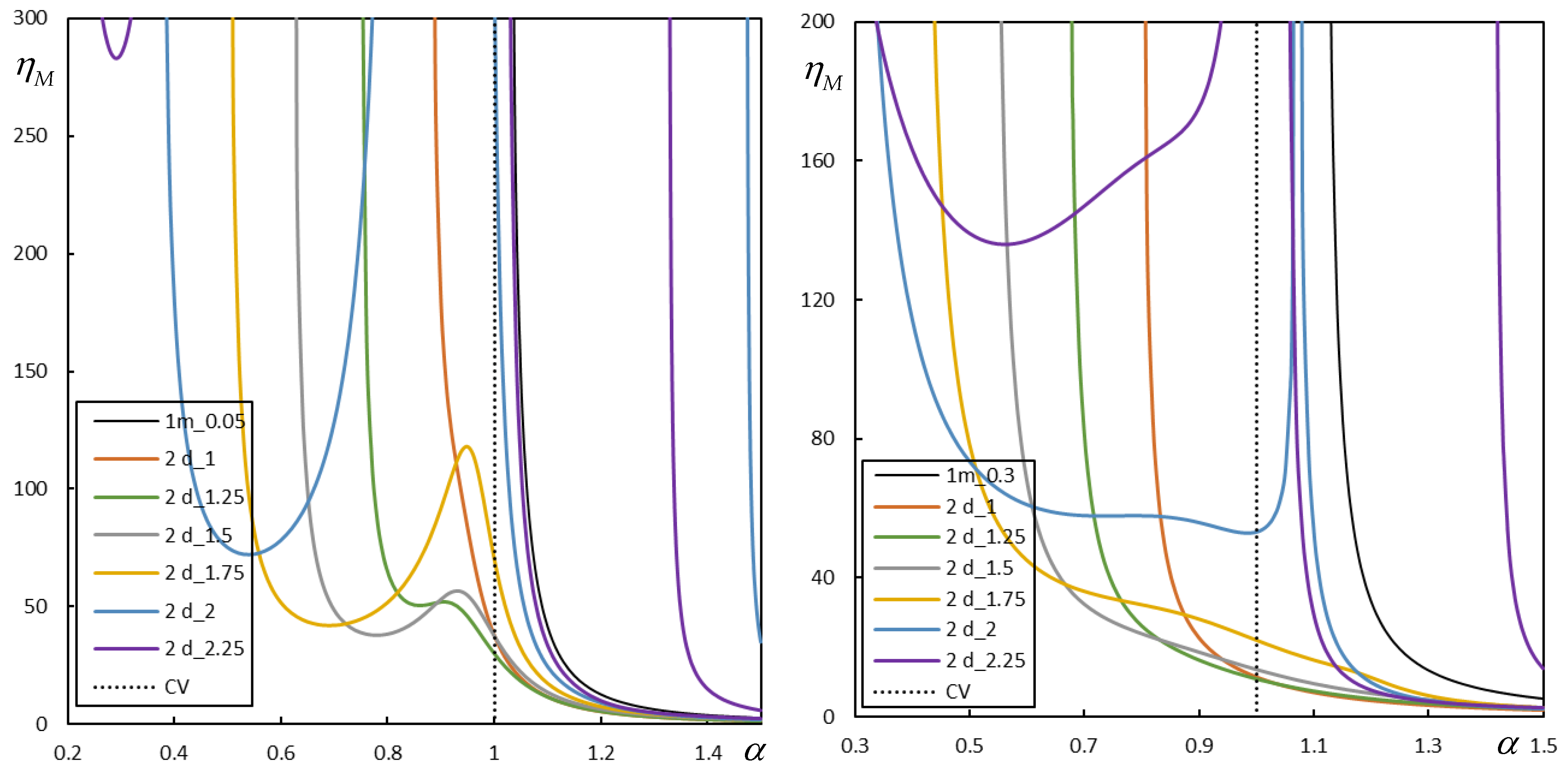
6.4. Instability of Proximate Moving Masses
The last part of this contribution is devoted to the instability of moving proximate masses. This research still needs further attention because, as shown in the previous section, the motion of a single mass on a three-layer model is already quite complicated. For the one-layer and two-layer models, some results have already been presented in [
11,
12], where it was assumed that both masses have the same values and the forces acting on them were also the same. It has been found that there are cases where damping can move the onset of instability to lower
than when only one mass is moving. Moreover, this situation is worsened by increasing damping, rather than improved, as is generally attributed to damping. Some cases are shown in
Figure 16 and
Figure 17. These figures illustrate the instability lines that can be determined in the same way as for a single moving mass, only the characteristic equation is more extensive and has the same form for all three models
where
stands for the dimensionless distance between masses.
Another important fact is that the superposition of the results is generally not possible, and the dynamical interaction is active up to quite large distances between the masses.
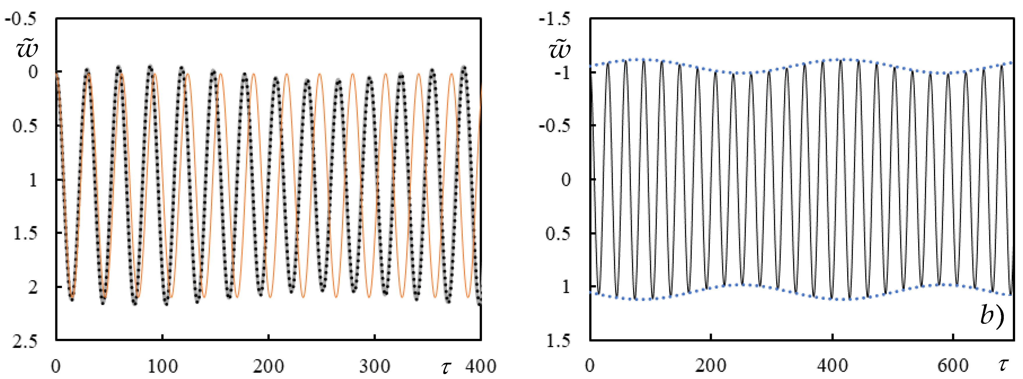
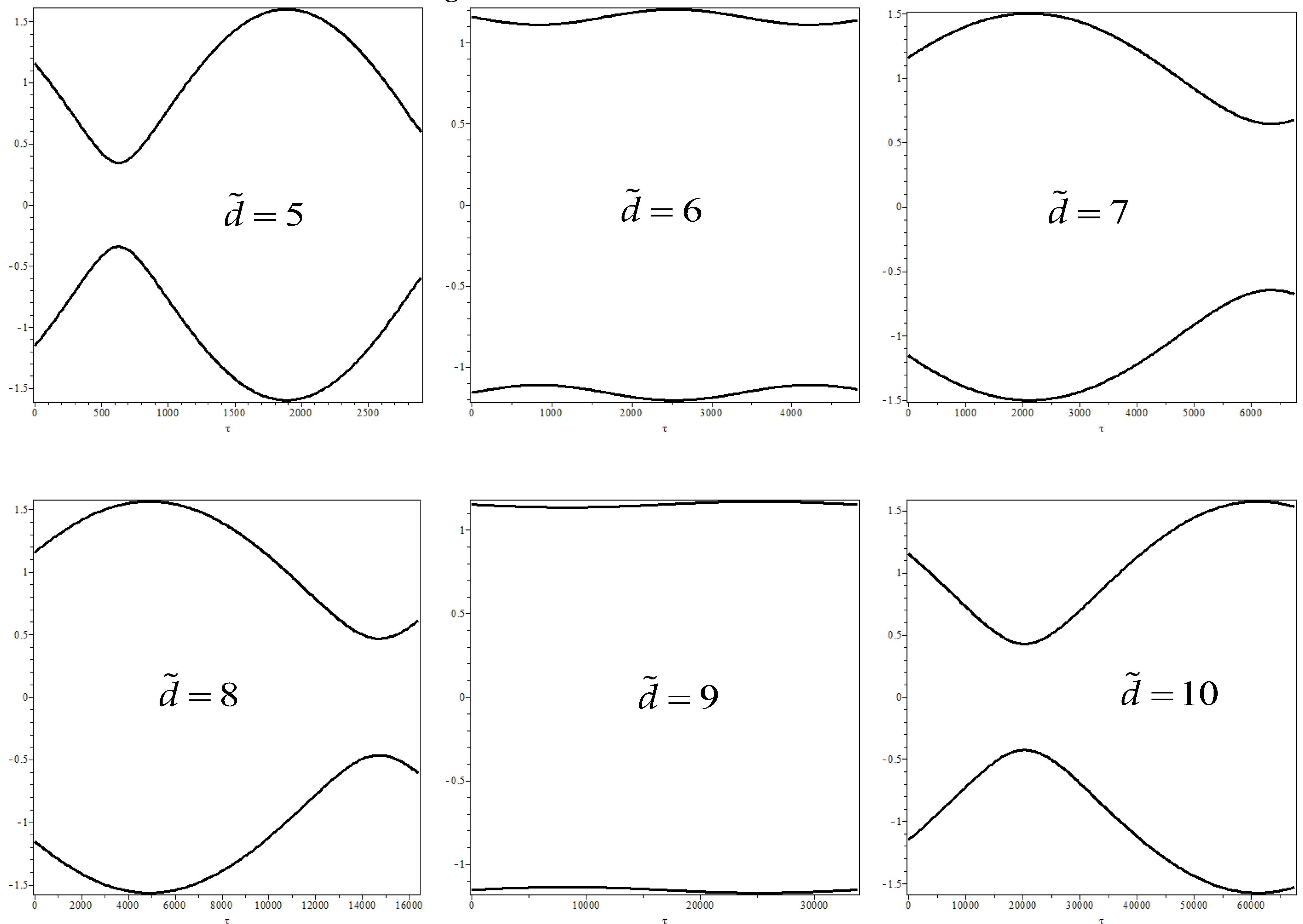
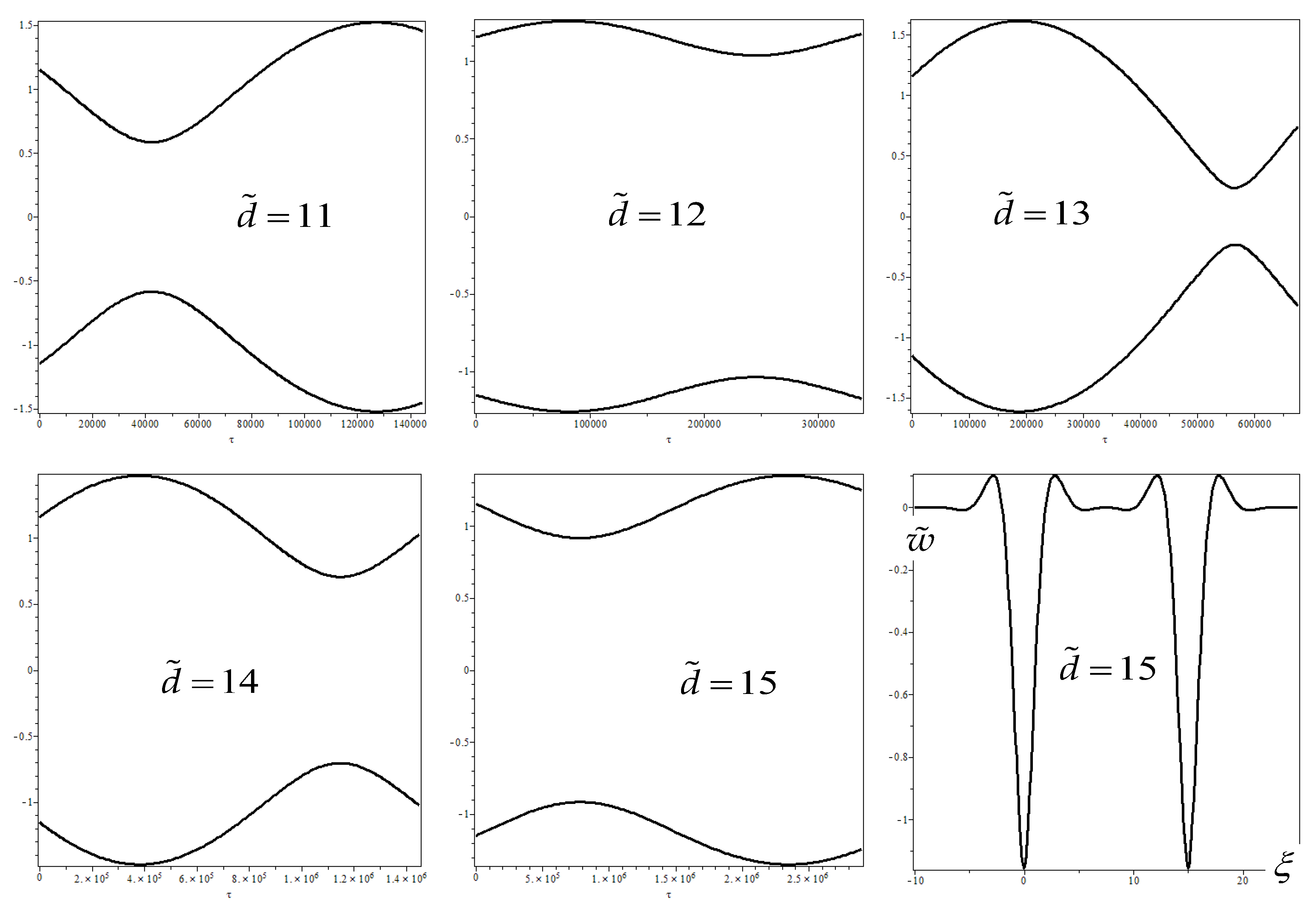
Figure 18 shows the case with gradually increasing distances. This is more severe in the absence of damping because the dynamic interaction is active in the transient part of the full solution.
In
Figure 19, it is seen that the dynamic interaction is still active when the masses are quite apart. Results superposition is not possible as this would imply no amplitudes variation in the unsteady harmonic part of the full solution. Regarding the last case shown, which is for
, the steady-state solution is also presented in the same figure with the deflection along the beam to illustrate the distance between masses.
7. Conclusions
All the semianalytical results presented in this paper were shown to be supported by the exact evaluation of the -function value. This was achieved by a precise contour integration method. In the case of real poles, a simple way to deal with them is to introduce very light damping to distinguish those that should belong to the upper part of the complex plane and vice versa.
It was also seen that damping-free calculations are essential, and this is generally well possible only with semianalytical methods. Numerical methods usually need some damping for numerical stability. For example, the calculation of critical velocities using parametric analysis would not be accurate because it would be difficult to distinguish the dominant PCV from the CV.
Regarding the critical velocity of the moving force, it was shown that when the models are compared to a reference Winkler beam, i.e., the one-layer model without shear resistance and axial force, then the other models have CV1 or PCV1 (whichever is lower) always lower. It can never reach the one-layer model value, in this case 1. It can only be attained from below when high stiffness ratio(s) and low mass ratio(s) are used.
However, the three models also differ in the number of layers, and each layer includes additional CV or PCV and sometimes FCV as well.
As for the lowest velocity ratio indicating the onset of instability of a single moving mass, only the one-layer model is fully regular. Instability occurs at CV in the absence of damping, and it moves further away from CV with increasing damping and decreasing moving mass ratio. The interval of unstable velocities always ends at plus infinity, there are no closed intervals of instability. A similar regularity can be observed in the other models only when higher stiffness ratio(s) are used. However, this regularity is always affected by additional CVs or PCVs that form the vertical asymptotes of the instability lines. When using a low stiffness ratio(s), this regularity is violated and vertical lines of CVs and PCVs can be crossed by instability lines. Moreover, with decreasing damping additional instability lines are formed, implying more than one instability interval of velocity ratios and the occurrence of FOI and FEI.
When considering two moving proximate masses, the regularity is violated even in the one-layer model and the same behavior is detected in the two-layer model and low mass ratio. It is expected that irregular behavior will also be present in the three-layer model, but this will be the subject of further research.
It is of note that FCV has no effect on instability, nevertheless, one must be aware that there is no steady-state solution for FCV and as such no solution for moving mass or masses.


