1. Introduction
Resonance-induced vibrations are a major cause of concern and a rigid limiting factor in the design and operation of many technological systems [
1]. Consequently, substantial research effort has been channelled in this direction, leading to several passive and active resonance-damping techniques being reported [
2,
3,
4]. Due to their superior performance, high-tunability and robust performance under parameter uncertainties, active closed–loop damping schemes have been favoured over their passive open–loop counterparts [
5,
6]. Integral Force Feedback, Integral Resonant Control, Velocity feedback, Active Shunt damping, Resonant controllers and Robust Control have all been reported to deliver excellent damping performance [
7,
8,
9,
10,
11,
12]. All these controllers are implemented in the standard negative feedback.
Another family of second–order damping controllers that are typically implemented in a positive feedback configuration are also equally popular. This group consists of the Positive Position Feedback (PPF), the Positive Velocity Position Feedback (PVPF) and Positive Acceleration Velocity Position Feedback (PAVPF) [
13,
14,
15,
16]. Successful application of these Positive Feedback Controllers (PFCs) is well-documented throughout relevant literature. These controllers have been employed predominantly to damp system resonances where a lightly-damped resonant mode at relatively low frequencies (≤1
) dominates the overall dynamics, and the higher–frequency modes are sufficiently far away from the first mode. Examples of such systems are piezoelectric–tube nanopositioners, nanopositioning platforms, high–density memory storage devices, aerospace structures, flexible manipulators, cantilever beams, civil structures, disc drive actuators, etc. [
17,
18,
19,
20,
21].
Though these PFCs are popular and show adequate robustness under parameter uncertainties, their design is based on pole–placement via trial–and–error. As such, a systematic design strategy or optimisation of the controller design against certain application–specific indices has remained elusive. Consequently, the selection of closed–loop pole locations that deliver optimum damping performance has proved difficult. It is also noticed in several cases that increased damping comes at the cost of increased closed–loop DC sensitivity. In many applications such as precision micro– and nanopositioning, increased DC sensitivity is undesirable but inherently unavoidable if PFCs are employed for damping [
22]. Consequently, a systematic method of optimising these popular pole–placement–based PFCs has the potential to positively impact a wide range of technological systems.
In this work, all second–order PFCs, namely the PPF, PVPF and PAVPF controllers, are parametrically analysed for maximising closed–loop damping with respect to closed–loop DC sensitivity (DC gain), thereby allowing for the selection of an optimal solution that satisfies the combination of the aforementioned. It is crucial to note that DC sensitivity and DC gain are synonyms for each other in this context. If the DC gain increases, the sensitivity to low–frequency noise thereby increases, thus affecting system performance. Conversely, if the DC gain decreases, then attenuation of all frequencies occurs, which thereby attenuates the desired output from said system. It is crucial to highlight in this work that when the phrase “DC sensitivity is minimised” is used, it is akin to saying that the “DC gain is brought as close to zero as possible”.
In addition, each PFC is put in closed–loop with an integral tracking controller and optimised with respect to controller bandwidth using the point. A method of systematically designing any of the three second–order positive feedback controllers for optimum performance in terms of closed–loop damping achieved and closed–loop DC sensitivity is presented. The novelty in this paper consists of the following;
Full parametric analysis of the PFC family,
Inform the selection of an optimal solution for each of these controllers with respect to maximising closed–loop damping and keeping the DC gain as close to zero (minimising DC sensitivity) simultaneously,
The analysis and design of an optimal tracking controller for each type of controller for combined tracking and damping applications in which tracking bandwidth is maximised,
Definitive guidelines for the selection of positive feedback controllers for damping, as well as combined damping and tracking applications.
The paper is constructed as follows;
Section 2 introduces the open–loop system and then details the closed–loop equations for PAVPF control, which leads to the matrix equations involved with optimal gain selection,
Section 4 details the optimisation of PPF with detailed closed–loop results,
Section 5 details the optimisation of PVPF with detailed closed–loop results,
Section 6 details the optimisation of PAVPF when designed in a mathematically overdetermined manner,
Section 7 details the optimisation of PAVPF in a mathematically determined manner and draws conclusions compared to the prior mentioned, and lastly,
Section 8 draws important remarks and conclusions about the controller family as a whole.
2. Preliminaries
In general, systems such as nanopositioners, flexible robotic manipulators, sensors and disc drives can are collocated by nature and can be generally modelled by a series of infinite second–order resonant transfer functions as follows:
where
is the DC gain,
is the damping ratio and
is the resonant frequency of the ith resonant modes, respectively, such that
. To simplify the system, it is important to note that the first resonant mode is dominant and usually separated far away from the higher resonant modes [
23,
24]. It has also been noted that if left undamped, this highly-dominant first resonant mode enforces severe limitations on the operational safety, as well as positioning performance of the aforementioned systems. Consequently, most techniques focus on damping this first resonant mode, and subsequent controller designs are based on a plant model, consisting of a second–order transfer-function (accounting for the dominant resonant mode) [
25] and an adequate feed–through term (accounting for the truncation of the higher–order dynamics) [
26]. The simplification for (
1) is as follows:
where
,
and
are the first resonant mode numerator constant, resonant frequency, damping ratio, respectively, and
is the feed–through term, which accounts for truncation effects. In order to dampen the dominant resonant mode of such systems, a family of positive feedback controllers have been developed, namely PPF (Positive Position Feedback) [
27], PVPF (Positive Velocity Position Feedback) [
22], PAVPF (Positive Acceleration Velocity Position Feedback) [
16] and IRC (Integral Resonant Control) [
23]. In this work, the primary focus is the positive feedback controller consisting of PPF through to PAVPF. Consider the following definition for PAVPF control;
where
are controller gains to be determined. To derive the PPF and PVPF controllers, all that is required is to set
and
and
to zero, respectively, for the controller of interest in Equation (
3);
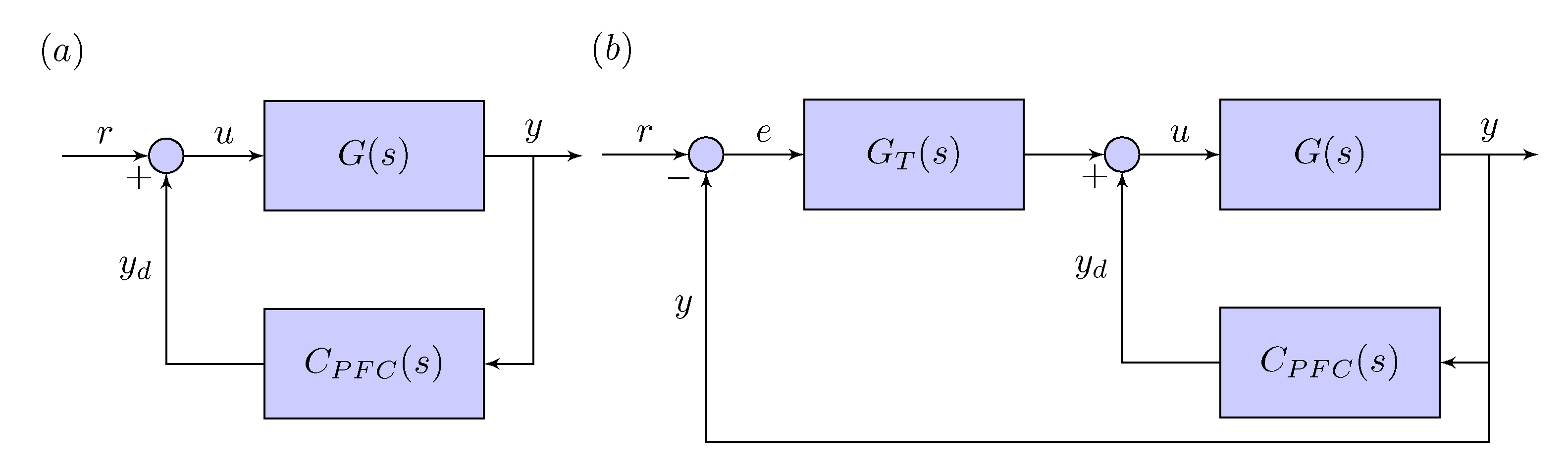
Figure 1 shows the general closed–loop configuration structure for damping (
a) and damping with tracking (
b) respectively. Since this family of controllers are damping–focused, the central design criteria are to bring the closed–loop damping as close to one as possible. To this end, the most important gains to optimise are
,
and
, respectively. A secondary but equally important performance index to consider is the DC sensitivity. It is most desirable to impart maximum damping to the resonant mode without forcing any change to the overall system’s DC sensitivity. Though this has remained elusive in most positive feedback implementations documented in the relevant literature, this exercise aims at categorically proving that such a design cannot be achieved in the PPF case and proposes designs for PVPF as well as PAVPF where both performance indices (high damping coefficient and unchanged DC sensitivity) are adequately met. Consider putting Equation (
3) in positive feedback with Equation (
2):
The closed–loop equation can be summarised as:
where the denominator and numerator coefficients are shown in
Table 1 and
Table 2.
From this point, the ideal pole–placement methodology is discussed and demonstrated. Consider an ideal fourth–order, the closed–loop system whose poles are given by:
These repeated poles are chosen such that their damping is identical, which allows for easy computation and easy comparison with actual imparted closed–loop damping. Then the desired characteristic polynomial
that has the roots given by Equation (
8) is defined as:
In order to perform pole–placement between the desired polynomial (
9) and the coefficients defined in
Table 1, they are set equal to one another as follows;
To this end, the denominator coefficients seen in
Table 1 are rewritten in terms of a system of matrix equations. The method is based on nonlinear optimisation, in which a sophisticated objective function, as seen in Equation (
16), is comprised of Equations (
14) and (
15). It should be noted that the objective function originates from matrixial representation (
12) of the characteristic polynomial in a closed–loop system. A vector of the controller variables,
is formed, and then the system of equations corresponding to this isolated vector is formed as follows;
or more compactly:
such that
and
. Since the desired pole locations are set through the coefficients of the desired characteristic polynomial (
9) as defined in (
11), this means that the only set of unknowns is that of the controller variable vector
in the system of Equation (
12). This numerically implies for a specific
set that solving this system of matrices yields the optimal
vector for all other controller variables, not including
. As a result, to optimise the controller in the case of PAVPF, a simple numerical sweep for
, combined with solving this system of matrices for each
chosen, will yield the optimal set of gains based on the performance metrics chosen, namely; maximising closed–loop damping while keeping DC sensitivity minimal or rather keeping the DC gain as close to zero as possible. More specifically, if the closed–loop damping ratio is computed from Equation (
8) as:
and the DC gain can be computed by the following:
As a result of requiring a numerical search, the controller vector
becomes a function of the real part of the poles as well as the
chosen. The overall optimisation goal for damping applications can be summarised as follows:
In the following sections to come, the matrix system of Equation (
12) and the desired characteristic polynomial (
9) provide the basis for the optimisation of all respective controllers. The next subsection details the optimisation procedure for applying integral tracking to PAVPF control and hence PVPF and PPF, respectively.
Integral Tracking Optimisation
Within the context of optimising for both combined damping and tracking applications, the primary optimisation goal is that of maximising the controller bandwidth, namely the
dB point. To incorporate tracking control to the closed–loop system described by Equation (
7), firstly consider the following basic integrator with gain
K:
The new closed–loop equation with integral tracking can be derived by applying Equation (
7) in negative feedback with Equation (
17) as follows:
In order to optimise damping and maximise control bandwidth, the integral gain
K needs to be optimised such that both of these factors are considered simultaneously. To this end, it is required that:
This ensures that for no possible frequency
, the closed–loop system response exceeds that of
dB, ensuring maximum damping, as well as maximising the
dB bandwidth of the closed–loop system, which ensures better tracking performance. To optimise
K,
must be derived. Begin by substituting
into (
18), gathering real and imaginary terms, which results in:
then computing
:
by using the inequality presented in (
19), expanding (
21) results in a 10th–order polynomial in
as follows:
where the coefficients can be seen as follows in
Table 3 and
Table 4 respectively.
Rearranging (
22) results in the following polynomial, which is a function of
and
K:
noting that
cancels out, thus reducing to the following polynomial:
letting
, this results in the final optimisation polynomial:
In order to yield the optimal
K from Equation (
25), the optimisation problem requires an important selection of
to yield the correct quadratic equation in
K. The correct selection of
is achieved by finding the frequency of the dominant resonant poles of the controlled system and the damping ratio of the controlled system in question. Once these are found, they can be substituted into Equation (
25), which will yield the correction optimisation problem for
K and, hence, the correct choice of
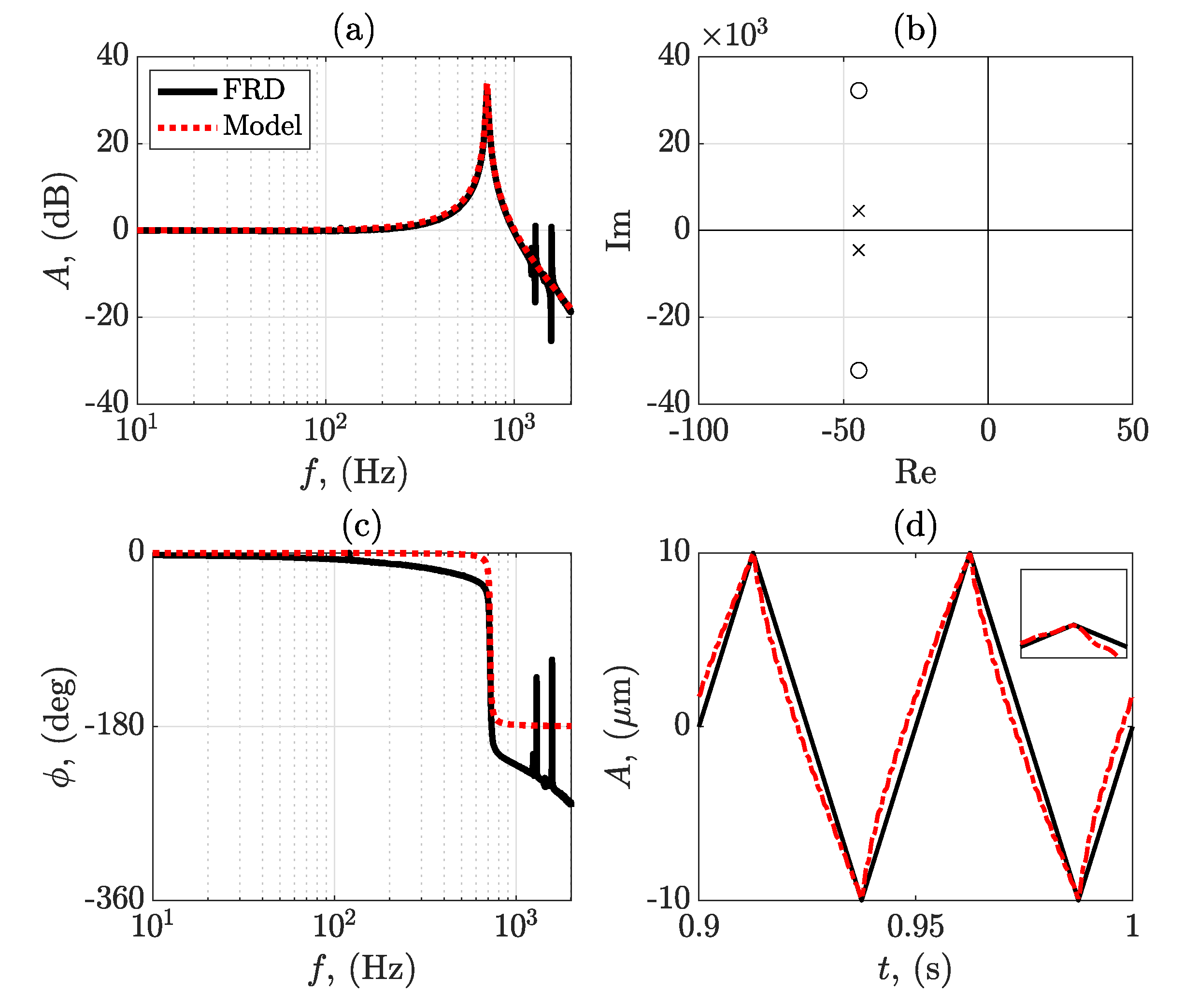
K. This will be shown in detail for each controller type in this paper. Moreover, in the following section, the open–loop system is generated from experimentally sourced frequency response data based on the nanopositioner system at the University of Aberdeen [
16].
4. PPF Optimisation and Analysis
To begin with optimising PPF control, the matrix system of Equation (
12) needs to be reduced accordingly. Setting
and
to zero in this system will yield the PPF controller. The optimal controller vector of variables reduces to that of
such that:
This results in the first column of
being eliminated to result in a derived matrix
, as well as
modifying its contents. This results in the following derived system of equations:
At this point, it is highly important to note a key feature of matrix Equation (
27). This system of equations is overdetermined and features more equations than unknowns. Mathematically speaking, there are four equations and three unknowns, giving rise to multiple solutions for this system. Practically speaking, this will manifest in the form of having two DC gain options for a single damping ratio chosen. A system such as this can be solved approximately by utilising the method of least squares; however, this is not necessary in this case to demonstrate PPF behaviour with respect to closed–loop damping. The co-existence of solutions can be demonstrated without least squares and can be graphically demonstrated by pushing the poles of the closed–loop system further into the left–hand–plane. For all results hereafter, the DC gain is computed from Equation (
7), and the error
e is simply the reference subtracted from the output. Consider the following group of simulations detailing the closed–loop behaviour of PPF control.
For the optimisation procedure of PPF control, the system of equations in (
27) is used with the dominant resonant mode system values of
,
,
and
, respectively. The poles of the closed–loop system are varied such that
. In
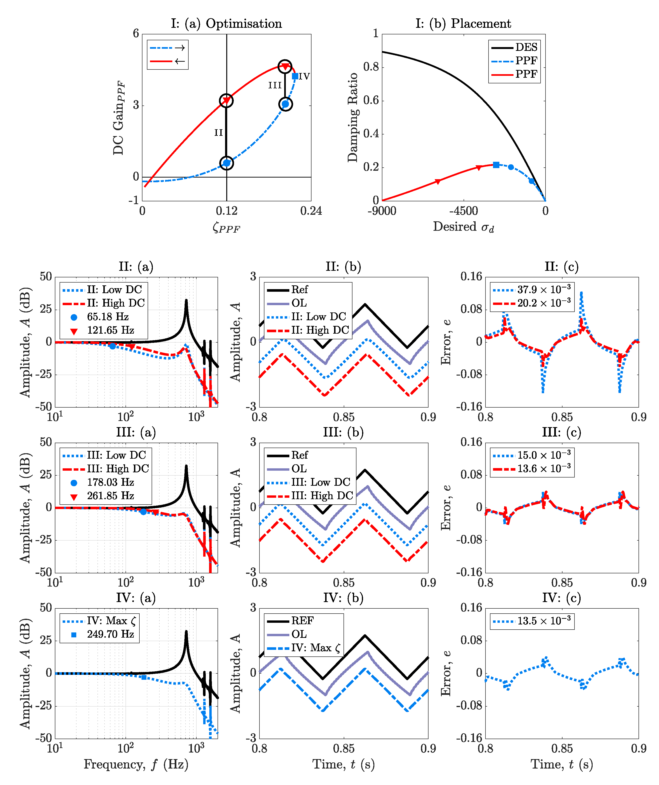
Figure 3a, each point on the optimisation curve represents an optimal PPF controller for the specified
. The optimisation curve has two key sections that make up the whole closed–loop curve, namely the blue dashed and red solid curves, respectively. As the poles move from
, this represents the blue dashed curve in which the PPF controller reaches its maximum possible damping of
. This curve also corresponds to the low DC gain that is possible for a given damping ratio. At this key value, no more extra damping of the closed–loop system is possible, and it is rendered as the final ‘optimal point’ in terms of just damping. As the poles move from
, this represents the red solid curve in which the PPF controller travels back across the same achieved closed–loop damping values but notably possesses higher DC gain for the same damping than the blue dashed curve. The difference between the upper and lower curves in terms of their DC gains matters greatly for tracking control but not for pure damping.
Figure 3(Ib) shows the difference between the obtained closed–loop damping, which is colour coded and noted in
Figure 3(Ia), and the desired closed–loop damping is in solid black. Due to the PPF optimisation problem being that of an over defined one in terms of the system of equations, this does not allow for complete pole–placement. This causes the desired damping and actual obtained closed–loop damping to differ hugely, as confirmed in
Figure 3(Ib). If damping is the only application required for PPF control, then selecting the maximum damping on the closed–loop optimisation curve will yield the best results; however, for tracking control, more needs to be considered. Simulation sets II and III show in detail the differences that can be found in tracking performance based on the DC gain of the PPF controller.
In simulation sets II through IV, an optimal tracker is fitted to each PPF controller using Equations (
17)–(
25). In
Figure 3(IIa–c), two PPF controllers are derived at the same damping ratio of
with different DC gains of
dB and
dB, respectively. In
Figure 3(IIa), the low and high DC gain
dB bandwidths are
and
, respectively.
Figure 3(IIb,c) show the difference in tracking the
triangle wave and confirms that the higher DC gain PPF controller has a lower closed–loop error when compared with the lower DC gain PPF controller. The RMS errors of the low and high DC controllers are that of
and
, respectively. A similar result is also found in
Figure 3(IIIa–c)
dB, where the bandwidths are
and
, respectively. Further notice that increasing the RMS errors of the low and high DC controllers are that of
and
, respectively, the difference in which is the low and high DC gain. This is a key result with respect to tracking applications that also require damping. The higher the frequency is for the
dB point, the smaller the closed–loop tracking error is. As such, in a tracking application involving PPF, the higher DC gain at a specific damping ratio should always be selected. Overall, due to PPF not providing complete pole–placement, this control scheme is not recommended for both damping or damping and tracking applications. The next section considers PVPF control as a superior solution to PPF’s shortcomings.
5. PVPF Optimisation and Analysis
To begin with optimising PVPF control, the matrix system of Equation (
12) needs to be reduced accordingly. Setting
to zero in this system will yield the PVPF controller and, hence, the following derived system of equations:
Unlike in the PPF case, it is highly important to note a key feature of matrix equation (
27). This system of equations is determined and features the same amount of equations and unknowns. Mathematically speaking, there are four equations and four unknowns giving rise to singular solutions for this system for a specific damping ratio, unlike in the PPF case with the co-existence of solutions. The result of having a determined system of equations in PVPF control is that pole–zero–placement is practically possible, unlike in the case of PPF control. Consider the following group of simulations detailing the closed–loop behaviour of PVPF control.
For the optimisation procedure of PVPF control, the system of Equation in (
27) is used with the dominant resonant mode system values of
,
,
and
, respectively. The poles of closed–loop system are varied such that
. In
Figure 4(Ia), the graph of the DC gain versus closed–loop damping is shown. Due to pole–placement being possible with PVPF control, unlike in PPF control, singular unique DC gains are found for each damping ratio considered. This is a direct result of PVPF control providing a determined system of equations.
Figure 4(Ib) confirms pole–placement as the desired curve in solid black aligns with the closed–loop blue dashed PVPF line.
In simulation sets II through IV, an optimal tracker is fitted to each PVPF controller using Equations (
17)–(
25).
Figure 4(IIa–c) shows the behaviour of the PVPF controller at the maximum DC gain point located at a damping ratio of
. The
dB bandwidth is located at
and results in an rms error of
when the reference and closed–loop output are phase compensated. When looking at
Figure 4(IIa–c), the
dB bandwidth shifts down to
, but the rms error decreases overall to
due to the extra damping imparted, namely
. This shows that there is a substantial difference in rms error and, hence, tracking performance between II and III, which is notable.
Figure 4(IVa–c) show that by going into the negative DC gain, the
bandwidth shifts to
. This results in the rms error reducing to
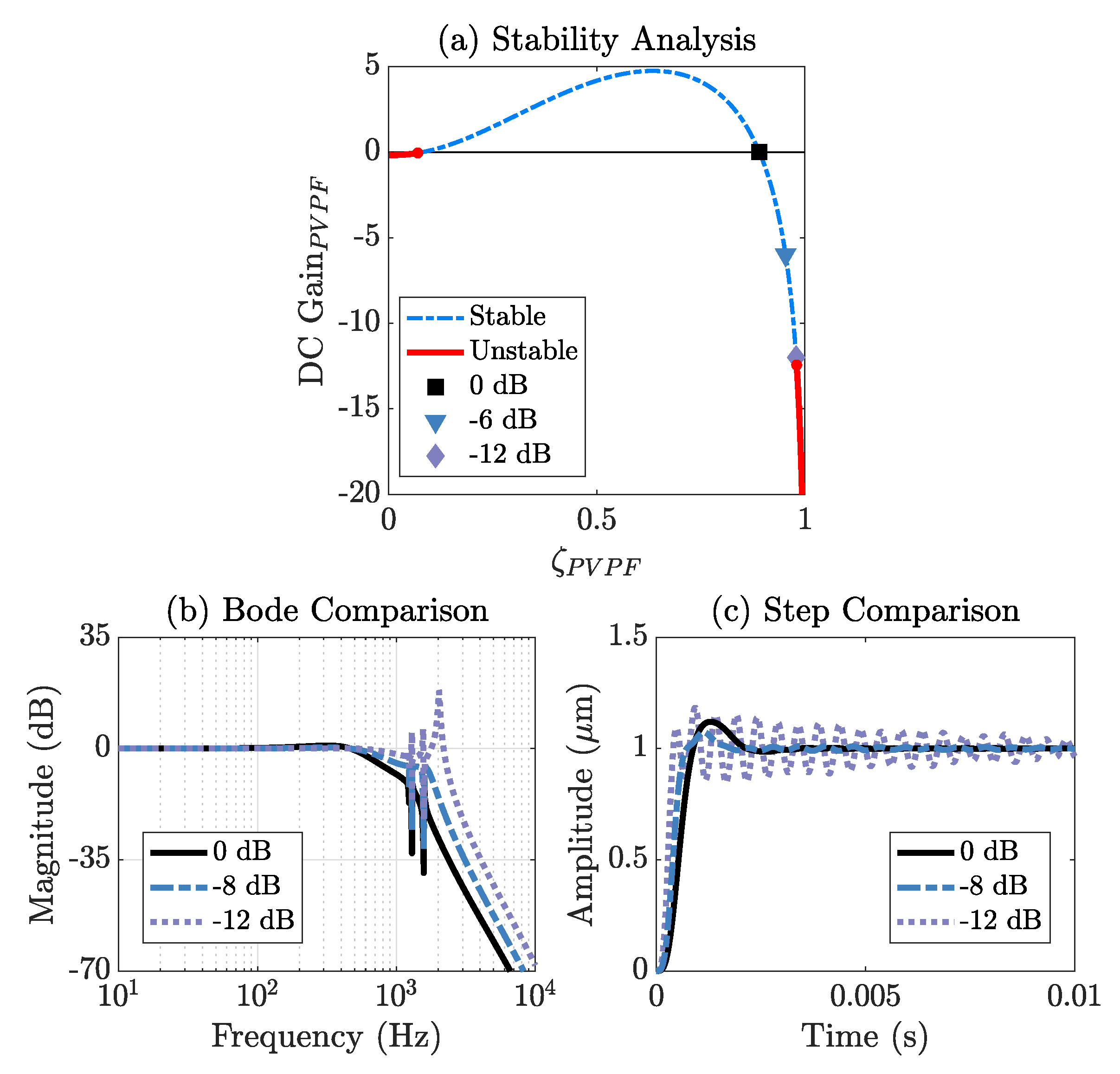
. To further understand PVPF’s limits, examining the closed–loop response and limits of stability as the damping increases are necessary. The following figure covers the aforementioned concerns:
Figure 5b,c highlights the downsides of pushing the damping up to the natural limit before instability. By going beyond and into negative DC gain PVPF controllers, the damping of the primary resonant mode becomes better as expected, but this comes at the downside of raising the closed–loop system response near other system modes. As a result, this can negatively affect impulse and step responses as well as signal tracking for frequencies in and around these system modes. Three controllers, namely,
,
and
, are represented by solid black (square mark), dashed-dotted blue (inverted triangle) and dashed lavender (diamond), respectively. The PVPF controller
, which is near the unstable point calculated, highlights this feature in which its amplitude response raises well above the
dB point for frequencies beyond the main resonance. This has the negative consequence of affecting the settling time greatly in the case of step and impulse responses as these signal types invoke infinitely many frequencies in their inception, thereby exciting these higher frequency dynamics that have been put above the crucial
dB point.
also demonstrates a key piece of behaviour, namely that a new resonance is introduced into the system at
. By forcing the system too much, the closed–loop dynamics change significantly. The controller
does not suffer from these effects nearly as much as in the
case because it does not raise the higher frequency dynamics to be above that of the
dB point. The settling time between the two controllers
and
is comparable; however, there is more oscillatory behaviour in the step response between these two found in that of
; this is due to the fact that
raises the higher frequency components above the primary damped resonance, albeit these frequencies are still under the critical
dB point.
6. PAVPF Part I: Optimisation and Analysis
In this section, PAVPF control is simulated and discussed in detail. Comparisons with PVPF are drawn directly, and a complete understanding is reached with respect to PAVPF control. To begin with optimising PAVPF control, the original derived system of Equation (
12) is used directly. Unlike in the PVPF case, it is highly important to note a key feature of matrix Equation (
28). This system of equations is underdetermined and features fewer equations than unknowns. Unlike in the case of PPF, which is also underdetermined, complete pole–placement is achievable with PAPVF control due to the system of Equation (
12) being an augmented PVPF problem. To this end, due to the time and bode responses found in PVPF being effectively the same as the ones that would be found with PAVPF, only comparisons with the DC gain versus damping graphs, as seen in
Figure 4(Ia), are required. Consider the following simulations:
In
Figure 6, PAVPF’s DC gain versus closed–loop damping is considered as per
and its subsets defined in the figure caption.
Figure 6c–f provide the individual responses found for the comparisons between them in
Figure 6a,b. The ranges for
are chosen arbitrarily in order to demonstrate the nature of overdetermined PAVPF when compared with PVPF and to further demonstrate how changing the range of possible
can affect optimal damping solutions.
Figure 6c is the same PVPF curve as defined before and is used for baseline comparisons.
Figure 6d–f show PAVPF with the full range of defined
, a restricted range of
for positive reals and lastly, another restricted range for negative reals starting at
to the same upper bound defined in
.
Figure 6d shows that with a generous range of values for
, a zig-zag pattern between DC gain and closed–loop damping is observed throughout the whole response as the poles are pushed further into the left-hand-plane subject to
. This zig-zag pattern’s maximum and minimum DC gain decreases as the damping increases all the way up to a maximum damping of
in which, after this point, the DC gain goes negative in a similar fashion with PVPF when the poles are pushed further.
Figure 6e shows the effects of limiting the
to only positive reals. This figure traces out a curve identical to that of PVPF up until the critical damping was found to be
. When compared with
Figure 6d, this directly implies that negative
values are found to be optimal before this key damping value, and since
Figure 6e has no negative
values, the optimisation curve is forced to follow that of the PVPF curve up to the aforementioned damping.
Figure 6f confirms this as well since it allows for the use of small negative
values down to
and upwards, and it follows a trajectory similar to that of
Figure 6d up until a damping value of
in which it branches off and follows a path defined by the last optimal
found here and rejoins the other curves at the critical damping of
. The common theme between all PAVPF curves is at they all rejoin at the closed–loop damping of
for an optimal
, and this is shown in detail in
Figure 6a, which compares
Figure 6d–f directly.
The most important conclusion that can be drawn from the PAVPF optimisation curves is namely that of
Figure 6b, which compares the base PVPF with the positive real restricted PAVPF responses directly. This comparison highlights that by using PAVPF, extra damping can be achieved compared with PAVPF without going into large negative DC gain values (viz
). More specifically, PVPF produces a maximum damping of
versus the maximum damping PAVPF produces of
without dropping into large negative DC gains. This gain in damping for the extra complexity of PAVPF on a second–order model is not worth it, given that the closed–loop time histories will be virtually identical and also the drop in the closed–loop tracking error would also not be greatly improved either. As a result, to better utilise PAVPF and understand its effects, it must be applied to a third–order system instead of a second–order one in order to avoid the underdetermined nature of system (
12). The following section deals with the optimisation of PAVPF on a third–order system to address these concerns.
7. Pavpf Part II: Adapting the Problem
Since the PAVPF controller is underdetermined, as discussed earlier, a third–order model is required in order to produce proper pole–placement and meet the condition of a properly determined system. Consider the following third–order model:
where
is the cut–off frequency of a first–order filter. This first–order filter can represent sensor dynamics or amplifier dynamics that do not scale or affect the DC gain of the plant in question and are effectively part of the whole system in question. As a result, the following closed–loop system is defined as follows:
This closed–loop system has the following DC gain function:
Notice that this function, unlike in Equation (
15), is not dependent on
due to the third–order system being used for pole–placement purposes. The denominator coefficients for Equation (
30) can be seen in
Table 6 as follows.
To deal with the proper pole–placement of this system with PAVPF control, a fifth–order polynomial is required. To this end, the same poles discussed earlier are re-used, except an additional pole is introduced corresponding to the effective pole that the amplifier circuit applies to the closed–loop system:
Then the desired characteristic polynomial
that has the roots given by Equation (
32) is defined as:
where the desired coefficients can be seen in
Table 7.
In order to perform pole–placement between the desired polynomial (
33) and the coefficients defined in
Table 7, they are set equal to one another as follows;
As before, this allows for a determined system of matrix equations to be generated as follows:
where
,
and
, respectively.
Q,
and
are as follows;
and
In the following comparison, the amplifier sensor’s cut–off frequency
is used as the additional pole introduced in this third–order system. Consider the following comparison in
Figure 7.
By properly conditioning PAVPF control on a third–order system as defined previously, this produces a virtually identical optimisation curve when compared with PVPF control on the second–order system as seen in
Figure 7. PAVPF implemented on the second–order system, which is overdetermined, allows for extra damping while keeping the DC gain close to zero. As a result, even though time histories would not show much difference between
and
on PAVPF determined and PAVPF overdetermined, overdetermined PAVPF still provides more possible damping while keeping the DC gain close to zero. This implies that overdetermined PAVPF is more optimal for damping versus determined PAVPF, which also includes damping with tracking as well.
8. Concluding Remarks
This paper addresses a long–standing knowledge gap with respect to a second–order damping system and how far to push the closed–loop poles of the system in question, as well as addressing the concept of determined, underdetermined and overdetermined optimisation problems with respect to pole–placement. Since PAVPF control encodes PVPF and PPF control, respectively, the optimisation process is designed around PAVPF first. A general blueprint for PPF, PVPF and PAVPF damping optimisation is obtained by converting the pole–placement strategy into its matrix form on a second–order system. This matrix form begins in an underdetermined form due to PAVPF requiring a third–order system for proper pole–placement. Subsequent to this, PVPF and PPF pole–placement methodologies are derived from this blueprint by omitting the acceleration term as well as the acceleration and velocity terms, respectively. In the final part of the paper, a fully determined form for PAVPF is developed in a similar manner to PVPF and then analysed and compared to fully determined PAVPF and overdetermined PAVPF.
Overall, the most pivotal result is found within the comparisons between PAVPF and PVPF control when PAVPF is made to be overdetermined and fully determined. Fully determined PAVPF is virtually identical to fully determined PVPF in terms of the optimal DC gain versus the damping curve produced, and only the undetermined PAVPF optimisation procedure can produce additional damping over its regular fully determined counterpart.


