
Impact of Reference Data Sampling Density for Estimating Plot-Level Average Shrub Heights Using Terrestrial Laser Scanning Data
 , ,
, ,  and
and
Abstract
:1. Introduction
2. Background
3. Methods
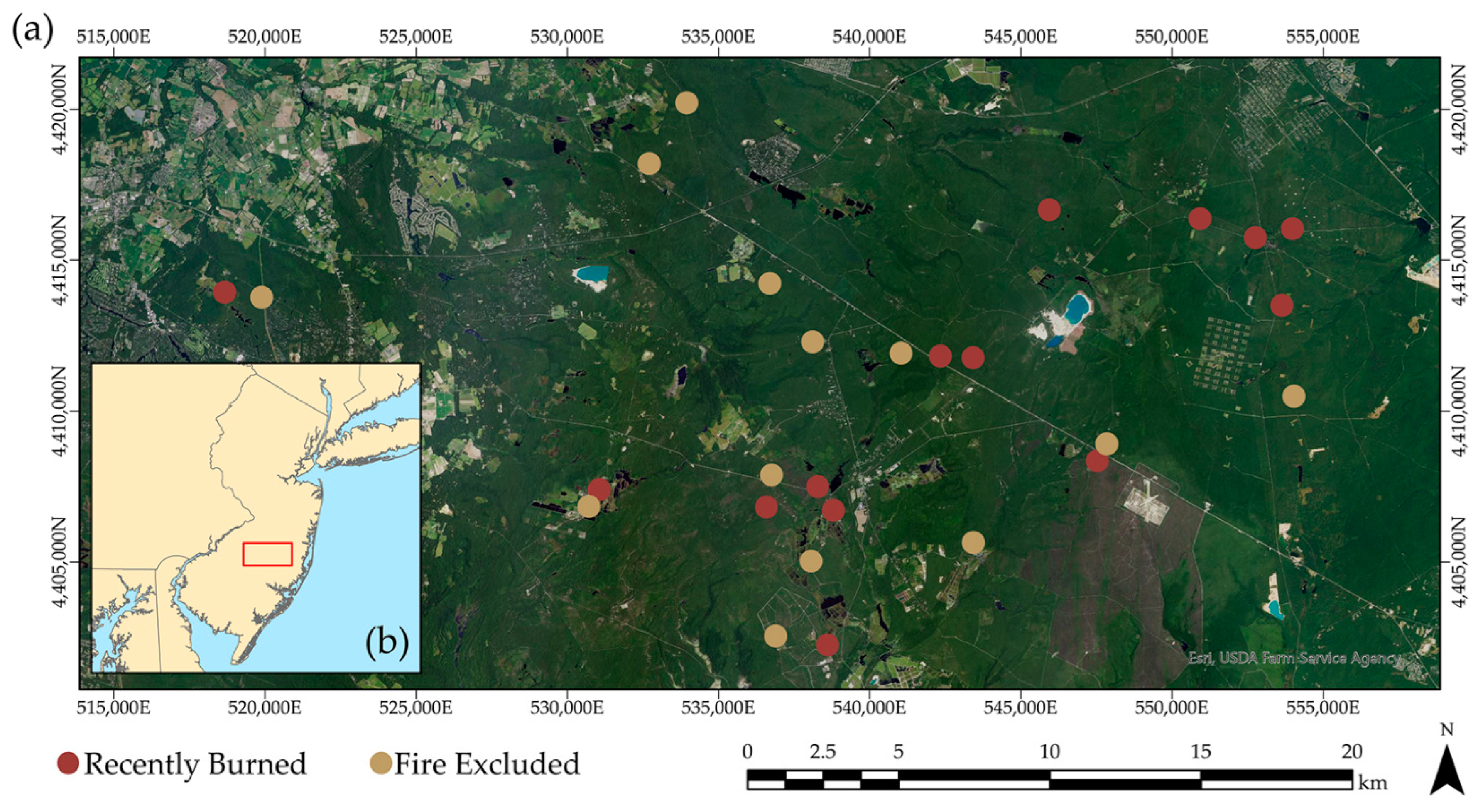
3.1. Study Area
3.2. TLS and Ground Data
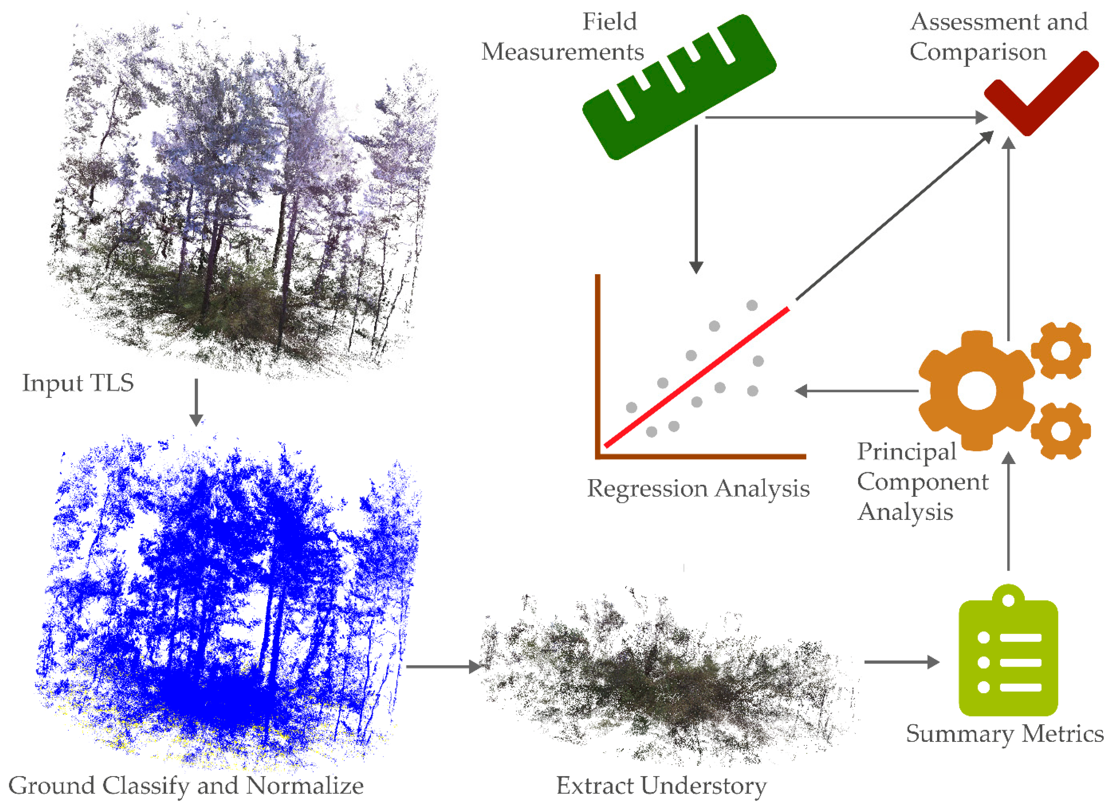
3.3. Data Preparation
3.4. Regression Modeling
3.5. Assessment and Comparison
4. Results and Discussion
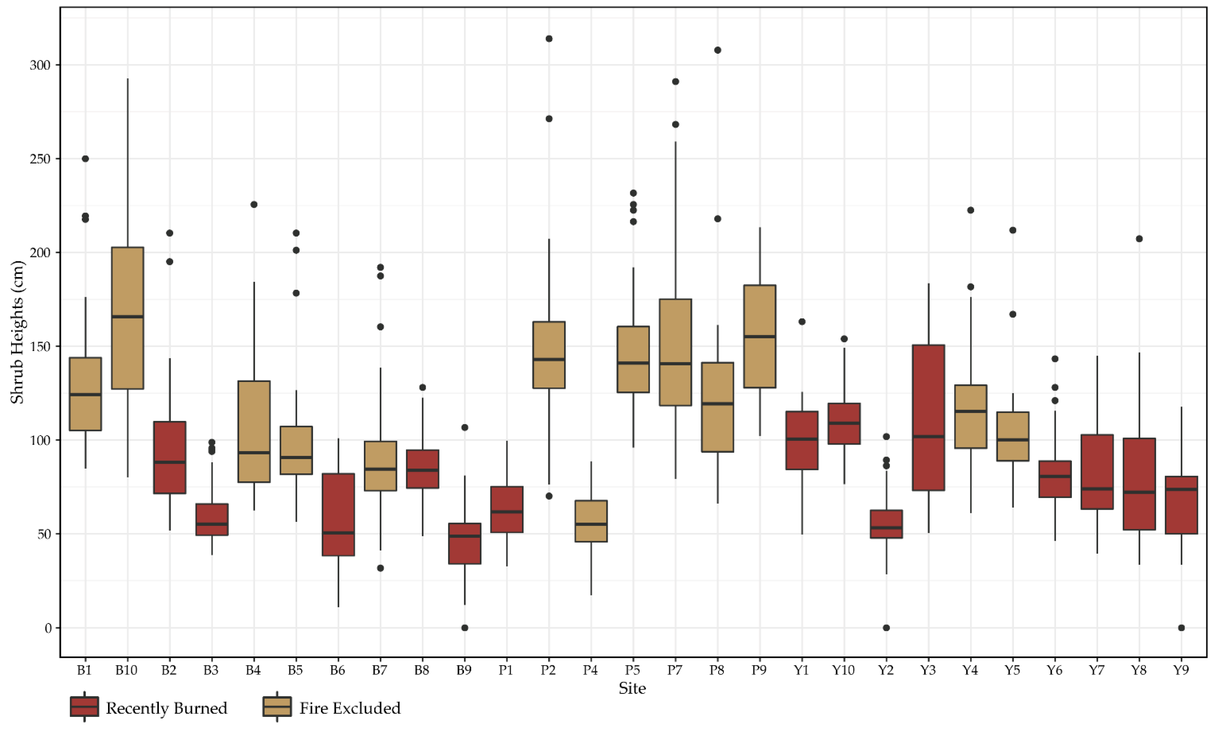
4.1. Distribution of Shrub Heights within Plots
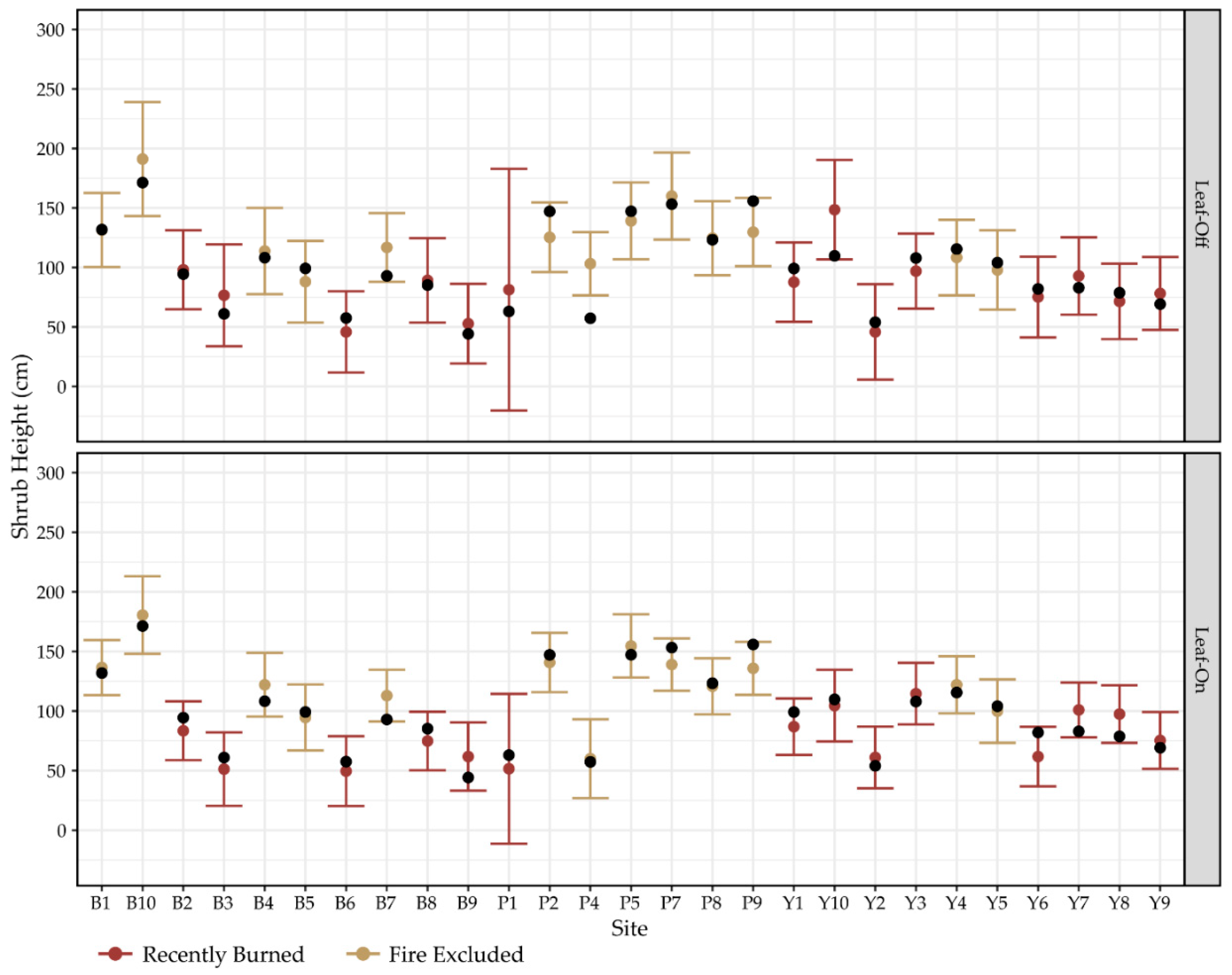
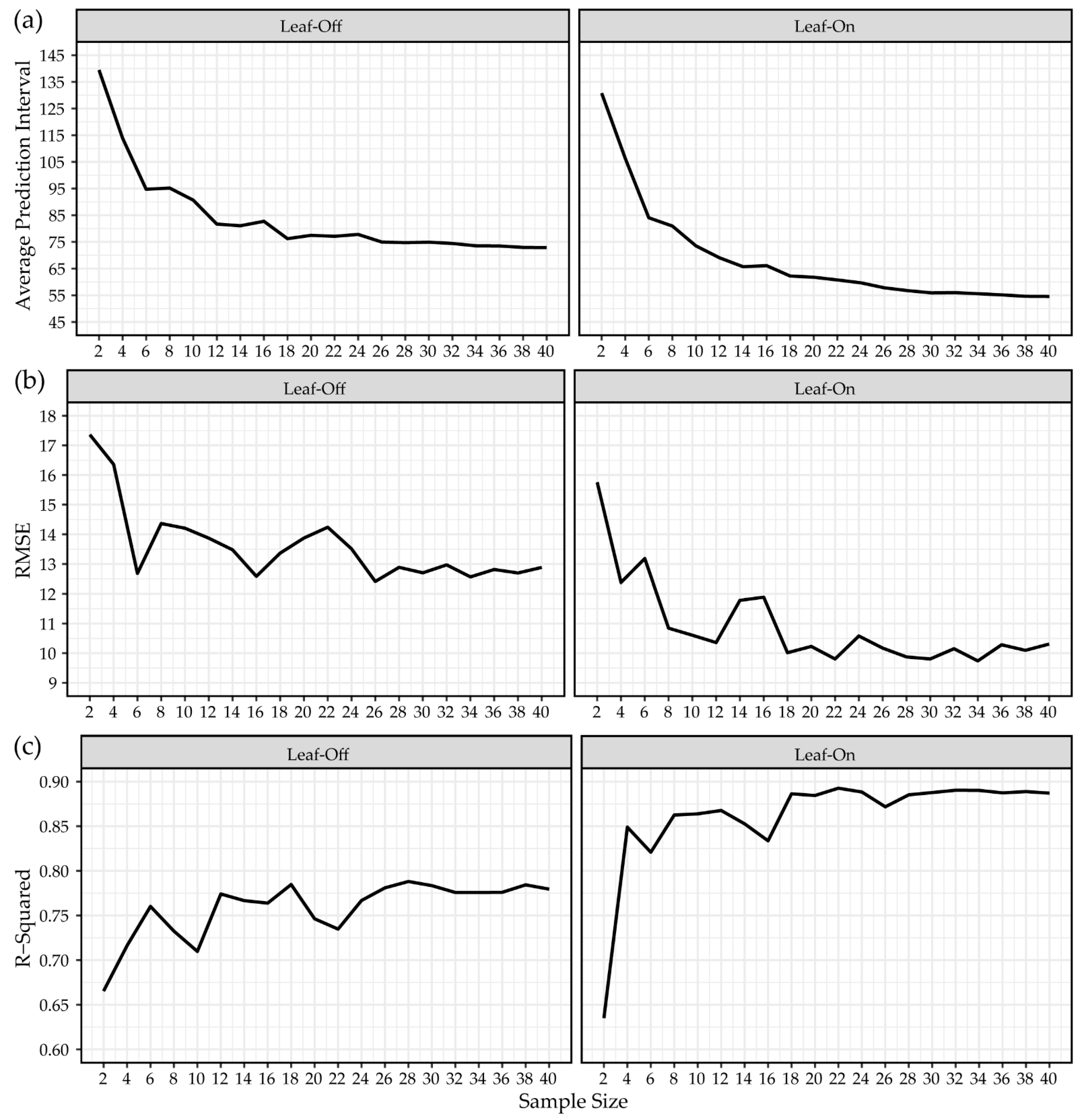
4.2. Impact of Number of Shrub Height Measurements and Phenology on Model Performance
5. Conclusions
Author Contributions
Funding
Data Availability Statement
Acknowledgments
Conflicts of Interest
References
- Finney, M.A.; McAllister, S.S.; Forthofer, J.M.; Grumstrup, T.P. Wildland Fire Behaviour: Dynamics, Principles and Processes; CSIRO Publishing: Clayton, Australia, 2021. [Google Scholar]
- Rego, F.C.; Morgan, P.; Fernandes, P.; Hoffman, C. Fire Science: From Chemistry to Landscape Management; Springer Nature: Berlin, Germany, 2021. [Google Scholar]
- Harvey, B.J. Human-caused climate change is now a key driver of forest fire activity in the western United States. Proc. Natl. Acad. Sci. USA 2016, 113, 11649–11650. [Google Scholar] [CrossRef] [Green Version]
- Cary, G.J.; Flannigan, M.D.; Keane, R.E.; Bradstock, R.A.; Davies, I.D.; Lenihan, J.M.; Li, C.; Logan, K.A.; Parsons, R.A. Relative importance of fuel management, ignition management and weather for area burned: Evidence from five landscape–fire–succession models. Int. J. Wildland Fire 2009, 18, 147–156. [Google Scholar] [CrossRef] [Green Version]
- Knapp, E.E.; Keeley, J.E.; Ballenger, E.A.; Brennan, T.J. Fuel reduction and coarse woody debris dynamics with early season and late season prescribed fire in a Sierra Nevada mixed conifer forest. For. Ecol. Manag. 2005, 208, 383–397. [Google Scholar] [CrossRef]
- McCaw, W.L. Managing forest fuels using prescribed fire—A perspective from southern Australia. For. Ecol. Manag. 2013, 294, 217–224. [Google Scholar] [CrossRef]
- Safford, H.D.; Schmidt, D.A.; Carlson, C.H. Effects of fuel treatments on fire severity in an area of wildland–urban interface, Angora Fire, Lake Tahoe Basin, California. For. Ecol. Manag. 2009, 258, 773–787. [Google Scholar] [CrossRef]
- Hoffman, C.M.; Sieg, C.H.; Linn, R.R.; Mell, W.; Parsons, R.A.; Ziegler, J.P.; Hiers, J.K. Advancing the Science of Wildland Fire Dynamics Using Process-Based Models. Fire 2018, 1, 32. [Google Scholar] [CrossRef] [Green Version]
- Parsons, R.A.; Mell, W.E.; McCauley, P. Linking 3D spatial models of fuels and fire: Effects of spatial heterogeneity on fire behavior. Ecol. Model. 2011, 222, 679–691. [Google Scholar] [CrossRef]
- Pimont, F.; Parsons, R.; Rigolot, E.; de Coligny, F.; Dupuy, J.-L.; Dreyfus, P.; Linn, R.R. Modeling fuels and fire effects in 3D: Model description and applications. Environ. Model. Softw. 2016, 80, 225–244. [Google Scholar] [CrossRef] [Green Version]
- Pimont, F.; Dupuy, J.-L.; Linn, R.R.; Parsons, R.; Martin-StPaul, N. Representativeness of wind measurements in fire experiments: Lessons learned from large-eddy simulations in a homogeneous forest. Agric. For. Meteorol. 2017, 232, 479–488. [Google Scholar] [CrossRef]
- Wu, Z.; He, H.S.; Fang, L.; Liang, Y.; Parsons, R.A. Wind speed and relative humidity influence spatial patterns of burn severity in boreal forests of northeastern China. Ann. For. Sci. 2018, 75, 66. [Google Scholar] [CrossRef] [Green Version]
- Nelson, R.M.J. A method for describing equilibrium moisture content of forest fuels. Can. J. For. Res. 1984, 14, 597–600. [Google Scholar] [CrossRef] [Green Version]
- Viegas, D.X.; Viegas, M.; Ferreira, A.D. Moisture Content of Fine Forest Fuels and Fire Occurrence in Central Portugal. Int. J. Wildland Fire 1992, 2, 69–86. [Google Scholar] [CrossRef]
- Stephens, S.L.; Battaglia, M.A.; Churchill, D.J.; Collins, B.M.; Coppoletta, M.; Hoffman, C.M.; Lydersen, J.M.; North, M.P.; Parsons, R.A.; Ritter, S.M.; et al. Forest Restoration and Fuels Reduction: Convergent or Divergent? BioScience 2021, 71, 85–101. [Google Scholar] [CrossRef]
- Parsons, R.; Jolly, W.M.; Hoffman, C.; Ottmar, R. The role of fuels in extreme fire behavior. In Synthesis of Knowledge of Extreme Fire Behavior; U.S. Department of Agriculture, Forest Service, Pacific Northwest Research Station: Portland, OR, USA, 2016; p. 55. Available online: https://www.fs.usda.gov/research/treesearch/50530 (accessed on 17 February 2023).
- Loudermilk, E.L.; O’Brien, J.J.; Mitchell, R.J.; Cropper, W.P.; Hiers, J.K.; Grunwald, S.; Grego, J.; Fernandez-Diaz, J.C. Linking complex forest fuel structure and fire behaviour at fine scales. Int. J. Wildland Fire 2012, 21, 882–893. [Google Scholar] [CrossRef]
- Hiers, J.K.; O’Brien, J.J.; Varner, J.M.; Butler, B.W.; Dickinson, M.; Furman, J.; Gallagher, M.; Godwin, D.; Goodrick, S.L.; Hood, S.M.; et al. Prescribed fire science: The case for a refined research agenda. Fire Ecol. 2020, 16, 11. [Google Scholar] [CrossRef] [Green Version]
- Mitchell, R.J.; Hiers, J.K.; O’Brien, J.J.; Jack, S.B.; Engstrom, R.T. Silviculture that sustains: The nexus between silviculture, frequent prescribed fire, and conservation of biodiversity in longleaf pine forests of the southeastern United States. Can. J. For. Res. 2006, 36, 2724–2736. [Google Scholar] [CrossRef] [Green Version]
- Rothermel, R.C. A Mathematical Model for Predicting Fire Spread in Wildland Fuels; Intermountain Forest & Range Experiment Station, Forest Service, US Department of Agriculture: Ogden, UT, USA, 1972; Volume 115. Available online: https://www.fs.usda.gov/research/treesearch/32533 (accessed on 17 February 2023).
- Parsons, R.A.; Linn, R.R.; Pimont, F.; Hoffman, C.; Sauer, J.; Winterkamp, J.; Sieg, C.H.; Jolly, W.M. Numerical Investigation of Aggregated Fuel Spatial Pattern Impacts on Fire Behavior. Land 2017, 6, 43. [Google Scholar] [CrossRef]
- Gale, M.G.; Cary, G.J.; Van Dijk, A.I.J.M.; Yebra, M. Forest fire fuel through the lens of remote sensing: Review of approaches, challenges and future directions in the remote sensing of biotic determinants of fire behaviour. Remote Sens. Environ. 2021, 255, 112282. [Google Scholar] [CrossRef]
- Skowronski, N.S.; Gallagher, M.R. Fuels Characterization Techniques. In Encyclopedia of Wildfires and Wildland-Urban Interface (WUI) Fires; Manzello, S.L., Ed.; Springer International Publishing: Cham, Switzerland, 2018; pp. 1–10. ISBN 978-3-319-51727-8. [Google Scholar]
- Skowronski, N.S.; Gallagher, M.R.; Warner, T.A. Decomposing the Interactions between Fire Severity and Canopy Fuel Structure Using Multi-Temporal, Active, and Passive Remote Sensing Approaches. Fire 2020, 3, 7. [Google Scholar] [CrossRef] [Green Version]
- McCarley, T.R.; Hudak, A.T.; Sparks, A.M.; Vaillant, N.M.; Meddens, A.J.; Trader, L.; Mauro, F.; Kreitler, J.; Boschetti, L. Estimating wildfire fuel consumption with multitemporal airborne laser scanning data and demonstrating linkage with MODIS-derived fire radiative energy. Remote Sens. Environ. 2020, 251, 112114. [Google Scholar] [CrossRef]
- Ross, C.W.; Loudermilk, E.L.; Skowronski, N.; Pokswinski, S.; Hiers, J.K.; O’Brien, J. LiDAR Voxel-Size Optimization for Canopy Gap Estimation. Remote Sens. 2022, 14, 1054. [Google Scholar] [CrossRef]
- Gallagher, M.R.; Cope, Z.; Giron, D.R.; Skowronski, N.S.; Raynor, T.; Gerber, T.; Linn, R.R.; Hiers, J.K. Reconstruction of the Spring Hill Wildfire and Exploration of Alternate Management Scenarios Using QUIC. Fire 2021, 4, 72. [Google Scholar] [CrossRef]
- Fernández-Álvarez, M.; Armesto, J.; Picos, J. LiDAR-based wildfire prevention in WUI: The automatic detection, measurement and evaluation of forest fuels. Forests 2019, 10, 148. [Google Scholar] [CrossRef] [Green Version]
- Gallagher, M.R.; Skowronski, N.S.; Lathrop, R.G.; McWilliams, T.; Green, E.J. An improved approach for selecting and validating burn severity indices in forested landscapes. Can. J. Remote Sens. 2020, 46, 100–111. [Google Scholar] [CrossRef]
- Sandberg, D.V.; Ottmar, R.D.; Cushon, G.H. Characterizing fuels in the 21st Century. Int. J. Wildland Fire 2001, 10, 381–387. [Google Scholar] [CrossRef]
- Wallace, L.; Hillman, S.; Hally, B.; Taneja, R.; White, A.; McGlade, J. Terrestrial Laser Scanning: An Operational Tool for Fuel Hazard Mapping? Fire 2022, 5, 85. [Google Scholar] [CrossRef]
- Stovall, A.E.L.; Atkins, J.W. Assessing Low-Cost Terrestrial Laser Scanners for Deriving Forest Structure Parameters. Preprints 2021. [Google Scholar] [CrossRef]
- Pokswinski, S.; Gallagher, M.R.; Skowronski, N.S.; Loudermilk, E.L.; Hawley, C.; Wallace, D.; Everland, A.; Wallace, J.; Hiers, J.K. A simplified and affordable approach to forest monitoring using single terrestrial laser scans and transect sampling. MethodsX 2021, 8, 101484. [Google Scholar] [CrossRef]
- Brown, J.K. Bulk Densities of Nonuniform Surface Fuels and Their Application to Fire Modeling. For. Sci. 1981, 27, 667–683. [Google Scholar] [CrossRef]
- Hines, F.; Hines, F.; Tolhurst, K.G.; Wilson, A.A.; McCarthy, G.J. Overall Fuel Hazard Assessment Guide; Victorian Government, Department of Sustainability and Environment Melbourne: 2010. Available online: https://www.ffm.vic.gov.au/__data/assets/pdf_file/0005/21110/Report-82-overall-fuel-assess-guide-4th-ed.pdf (accessed on 17 February 2023).
- Brown, J.K. Handbook for Inventorying Downed Woody Material; US Department of Agriculture, Forest Service, Intermountain Forest and Range Experiment Station: Ogden, UT, USA, 1974; p. 16. [Google Scholar]
- Sikkink, P.G.; Keane, R.E.; Sikkink, P.G.; Keane, R.E. A comparison of five sampling techniques to estimate surface fuel loading in montane forests. Int. J. Wildland Fire 2008, 17, 363–379. [Google Scholar] [CrossRef]
- Keane, R.E.; Gray, K.; Keane, R.E.; Gray, K. Comparing three sampling techniques for estimating fine woody down dead biomass. Int. J. Wildland Fire 2013, 22, 1093–1107. [Google Scholar] [CrossRef] [Green Version]
- Westfall, J.A.; Woodall, C.W. Measurement repeatability of a large-scale inventory of forest fuels. For. Ecol. Manag. 2007, 253, 171–176. [Google Scholar] [CrossRef]
- Kessell, S.R.; Potter, M.W.; Bevins, C.D.; Bradshaw, L.; Jeske, B.W. Analysis and application of forest fuels data. Environ. Manag. 1978, 2, 347–363. [Google Scholar] [CrossRef]
- Prichard, S.J.; Sandberg, D.V.; Ottmar, R.D.; Eberhardt, E.; Andreu, A.; Eagle, P.; Swedin, K. Fuel Characteristic Classification System Version 3.0: Technical Documentation; Gen. Tech. Rep. PNW-GTR-887; US Department of Agriculture, Forest Service, Pacific Northwest Research Station: Portland, OR, USA, 2013; Volume 887, 79p.
- Arroyo, L.A.; Pascual, C.; Manzanera, J.A. Fire models and methods to map fuel types: The role of remote sensing. For. Ecol. Manag. 2008, 256, 1239–1252. [Google Scholar] [CrossRef] [Green Version]
- Mutlu, M.; Popescu, S.C.; Stripling, C.; Spencer, T. Mapping surface fuel models using lidar and multispectral data fusion for fire behavior. Remote Sens. Environ. 2008, 112, 274–285. [Google Scholar] [CrossRef]
- García, M.; Riaño, D.; Chuvieco, E.; Salas, J.; Danson, F.M. Multispectral and LiDAR data fusion for fuel type mapping using Support Vector Machine and decision rules. Remote Sens. Environ. 2011, 115, 1369–1379. [Google Scholar] [CrossRef]
- Erdody, T.L.; Moskal, L.M. Fusion of LiDAR and imagery for estimating forest canopy fuels. Remote Sens. Environ. 2010, 114, 725–737. [Google Scholar] [CrossRef]
- Skowronski, N.S.; Clark, K.L.; Duveneck, M.; Hom, J. Three-dimensional canopy fuel loading predicted using upward and downward sensing LiDAR systems. Remote Sens. Environ. 2011, 115, 703–714. [Google Scholar] [CrossRef]
- Peterson, B.; Nelson, K.J.; Seielstad, C.; Stoker, J.; Jolly, W.M.; Parsons, R. Automated integration of lidar into the LANDFIRE product suite. Remote Sens. Lett. 2015, 6, 247–256. [Google Scholar] [CrossRef]
- Lillesand, T.; Kiefer, R.W.; Chipman, J. Remote Sensing and Image Interpretation; John Wiley & Sons: Hoboken, NJ, USA, 2015. [Google Scholar]
- Skowronski, N.S.; Haag, S.; Trimble, J.; Clark, K.L.; Gallagher, M.R.; Lathrop, R.G.; Skowronski, N.S.; Haag, S.; Trimble, J.; Clark, K.L.; et al. Structure-level fuel load assessment in the wildland–urban interface: A fusion of airborne laser scanning and spectral remote-sensing methodologies. Int. J. Wildland Fire 2015, 25, 547–557. [Google Scholar] [CrossRef]
- Skowronski, N.; Clark, K.; Nelson, R.; Hom, J.; Patterson, M. Remotely sensed measurements of forest structure and fuel loads in the Pinelands of New Jersey. Remote Sens. Environ. 2007, 108, 123–129. [Google Scholar] [CrossRef]
- Alonso-Rego, C.; Arellano-Pérez, S.; Guerra-Hernández, J.; Molina-Valero, J.A.; Martínez-Calvo, A.; Pérez-Cruzado, C.; Castedo-Dorado, F.; González-Ferreiro, E.; Álvarez-González, J.G.; Ruiz-González, A.D. Estimating Stand and Fire-Related Surface and Canopy Fuel Variables in Pine Stands Using Low-Density Airborne and Single-Scan Terrestrial Laser Scanning Data. Remote Sens. 2021, 13, 5170. [Google Scholar] [CrossRef]
- Loudermilk, E.L.; Hiers, J.K.; O’Brien, J.J.; Mitchell, R.J.; Singhania, A.; Fernandez, J.C.; Cropper, W.P.; Slatton, K.C.; Loudermilk, E.L.; Hiers, J.K.; et al. Ground-based LIDAR: A novel approach to quantify fine-scale fuelbed characteristics. Int. J. Wildland Fire 2009, 18, 676–685. [Google Scholar] [CrossRef] [Green Version]
- Rowell, E.; Loudermilk, E.L.; Hawley, C.; Pokswinski, S.; Seielstad, C.; Queen, L.; O’Brien, J.J.; Hudak, A.T.; Goodrick, S.; Hiers, J.K. Coupling terrestrial laser scanning with 3D fuel biomass sampling for advancing wildland fuels characterization. For. Ecol. Manag. 2020, 462, 117945. [Google Scholar] [CrossRef]
- Rowell, E.; Loudermilk, E.L.; Seielstad, C.; O’Brien, J.J. Using Simulated 3D Surface Fuelbeds and Terrestrial Laser Scan Data to Develop Inputs to Fire Behavior Models. Can. J. Remote Sens. 2016, 42, 443–459. [Google Scholar] [CrossRef]
- Alonso-Rego, C.; Arellano-Pérez, S.; Cabo, C.; Ordoñez, C.; Álvarez-González, J.G.; Díaz-Varela, R.A.; Ruiz-González, A.D. Estimating Fuel Loads and Structural Characteristics of Shrub Communities by Using Terrestrial Laser Scanning. Remote Sens. 2020, 12, 3704. [Google Scholar] [CrossRef]
- García, M.; Danson, F.M.; Riaño, D.; Chuvieco, E.; Ramirez, F.A.; Bandugula, V. Terrestrial laser scanning to estimate plot-level forest canopy fuel properties. Int. J. Appl. Earth Obs. Geoinf. 2011, 13, 636–645. [Google Scholar] [CrossRef]
- Rowell, E.M.; Seielstad, C.A.; Ottmar, R.D.; Rowell, E.M.; Seielstad, C.A.; Ottmar, R.D. Development and validation of fuel height models for terrestrial lidar—RxCADRE 2012. Int. J. Wildland Fire 2015, 25, 38–47. [Google Scholar] [CrossRef]
- Hudak, A.T.; Kato, A.; Bright, B.C.; Loudermilk, E.L.; Hawley, C.; Restaino, J.C.; Ottmar, R.D.; Prata, G.A.; Cabo, C.; Prichard, S.J.; et al. Towards Spatially Explicit Quantification of Pre- and Postfire Fuels and Fuel Consumption from Traditional and Point Cloud Measurements. For. Sci. 2020, 66, 428–442. [Google Scholar] [CrossRef]
- Gallagher, M.R.; Maxwell, A.E.; Guillén, L.A.; Everland, A.; Loudermilk, E.L.; Skowronski, N.S. Estimation of Plot-Level Burn Severity Using Terrestrial Laser Scanning. Remote Sens. 2021, 13, 4168. [Google Scholar] [CrossRef]
- Key, C.H.; Benson, N.C. Landscape assessment (LA). In FIREMON: Fire Effects Monitoring and Inventory System; Lutes, D.C., Keane, R.E., Caratti, J.F., Key, C.H., Benson, N.C., Sutherland, S., Gangi, L.J., Eds.; Gen. Tech. Rep. RMRS-GTR-164-CD; US Department of Agriculture, Forest Service, Rocky Mountain Research Station: Fort Collins, CO, USA, 2006; Volume 164, p. LA-1-55. [Google Scholar]
- Fassnacht, F.; Hartig, F.; Latifi, H.; Berger, C.; Hernández, J.; Corvalán, P.; Koch, B. Importance of sample size, data type and prediction method for remote sensing-based estimations of aboveground forest biomass. Remote Sens. Environ. 2014, 154, 102–114. [Google Scholar] [CrossRef]
- McRoberts, R.E.; Tomppo, E.O. Remote sensing support for national forest inventories. Remote Sens. Environ. 2007, 110, 412–419. [Google Scholar] [CrossRef]
- Plourde, L.; Congalton, R.G. Sampling method and sample placement: How do they affect the accuracy of remotely sensed maps. Photogramm. Eng. Remote Sens. 2003, 69, 289–297. [Google Scholar] [CrossRef]
- Foody, G.M. Assessing the accuracy of land cover change with imperfect ground reference data. Remote Sens. Environ. 2010, 114, 2271–2285. [Google Scholar] [CrossRef] [Green Version]
- Congalton, R.G. Accuracy assessment and validation of remotely sensed and other spatial information. Int. J. Wildland Fire 2001, 10, 321–328. [Google Scholar] [CrossRef] [Green Version]
- Olsoy, P.J.; Glenn, N.F.; Clark, P.E. Estimating Sagebrush Biomass Using Terrestrial Laser Scanning. Rangel. Ecol. Manag. 2014, 67, 224–228. [Google Scholar] [CrossRef]
- Calders, K.; Newnham, G.; Burt, A.; Murphy, S.; Raumonen, P.; Herold, M.; Culvenor, D.; Avitabile, V.; Disney, M.; Armston, J.; et al. Nondestructive estimates of above-ground biomass using terrestrial laser scanning. Methods Ecol. Evol. 2015, 6, 198–208. [Google Scholar] [CrossRef]
- Cooper, S.D.; Roy, D.P.; Schaaf, C.B.; Paynter, I. Examination of the Potential of Terrestrial Laser Scanning and Structure-from-Motion Photogrammetry for Rapid Nondestructive Field Measurement of Grass Biomass. Remote Sens. 2017, 9, 531. [Google Scholar] [CrossRef] [Green Version]
- Hillman, S.; Wallace, L.; Reinke, K.; Hally, B.; Jones, S.; Saldias, D.S. A Method for Validating the Structural Completeness of Understory Vegetation Models Captured with 3D Remote Sensing. Remote Sens. 2019, 11, 2118. [Google Scholar] [CrossRef] [Green Version]
- Hillman, S.; Wallace, L.; Lucieer, A.; Reinke, K.; Turner, D.; Jones, S. A comparison of terrestrial and UAS sensors for measuring fuel hazard in a dry sclerophyll forest. Int. J. Appl. Earth Obs. Geoinf. 2021, 95, 102261. [Google Scholar] [CrossRef]
- Rodríguez-Lozano, B.; Rodríguez-Caballero, E.; Maggioli, L.; Cantón, Y. Non-Destructive Biomass Estimation in Mediterranean Alpha Steppes: Improving Traditional Methods for Measuring Dry and Green Fractions by Combining Proximal Remote Sensing Tools. Remote Sens. 2021, 13, 2970. [Google Scholar] [CrossRef]
- Warner, T.A.; Skowronski, N.S.; La Puma, I. The influence of prescribed burning and wildfire on lidar-estimated forest structure of the New Jersey Pinelands National Reserve. Int. J. Wildland Fire 2020, 29, 1100–1108. [Google Scholar] [CrossRef]
- Forman, R.T.; Boerner, R.E. Fire frequency and the pine barrens of New Jersey. Bull. Torrey Bot. Club 1981, 108, 34–50. [Google Scholar] [CrossRef]
- Gallagher, M.R. Monitoring Fire Effects in the New Jersey Pine Barrens with Burn Severity Indices; Rutgers: New Brunswick, NJ, USA, 2017. [Google Scholar]
- R Core Team. R: A Language and Environment for Statistical Computing; R Foundation for Statistical Computing: Vienna, Austria, 2020. [Google Scholar]
- Roussel, J.-R.; Auty, D.; Coops, N.C.; Tompalski, P.; Goodbody, T.R.; Meador, A.S.; Bourdon, J.-F.; De Boissieu, F.; Achim, A. lidR: An R package for analysis of Airborne Laser Scanning (ALS) data. Remote Sens. Environ. 2020, 251, 112061. [Google Scholar] [CrossRef]
- de Conto, T.; Olofsson, K.; Görgens, E.B.; Rodriguez, L.C.E.; Almeida, G. Performance of stem denoising and stem modelling algorithms on single tree point clouds from terrestrial laser scanning. Comput. Electron. Agric. 2017, 143, 165–176. [Google Scholar] [CrossRef]
- Roussel, J.; Qi, J. RCSF: Airborne LiDAR Filtering Method Based on Cloth Simulation. R Package Version 2018, 1, 1. [Google Scholar]
- Evans, J.S. Spatialeco. R Package Version 1.3-6. 2021. Available online: https://github.com/jeffreyevans/spatialEco (accessed on 17 February 2023).
- Kuhn, M.; Johnson, K. Applied Predictive Modeling; Springer: Berlin/Heidelberg, Germany, 2013; Volume 26. [Google Scholar]
- Abdi, H.; Williams, L.J. Principal component analysis. Wiley Interdiscip. Rev. Comput. Stat. 2010, 2, 433–459. [Google Scholar] [CrossRef]
- Stine, R.A. Bootstrap prediction intervals for regression. J. Am. Stat. Assoc. 1985, 80, 1026–1031. [Google Scholar] [CrossRef]
- White, J.C.; Coops, N.C.; Wulder, M.A.; Vastaranta, M.; Hilker, T.; Tompalski, P. Remote sensing technologies for enhancing forest inventories: A review. Can. J. Remote Sens. 2016, 42, 619–641. [Google Scholar] [CrossRef] [Green Version]
- Bienert, A.; Georgi, L.; Kunz, M.; Maas, H.-G.; Von Oheimb, G. Comparison and combination of mobile and terrestrial laser scanning for natural forest inventories. Forests 2018, 9, 395. [Google Scholar] [CrossRef] [Green Version]
- Kaasalainen, S.; Krooks, A.; Liski, J.; Raumonen, P.; Kaartinen, H.; Kaasalainen, M.; Puttonen, E.; Anttila, K.; Mäkipää, R. Change detection of tree biomass with terrestrial laser scanning and quantitative structure modelling. Remote Sens. 2014, 6, 3906–3922. [Google Scholar] [CrossRef] [Green Version]
- Torresan, C.; Chiavetta, U.; Hackenberg, J. Applying quantitative structure models to plot-based terrestrial laser data to assess dendrometric parameters in dense mixed forests. For. Syst. 2018, 27, 1–15. [Google Scholar] [CrossRef] [Green Version]
- Zhu, Y.; Li, D.; Fan, J.; Zhang, H.; Eichhorn, M.; Wang, X.; Yun, T. A reinterpretation of the gap fraction of tree crowns from the perspectives of computer graphics and porous media theory. Front. Plant Sci. 2023, 14, 115. [Google Scholar] [CrossRef] [PubMed]


| Study | TLS Data | Ground Data | Parameters | Landscape |
|---|---|---|---|---|
| Loudermilk et al. (2009) [52] | Multiple scans; ILRIS | Point-intercept; fuel bed and litter depth; presence/absence of fuel; vegetation type (non-destructive) | Leaf biomass; leaf area; point-intercept volume | Longleaf pine (Georgia, USA) |
| Garcia et al. (2011) [56] | Multiple scans from the same position but rotated; Riegl LMS-Z390i | DBH; crown diameter, height, and base height; planar transects (non-destructive) | Canopy height, cover, and base height; fuel strata gap | Scots pine, larch, and mixed oak/birch (Cheshire, UK) |
| Loudermilk et al. (2012) [17] | Multiple scans; ILRIS | Point-intercept; forward-looking infrared (FLIR) thermal imaging | Maximum fire temperature and 90th quantile fire temperature; residence time at 300 °C and 500 °C | Longleaf pine (Georgia, USA) |
| Olsoy et al. (2014) [66] | Multiple scans; Riegl VZ-1000 | Point-intercept (non-destructive); harvesting of sagebrush (destructive) | Sagebrush biomass | Sagebrush (Idaho, USA) |
| Calders et al. (2015) [67] | Pre- and post-harvest multiple scans; Riegl VZ-400 | Forest inventory (destructive); tree DBH and height; stem maps; dry weight; AGB | Tree DBH and height; AGB | Eucalypt open forest (Victoria, AU) |
| Rowell et al. (2015) [54] | Multiple scans; Optech ILRIS 36D-HD | Clip plots (destructive); max and mean heights for grass, forbs, shrubs, and litter; mass and weight by fuel type; planar transect counts and fuel bed heights | Fuel bed depths; biomass | Longleaf pine (Florida, USA) |
| Rowell et al. (2016) [57] | Multiple scans; Optech ILRIS 36D-HD | Clip plots (destructive); height; center of mass height; canopy cover; dry biomass by type | Fuel height by type | Longleaf pine (Florida, USA) |
| Cooper et al. [68] | Multiple scans; Compact Biomass LiDAR (CBL) | Disc pasture meter (non-destructive); grass harvesting (destructive) | Grass AGB | Grasslands (South Dakota, USA) |
| Rowell et al. (2020) [53] | Multiple scans; Riegl VZ-2000 | Clip plots (destructive) | Occupied volume and mass; fuel mass; total biomass | Old-field pine-grassland (Georgia, USA) |
| Hillman et al. (2019) [69] | Multiple scans; Trimble TX8 | Field plots with sampling frames (non-destructive) | Vegetation height and cover | Eucalypt (Victoria, AU); Dry sclerophyll eucalypt (Tasmania, AU) |
| Alonso-Rego et al. (2020) [55] | Single scan; FARO Laser Scanner Focus 3D X 130 | 2-by-2 m sampling squares (non-destructive) | Litter depth; shrub cover; mean shrub height; fuel fractions; fuel load | Shrublands (Galicia, Spain) |
| Hudak et al. (2020) [58] | Pre- and post-fire multiple scans: LMS 511 horizontal line scanner | Clip plots (destructive); fire consumption of shrubs, grass, and fine downed woody debris; fuel moisture; tree DBH, height, height of crown, and crown diameter | Occupied voxel density; shrub fuel bulk density | Pine (South Carolina, USA) |
| Alonso-Rego et al. (2021) [51] | Single scan; FARO Laser Scanner Focus 3D X 130 | DBH; tree height; base of live crown height; planar transects (non-destructive) | Canopy base height, fuel load, and bulk density; shrub cover; depth of litter and duff; shrub height by species; downed woody debris | Pine (Galicia, Spain) |
| Gallagher et al. (2021) [59] | Pre- and post-fire single scan; Leica BLK360 | CBI by strata; tree height; tree species; DBH (non-destructive) | Substrate, herbaceous, shrub, tree, and total CBI | Pine and pine-oak (New Jersey, USA) |
| Hillman et al. (2021) [70] | Multiple scans; Trimble TX8 | Point-intercept; comparison between multiple sensors | Percent cover; fuel strata classification; canopy fuel height; intermediate canopy height; near-surface fuel height; vertical structure profiles | Dry sclerophyll eucalypt (Tasmania, AU) |
| Pokswinski et al. (2021) [33] | Single scan; Leica BLK360 | Planar-intercept along transects; duff, litter, and fuel bed depths; hourly fuel counts | Reported methodology but did not compare field data and TLS data | Not study-site specific |
| Rodríguez-Lozano et al. (2021) [71] | Multiple scans; Leica ScanStation 2 | Plant height and diameter; green biomass; dry biomass; field spectrometry | AGB; green biomass fraction | Mediterranean steppes (Iberian Peninsula, Europe) |
| Stovall and Atkins (2021) [32] | Multiple scans: Leica BLK360 and Faro Focus 120 3D | None (comparison between two sensors) | Tree DBH, height and total volume; PAVD | Oak-dominant (Virginia, USA) |
| Wallace et al. (2022) [31] | Multiple scans; Trimble TX-8; Faro M70 | Height and percent cover by strata; followed methods of Hines et al. [38] | Height and percent cover by strata | Eucalypt (Victoria, AU) |
| Group | Variables | Count |
|---|---|---|
| All non-ground/understory returns (Z) | Z mean, median, standard deviation, skewness, and kurtosis | 5 |
| Deciles (1–9) | 9 | |
| Strata-based | Count of returns in strata, percent of all non-ground/understory returns in strata | 10 |
| Strata-based (Z) | Mean, median, standard deviation, skewness, and kurtosis | 25 |
| Strata-based (X/Y) | Average nearest neighbor (ANN) index | 5 |
| Total | 54 |
Disclaimer/Publisher’s Note: The statements, opinions and data contained in all publications are solely those of the individual author(s) and contributor(s) and not of MDPI and/or the editor(s). MDPI and/or the editor(s) disclaim responsibility for any injury to people or property resulting from any ideas, methods, instructions or products referred to in the content. |
© 2023 by the authors. Licensee MDPI, Basel, Switzerland. This article is an open access article distributed under the terms and conditions of the Creative Commons Attribution (CC BY) license (https://creativecommons.org/licenses/by/4.0/).
Share and Cite
Maxwell, A.E.; Gallagher, M.R.; Minicuci, N.; Bester, M.S.; Loudermilk, E.L.; Pokswinski, S.M.; Skowronski, N.S. Impact of Reference Data Sampling Density for Estimating Plot-Level Average Shrub Heights Using Terrestrial Laser Scanning Data. Fire 2023, 6, 98. https://doi.org/10.3390/fire6030098
Maxwell AE, Gallagher MR, Minicuci N, Bester MS, Loudermilk EL, Pokswinski SM, Skowronski NS. Impact of Reference Data Sampling Density for Estimating Plot-Level Average Shrub Heights Using Terrestrial Laser Scanning Data. Fire. 2023; 6(3):98. https://doi.org/10.3390/fire6030098
Chicago/Turabian StyleMaxwell, Aaron E., Michael R. Gallagher, Natale Minicuci, Michelle S. Bester, E. Louise Loudermilk, Scott M. Pokswinski, and Nicholas S. Skowronski. 2023. "Impact of Reference Data Sampling Density for Estimating Plot-Level Average Shrub Heights Using Terrestrial Laser Scanning Data" Fire 6, no. 3: 98. https://doi.org/10.3390/fire6030098