
The Spatiotemporal Characteristics of Wildfires across Australia and Their Connections to Extreme Climate Based on a Combined Hydrological Drought Index


Abstract
:1. Introduction
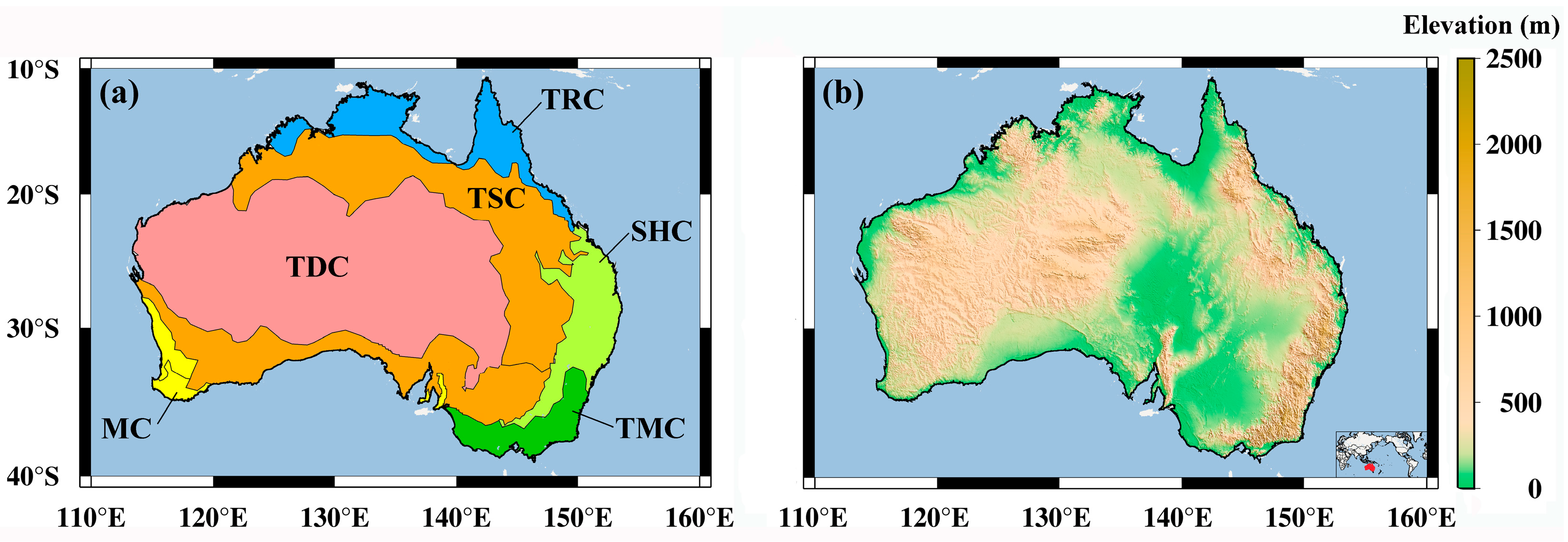
2. Study Area
3. Data and Method
3.1. Data
3.1.1. GRACE/GRACE-FO Data
3.1.2. Burned Area Data
3.1.3. In Situ Climate Data
3.1.4. Other Hydrometeorological Data
3.1.5. Standardized Precipitation Evapotranspiration Index Data
3.1.6. Extreme Climate Index Data
3.2. Method
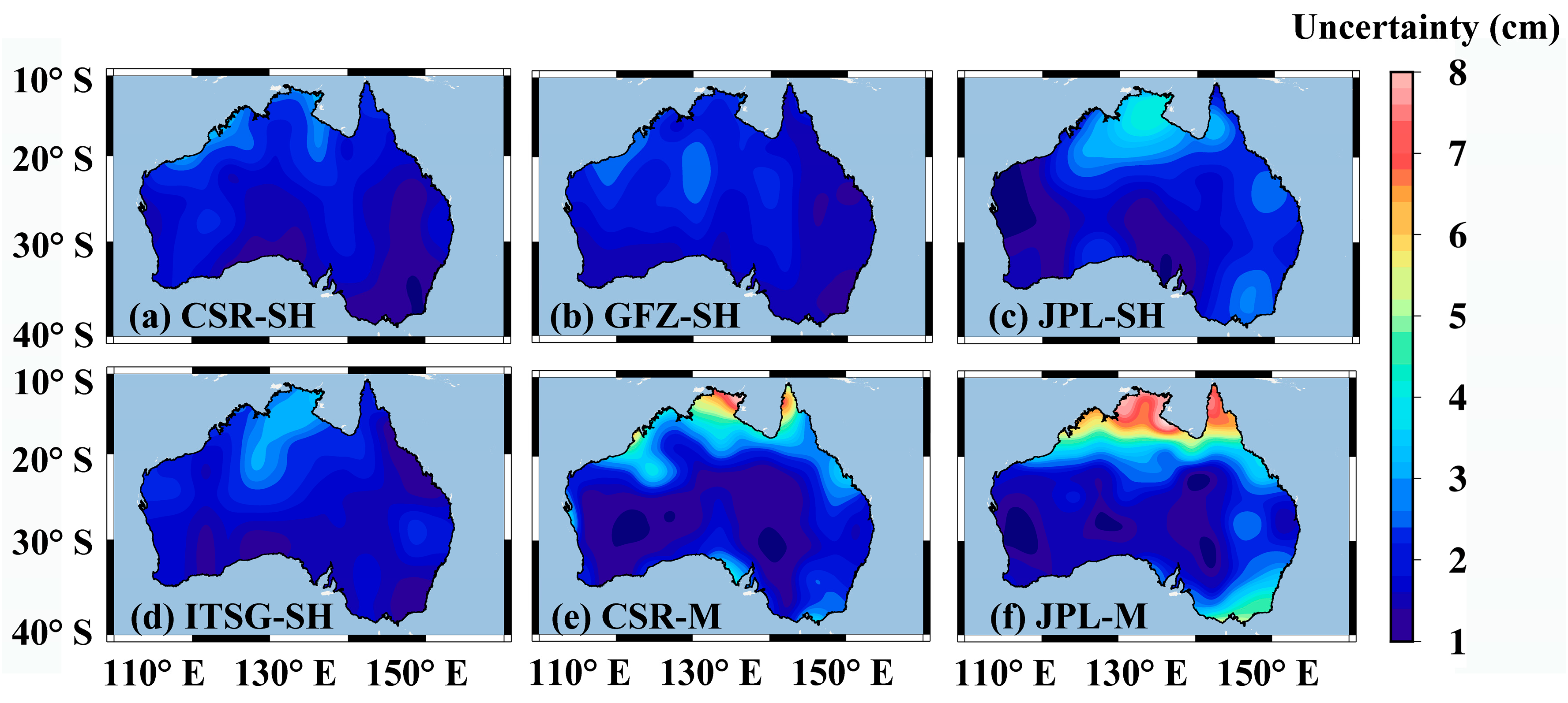
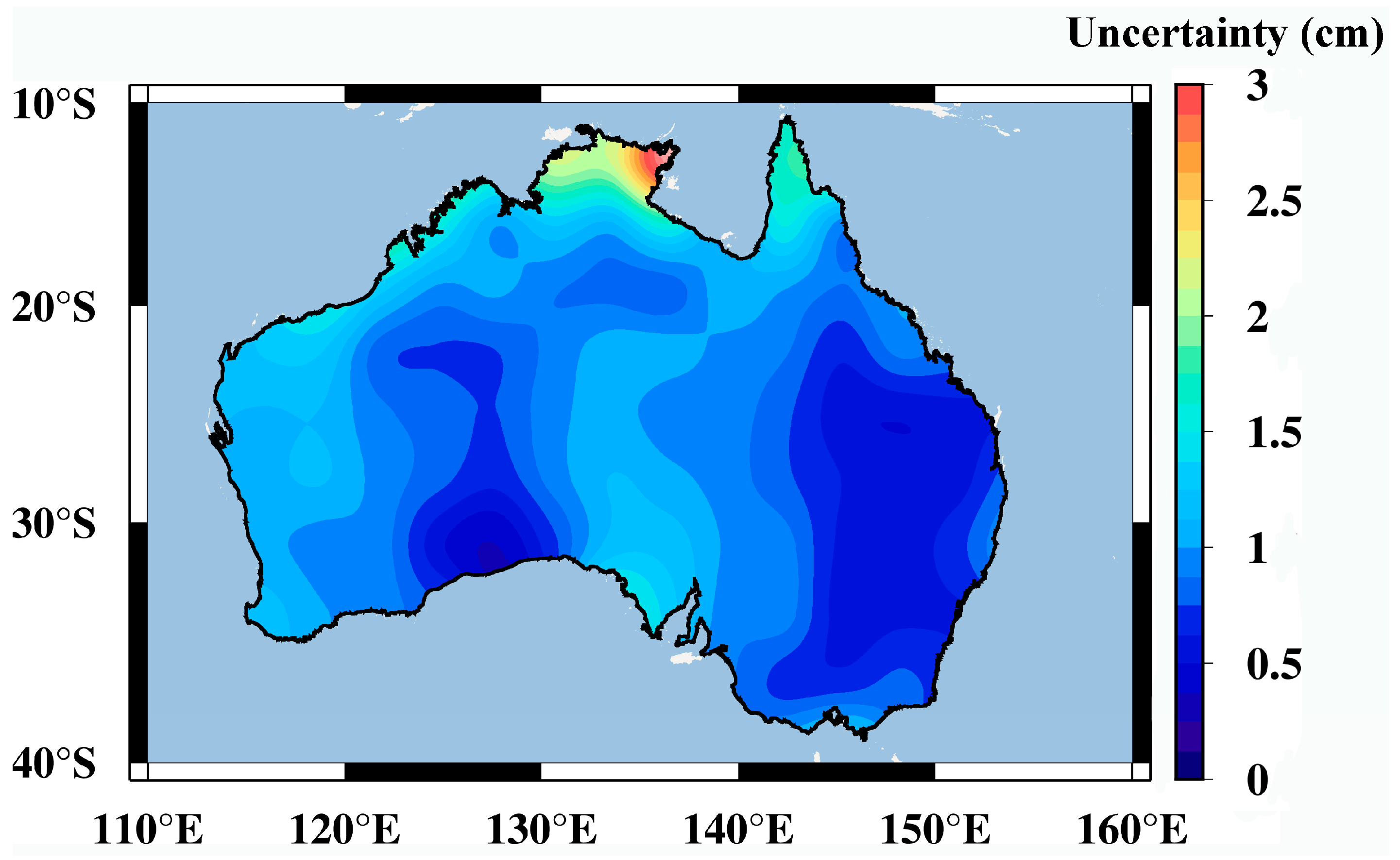
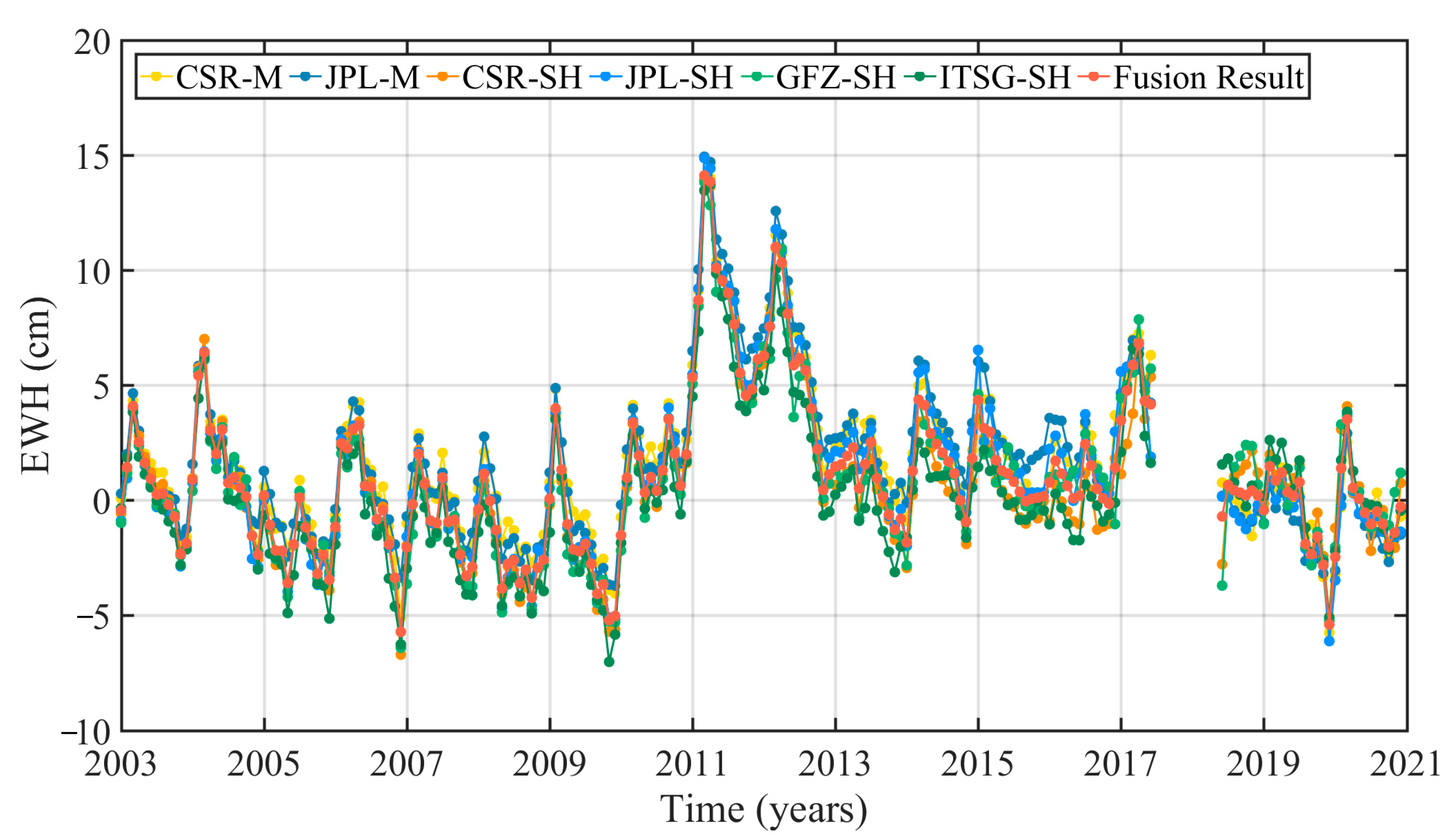
3.2.1. Data Fusion
3.2.2. GRACE-DSI
3.2.3. Composite Analysis
3.2.4. The Correlation Analysis and Delay Months
3.2.5. Nash–Sutcliffe Efficiency (NSE)
3.2.6. Standard Precipitation Index (SPI)
4. Results
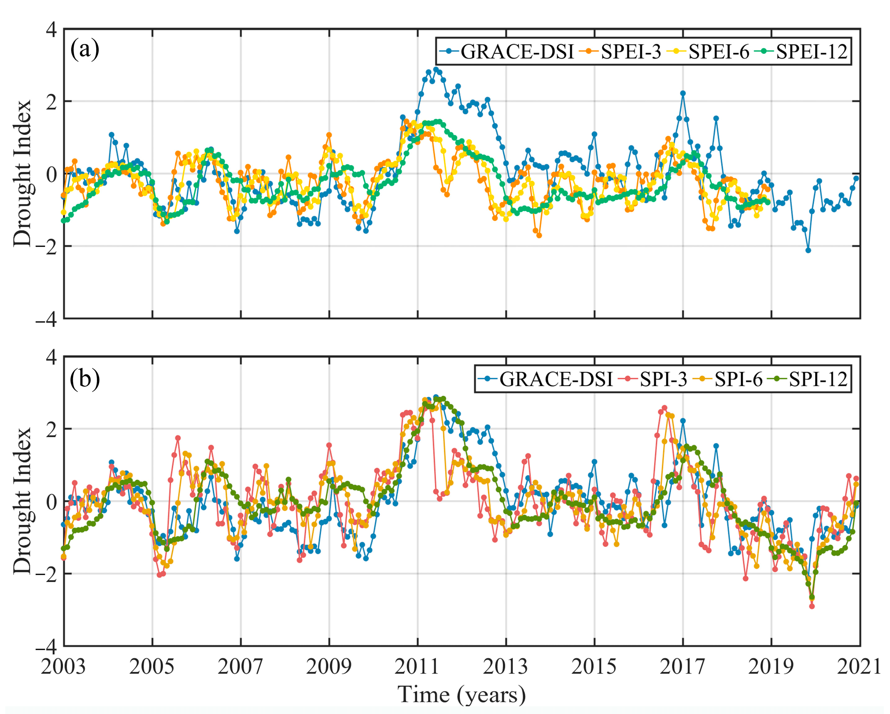
4.1. GRACE-DSI Construction
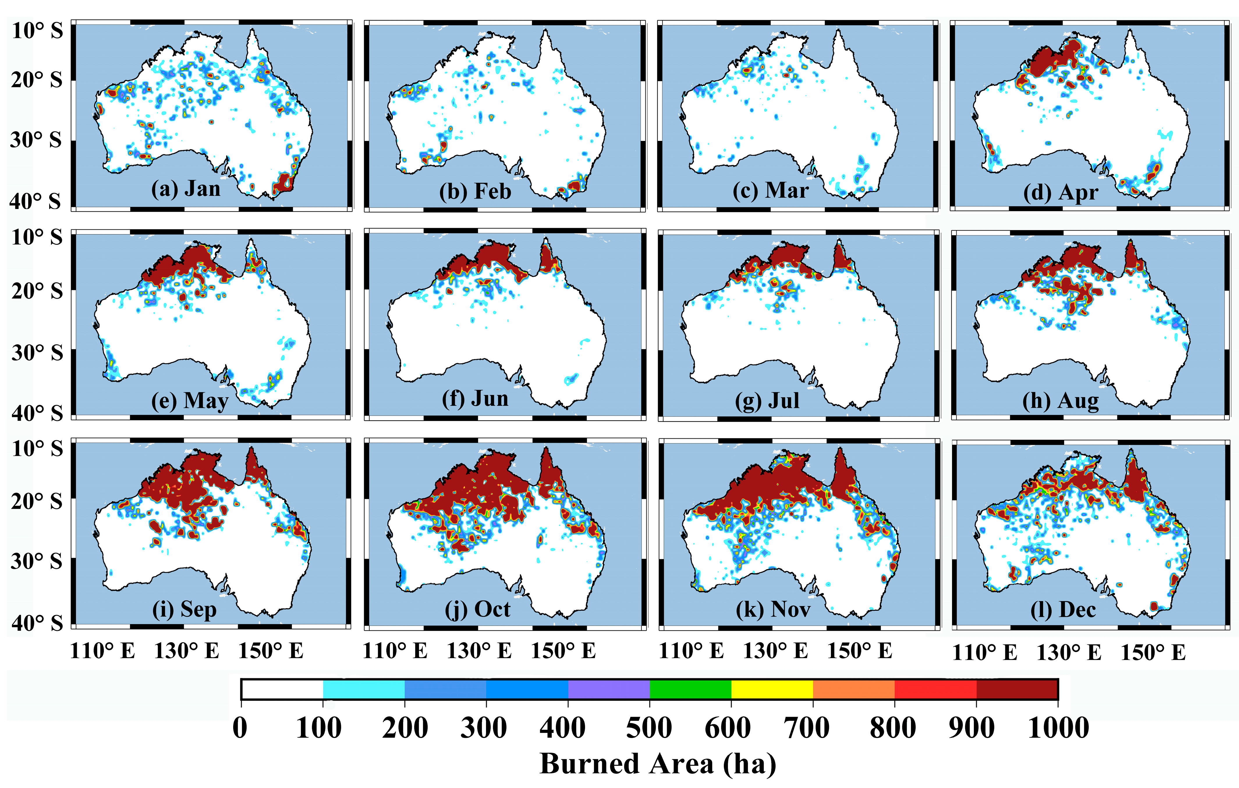
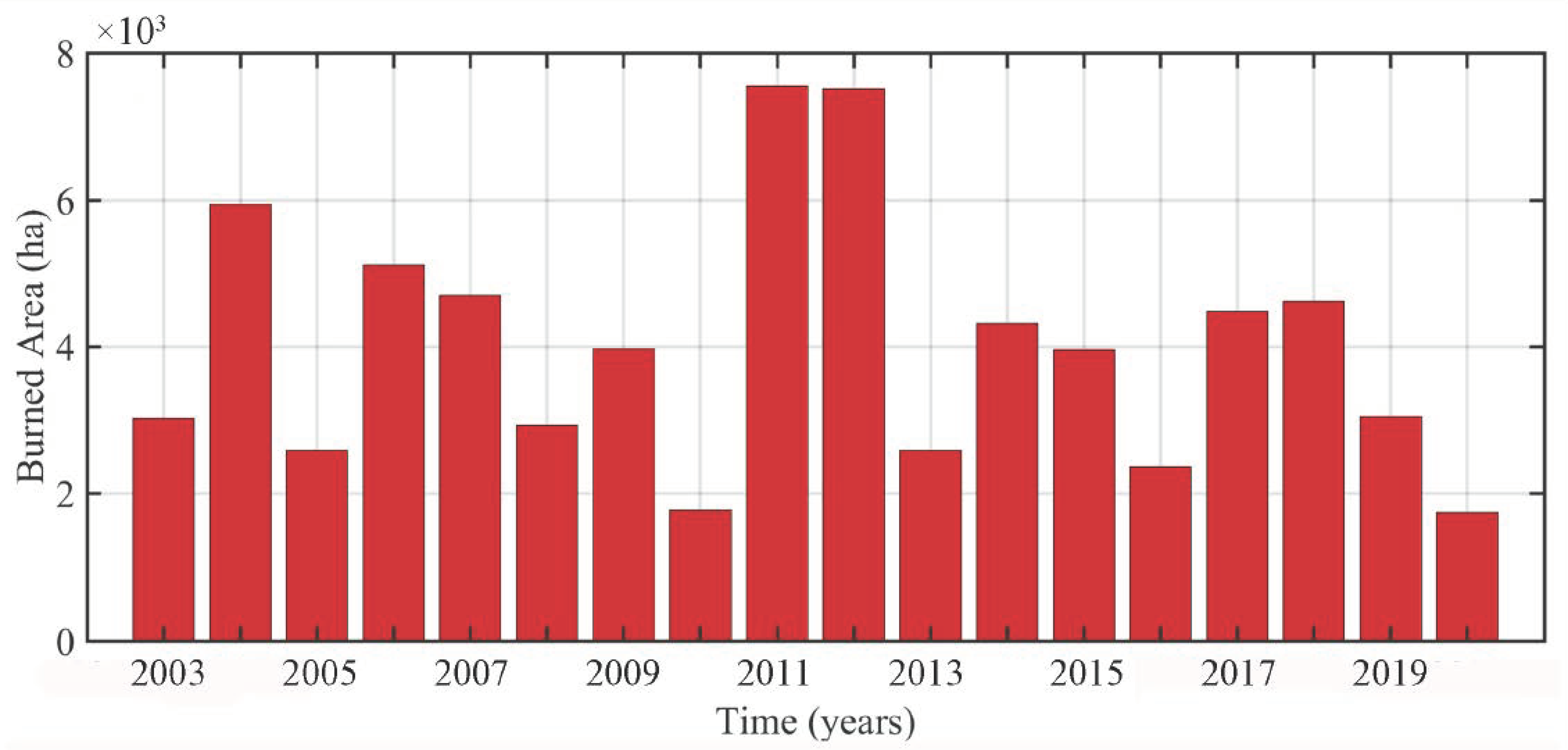
4.2. Spatiotemporal Distribution of Burned Area
4.3. The Connection between Hydrometeorological Factors and Wildfires
4.3.1. On a Seasonal Scale
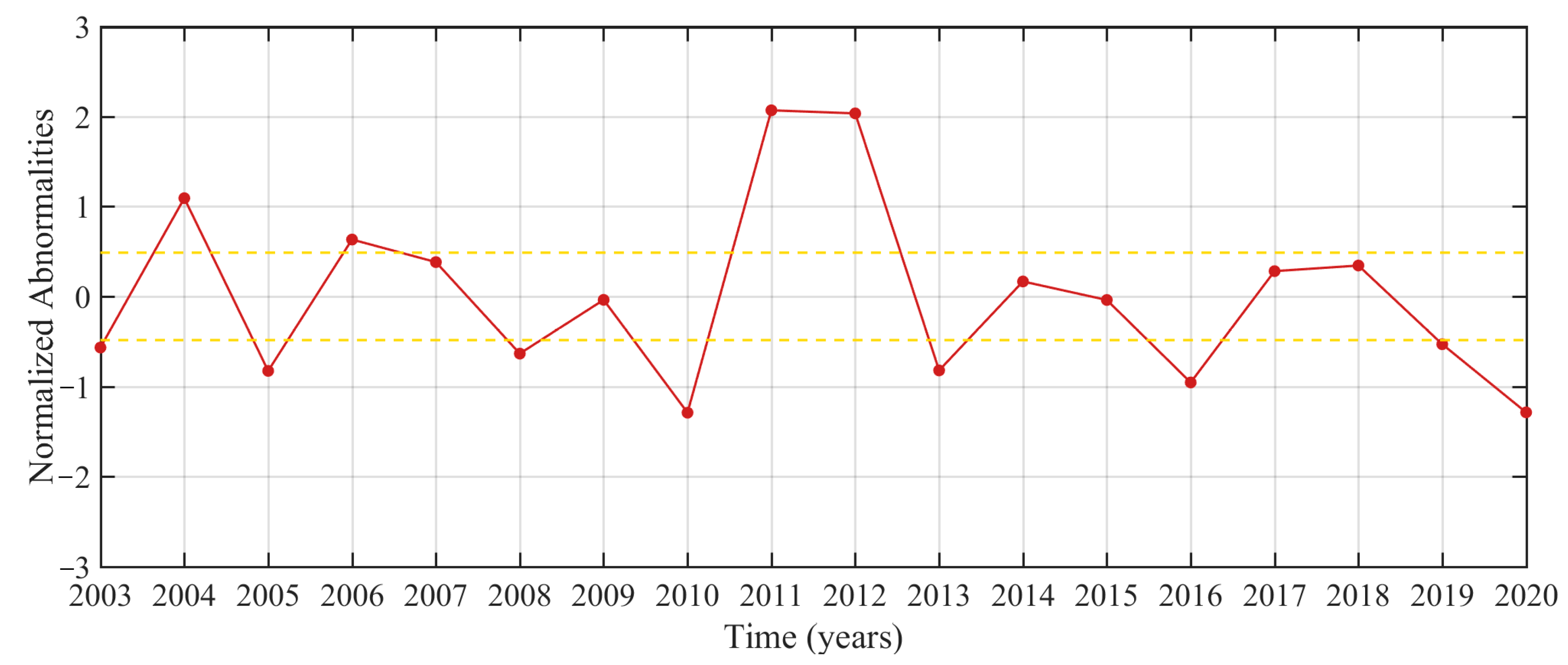
4.3.2. On an Interannual Scale
4.3.3. Performance of GRACE-DSI and Hydrometeorological Factors before Wildfire
5. Discussion
6. Conclusions
- (1)
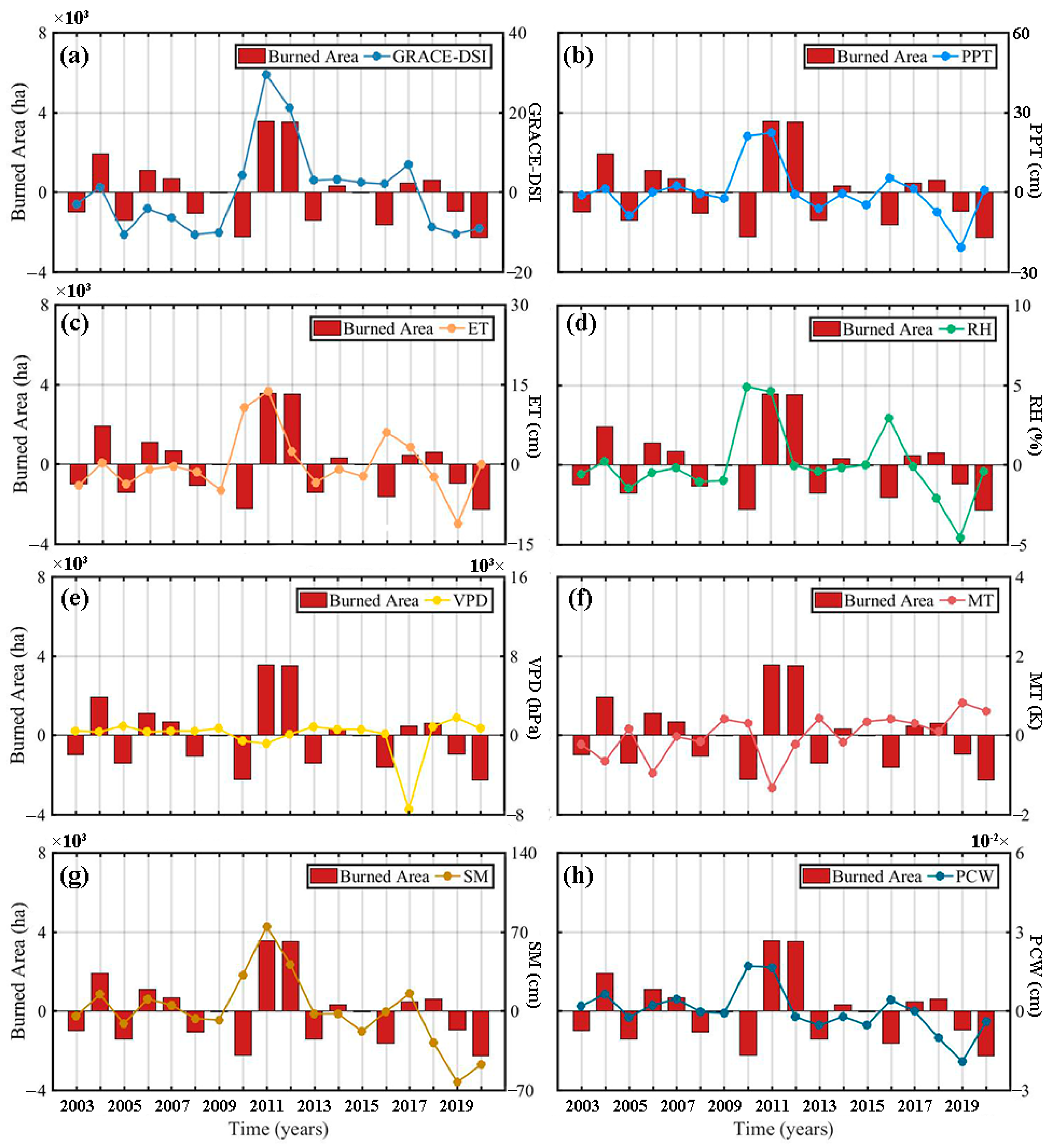
- In terms of spatial distribution, Australia’s wildfires are mainly concentrated in the north, with sporadic wildfires in the southeast. In terms of temporal distribution, Australia’s wildfires are mainly concentrated in October and November. In 2011 and 2012, two of Australia’s worst wildfires occurred during the 18-year study period.
- (2)
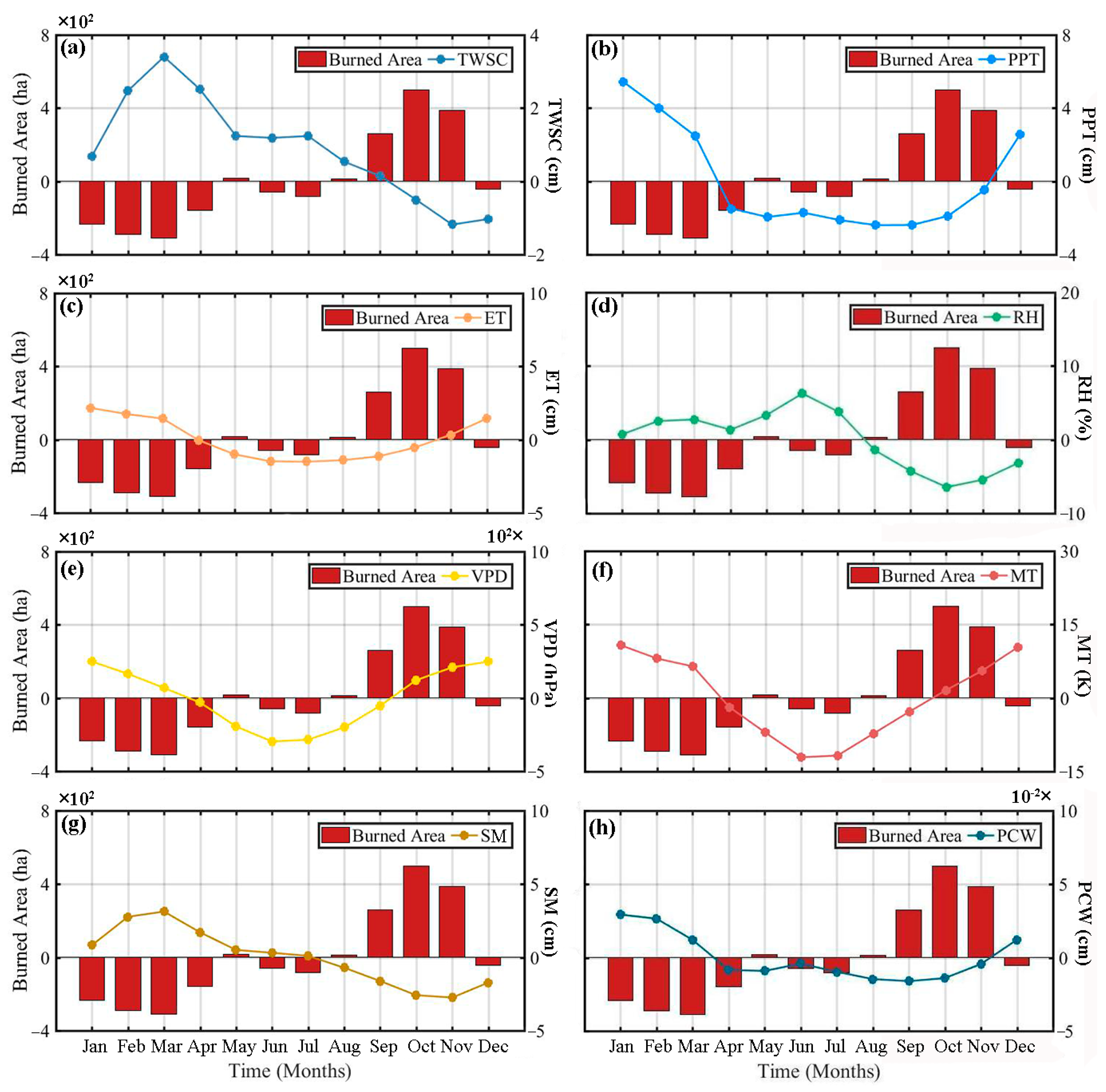
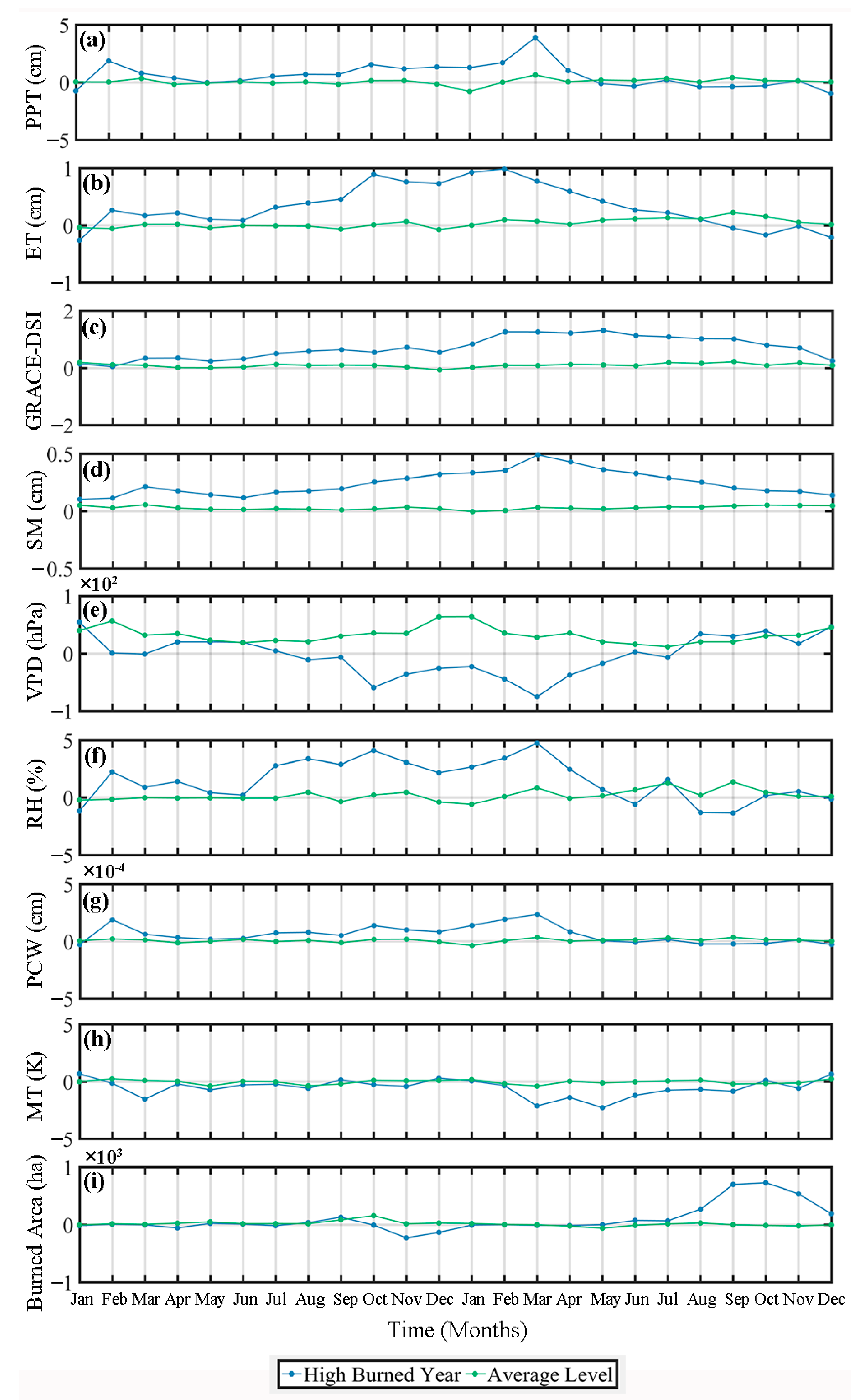
- TWSC and the seven hydrometeorological factors are strongly correlated with burned area on a seasonal scale. Before the occurrence of wildfires, the regional climate generally changes abnormally, especially during a high burned year.
- (3)
- Droughts often lead to an increased chance of wildfires, which not only provides an external environment that is easy for wildfires to occur, but also provides an accumulation of combustibles for the occurrence and spread of wildfires.
- (4)
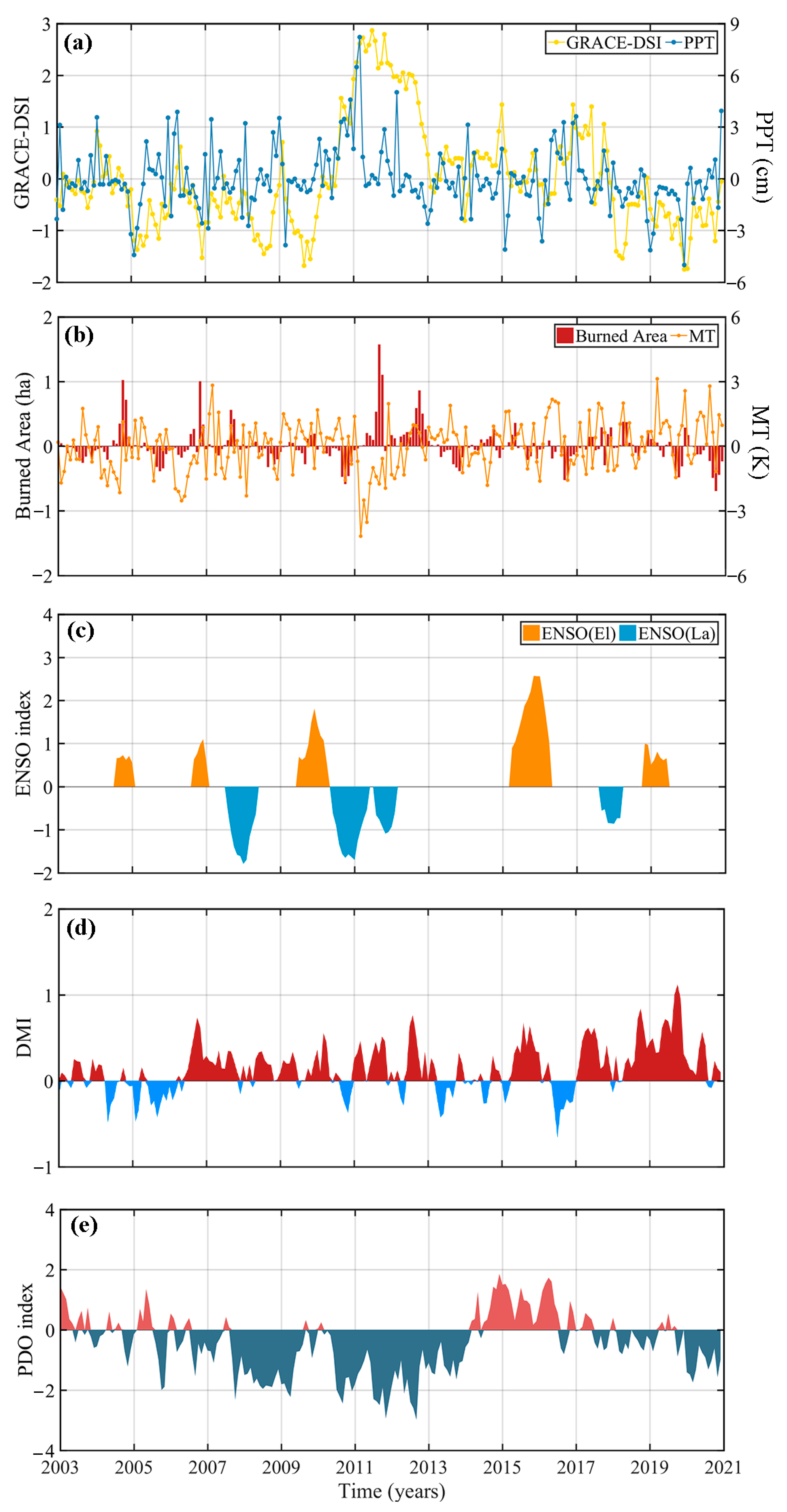
- An extreme climate event (ENSO, IOD, and PDO) is an important reason for the abnormal changes in regional climate, which has a strong influence on PPT and MT in Australia. An extreme climate event can lead to less PPT and higher MT, causing severe droughts.
- (5)
- The GRACE-DSI is a scientifically valid, easy-to-understand indicator of the occurrence and severity of droughts. Therefore, it can be used to evaluate the risk of wildfire occurrence.
Author Contributions
Funding
Institutional Review Board Statement
Informed Consent Statement
Data Availability Statement
Acknowledgments
Conflicts of Interest
References
- Goss, M.; Swain, D.; Abatzoglou, J.; Sarhadi, A.; Kolden, C.; Willams, A.; Diffenbaugh, N. Climate change is increasing the likehood of extreme autumn wildfires conditions across California. Environ. Res. Lett. 2020, 15, 094016. [Google Scholar] [CrossRef] [Green Version]
- Bradstock, R. A biogeographic model of fire regimes in Australia: Current and future implications. Glob. Ecol. Biogeogr. 2010, 19, 145–158. [Google Scholar] [CrossRef]
- van der Werf, G.R.; Randerson, J.T.; Giglio, L.; van Leeuwen, T.T.; Chen, Y.; Rogers, B.M.; Mu, M.; van Marle, M.J.E.; Morton, D.C.; Collatz, G.J.; et al. Global fire emissions estimates during 1997–2016. Earth Syst. Sci. Data 2017, 9, 697–720. [Google Scholar] [CrossRef] [Green Version]
- Ward, M.; Tulloch, A.; Radford, J.; Williams, B.; Reside, A.; Macdonald, S.; Mayfield, H.; Maron, M.; Possingham, H.; Vine, S.; et al. Impact of 2019–2020 mega-fires on Australian fauna habitat. Nat. Ecol. Evol. 2020, 4, 1321–1326. [Google Scholar] [CrossRef]
- Filkon, A.; Ngo, T.; Mattkews, S.; Telfer, S.; Penman, T. Impact of Australia’s catastrophic 2019/20 bushfire season on comminities and evvironment. Retrospective analysis and current trends. J. Safe. Sci. Resil. 2020, 1, 44–56. [Google Scholar]
- Arriagada, N.; Palmer, A.; Bowman, D.; Morgan, G.; Jalaludin, B.; Johnston, F. Unprecedented smoke-related health burden associated with the 2019-20 bushfires in eastern Australia. Med. J. Aust. 2020, 213, 282–283. [Google Scholar] [CrossRef]
- Dowdy, A.; Ye, H.; Pepler, A.; Thatcher, M.; Osbrough, S.; Evans, J.; Virgillio, G.; McCarthy, N. Futher changes in extreme weather and pyroconvection risk factors for Australian wildfires. Sci. Rep. 2019, 9, 10073. [Google Scholar] [CrossRef] [Green Version]
- Virgillio, G.; Evans, J.; Blake, S.; Armstrong, M.; Dowdy, A.; Sharples, J.; McRae, R. Climate change increases the potential for extreme wildfires. Geophys. Res. Lett. 2019, 46, 8517–8526. [Google Scholar] [CrossRef]
- Ehsani, M.R.; Arevalo, J.; Risanto, C.B.; Javadian, M.; Denine, C.J.; Arabzadeh, A.; Venegas-Quiñones, H.L.; Dell’Oro, A.P.; Behrangi, A. 2019–2020 Australia Fire and its relationship to hydroclimatological and vergetation variabilities. Water 2020, 12, 3067. [Google Scholar] [CrossRef]
- Flannigan, M.; Stocks, B.; Wotton, B. Climate change and forest fires. Sci. Total Environ. 2020, 262, 221–229. [Google Scholar] [CrossRef]
- Jolly, W.; Cochrane, M.; Freeborn, P.; Holden, Z.; Brown, T.; Williamson, G.; Bowman, D. Climate-induced variations in global wildfire danger from 1979 to 2013. Nat. Commun. 2015, 6, 7537. [Google Scholar] [CrossRef] [PubMed]
- Williams, A.; Karoly, D.; Tapper, N. The sensitivity of Australian fire danger to climate change. Cilm. Chang. 2001, 49, 171–191. [Google Scholar] [CrossRef]
- Westerling, L.; Gershunov, A.; Brown, T.; Cayan, D.; Dettinger, M. Climate and wildfire in the western United States. Bull. Amer. Meteorol. Soc. 2003, 84, 595–604. [Google Scholar] [CrossRef] [Green Version]
- Liu, Y.; Stanturf, J.; Goodrick, S. Trend in global wildfire potential in a changing climate. For. Ecol. Manag. 2010, 259, 685–697. [Google Scholar] [CrossRef]
- Piñol, J.; Terradas, J.; Lloret, F. Climate warming, wildfire hazard, and wildfire occurrence in coastal eastern Spain. Clim. Chang. 1998, 38, 345–357. [Google Scholar] [CrossRef]
- Nepstad, D.; Lefebvre, P.; Silva, U.; Tomasella, J.; Schlesinger, P.; Solorzano, L.; Moutinho, P.; Ray, D.; Benito, J. Amazon drought and its implications for forest flammability and tree growth: A basin-wide analysis. Glob. Chang. Biol. 2004, 10, 704–717. [Google Scholar] [CrossRef]
- Asner, G.; Alencar, A. Drought impacts on the Amazon Forest: The remote sensing perspective. New Phytol. 2010, 187, 569–578. [Google Scholar] [CrossRef]
- Roads, J.; Fujioka, F.; Chen, S.; Burgan, R. Seasonal fire danger forecasts for the USA. Int. J. Wildland Fire. 2005, 14, 1–18. [Google Scholar] [CrossRef]
- Collins, M.; Omi, P.; Chapman, P. Regional relationships between climate and wildfire burned area in the Interior West, USA. Can. J. Forest Res. 2006, 36, 699–709. [Google Scholar] [CrossRef]
- Preisler, K.; Westerling, A. Statistical model for forecasting monthly large forest fire events in western United States. J. Appl. Meteorol. Climatol. 2007, 46, 1010–1030. [Google Scholar] [CrossRef] [Green Version]
- Brando, P.; Nepstad, D.; Davidson, E.; Trumbore, S.; Ray, D.; Camargo, P. Drought effects on litterfall, wood production and belowground carbon cycling in an Amazon Forest: Results of a throughfall reduction experiment. Philos. Trans. R. Soc. B. Biol. Sci. 2008, 363, 1839–1848. [Google Scholar] [CrossRef]
- Chaparro, D.; Vall-Llossera, M.; Piles, M.; Camps, A.; Rüdiger, C.; Riera-Tatché, R. Predicting the extent of wildfires using remotely sensed soil moisture and temperature trends. IEEE J. Sel. Top. Appl. Earth Obs. Remote Sens. 2016, 9, 2818–2829. [Google Scholar] [CrossRef] [Green Version]
- Krueger, E.; Ochsner, T.; Carlson, J.; Engle, D.; Twidwell, D.; Fuhlendorf, S. Concurrent and antecedent soil moisture related positively or negatively to probability of large wildfire depending on season. Int. J. Wildland Fire 2016, 25, 657–668. [Google Scholar] [CrossRef]
- Jensen, D.; Reager, J.; Zajic, B.; Rousseau, N.; Rodell, M.; Hinkley, E. The sensitivity of US wildfire occurrence to pre-season soil moisture conditions across ecosystems. Environ. Res. Lett. 2018, 13, 014021. [Google Scholar] [CrossRef] [PubMed]
- Yu, G.; Wen, X.; Sun, X.; Tanner, B.; Lee, X.; Chen, J. Overview of China FLUX and evaluation of its eddy covariance measurement. Agric. For. Meteorol. 2006, 137, 125–137. [Google Scholar] [CrossRef]
- Cui, L.; Zhang, C.; Yao, C.; Luo, Z.; Wang, X.; Li, Q. Analysis of the influencing factors of drought events based on GRACE data under different climate conditions: A case study in Mainland China. Water 2021, 13, 2575. [Google Scholar] [CrossRef]
- Sun, Z.; Zhu, X.; Pan, Y.; Zhang, Y.; Zhang, J.; Liu, X. Drought evaluation using the GRACE terrestrial water storage deficit over the Yangtze River basin, China. Sic. Total Environ. 2018, 634, 727–738. [Google Scholar] [CrossRef]
- Ramillien, G.; Famiglietti, J.; Wahr, J. Detection of continental hydrology and glaciology signals from GRACE: A review. Surv. Geophys. 2008, 29, 361–374. [Google Scholar] [CrossRef] [Green Version]
- Chen, J.; Wilson, C.; Tapley, B.; Yang, Z.; Niu, G. 2005 drought event in the Amazon River basin as meatured by GRACE and estimated by climate model. J. Geophys. Res. 2009, 114, B05404. [Google Scholar]
- Frappart, F.; Paga, F.; da Silva, S.; Ramillien, G.; Prigent, C.; Seyler, F.; Calmant, S. Surface freshwater storage and dynamics in the Amazon basin during the 2005 exceptional drought. Environ. Res. Lett. 2012, 7, 44010. [Google Scholar] [CrossRef] [Green Version]
- Cui, L.; Zhang, C.; Luo, Z.; Wang, X.; Li, Q.; Liu, L. Using the local drought data and GRACE/GRACE-FO data to characterize the drought events in Mainland China from 2002 to 2020. Appl. Sci. 2021, 11, 9594. [Google Scholar] [CrossRef]
- Xie, Z.; Huete, A.; Restrepo-Coupe, N.; Ma, X.; Devadas, R.; Caprarelli, G. Spatial partitioning and temporal evolution of Australis’s total water storage under extreme hydroclimate impacts. Remote Sens. Environ. 2016, 183, 43–52. [Google Scholar] [CrossRef]
- Castle, S.; Thmas, B.; Reager, J.; Rodell, M.; Swenson, S.; Famiglietti, J. Groudwater depletion during drought threatens future water security of the Colorado River basin. Geophys Res. Lett. 2014, 41, 5904–5911. [Google Scholar] [CrossRef] [PubMed] [Green Version]
- Chen, Y.; Velicogna, I.; Famiglietti, J.; Randerson, J. Satellite observations of terrestrial water storage provide early warning information about drought and fire season severity in the Amazon. J. Geophys. Res. Biogeosci. 2013, 118, 495–504. [Google Scholar] [CrossRef] [Green Version]
- Farahmand, A.; Stavros, E.; Reager, J.; Behrangi, A.; Randerson, J.; Quayle, B. Satellite hydrology observations as operational indicators of forecasted fire danger across the contiguous United States. Nat. Hazards Earth Syst. Sci. 2020, 20, 1097–1106. [Google Scholar] [CrossRef] [Green Version]
- Cui, L.; Luo, C.; Yao, C.; Zou, Z.; Wu, G.; Li, Q.; Wang, X. The influence of climate change on forest fires in Yunnan province, Southwest China detected by GRACE satellite. Remote Sens. 2022, 14, 712. [Google Scholar] [CrossRef]
- Zink, M.; Samaniego, L.; Kumar, R.; Thober, S.; Mai, J.; Schäfer, D.; Marx, A. The German drought monitor. Environ. Res. Lett. 2016, 11, 074002. [Google Scholar] [CrossRef]
- Köppen, W. Die Wärmezonen der Erde, nach der Dauer der Heissen, Gemässigten, und Kalten Zeit, und nach der Wirkung der Wärme auf die Organisch Welt betrachtet. Meteorol. Z. 1884, 1, 215–226. Available online: http://www.metvis.com.au/acc/index.html (accessed on 22 February 2021).
- Herring, S.; Christidis, N.; Hoell, A.; Kossin, J.; Schreck III, C.; Stott, P. Explaining extreme events of 2016 from a climate perspective. Bull.Am. Meteorol. Soc. 2018, 99, S1–S157. [Google Scholar] [CrossRef] [Green Version]
- Swenson, S.; Chambers, D.; Whar, J. Estimating geocenter variations form a combination of GRACE and ocean model output. J. Geophys. Res. Solid Earth. 2008, 113, 194–205. [Google Scholar] [CrossRef] [Green Version]
- Cheng, M.; Tapley, B.D. Variations in the Earth’s oblateness during the past 28 years. J. Geophys. Res. 2004, 109, B09402. [Google Scholar] [CrossRef]
- Cui, L.; Yin, M.; Huang, Z.; Yao, C.; Wang, X.; Lin, X. The drought events over the Amazon River basin from 2003 to 2020 detected by GRACE/GRACE-FO and Swarm satellites. Remote Sens. 2022, 14, 2887. [Google Scholar] [CrossRef]
- Cui, L.; Song, Z.; Luo, Z.; Zhong, B.; Wang, X.; Zou, Z. Comparison of terrestrial water storage changes derived from GRACE/GRACE-FO and Swarm: A case study in the Amazon River Basin. Water 2020, 12, 3128. [Google Scholar] [CrossRef]
- Li, F.; Kusche, J.; Rietbroek, R.; Wang, Z.; Forootan, E.; Schulze, K.; Lück, C. Comparison of data-driven techniques to reconstruct (1992-2002) and Predict (2017-2018) GRACE-like gridded total water storage changes using climate inputs. Water Resour. Res. 2020, 56, WR026551. [Google Scholar] [CrossRef] [Green Version]
- Lizundia-Loiola, J.; Franquesa, M.; Khairoun, A.; Chuvieco, E. Global burned area mapping from Sentinel-3 Synergy and VIIRS active fires. Remote Sens Environ. 2022, 282, 113298. [Google Scholar] [CrossRef]
- Lizundia-Loiola, J.; Otón, G.; Ramo, R.; Chuvieco, E. A spatio-temporal active-fire clustering approach for global burned area mapping at 250m from MODIS data. Remote Sens. Environ. 2020, 236, 111493. [Google Scholar] [CrossRef]
- Schnelder, U.; Becker, A.; Finger, P.; Meyer-Christoffer, A.; Rudolf, B.; Ziese, M. GPCC full data reanalysis version 6.0 at 2.5°: Monthly land-surface precipitation from rain-gauges built on GTS-based and historic data. GPCC Data Rep. 2011, 10, 585. [Google Scholar]
- Miralles, D.; Holmes, T.; de Jeu, R.; Gash, H.; Meesters, A.; Dolman, A. Global land surface evaporation estimated from satellite-based observations. Hydrol. Earth Syst. Sci. 2011, 15, 453–469. [Google Scholar] [CrossRef] [Green Version]
- Rodell, M.; Houser, P.; Jambor, U.; Gottschalck, J.; Mitchell, K.; Meng, C.; Arsenault, K.; Cosgrove, B.; Radakovich, J.; Bosilovich, M.; et al. The Global Land Data Assimilation System. Bull. Am. Meteorol. Soc. 2004, 85, 381–394. [Google Scholar] [CrossRef] [Green Version]
- Vicente-Serrano, S.; Beguería, S.; López-Moreno, J. A multiscalar drought index sensitive to global warming: The standardized precipitation evapotranspiration index. J. Clim. 2010, 23, 1696–1718. [Google Scholar] [CrossRef] [Green Version]
- Mishra, A.; Singh, V. A review of drought concepts. J. Hydrol. 2010, 391, 202–216. [Google Scholar] [CrossRef]
- Mantua, N.; Hare, S.; Steven, R.; Zhang, Y.; Wallace, J.; Francis, R. A pacific interdecadal climate oscillation with impact on salmon production. Bull. Am. Meteorol. Soc. 1997, 78, 1069–1079. [Google Scholar] [CrossRef]
- Meyers, G.; Mcintosh, P.; Pigot, L.; Pook, M. The years of El Niño, La Niña and interactions with the Tropical Indian Ocean. J. Clim. 2007, 20, 2872–2880. [Google Scholar] [CrossRef]
- Ashok, K.; Guan, Z.; Yamagata, T. Impact of the Indian Ocean Dipole on the relationship between the Indian monsoon rainfall and ENSO. Geophys. Res. Lett. 2001, 28, 4499–4502. [Google Scholar] [CrossRef]
- Saji, N.; Goswami, B.; Vinayachandran, P.; Yamagate, T. A dipole model in the tropical Indian Ocean. Nature 1999, 401, 360–363. [Google Scholar] [CrossRef]
- Cui, L.; Zhu, C.; Wu, Y.; Yao, C.; Wang, X.; An, J.; Wei, P. Natural- and human- induced influences on terrestrial water storage change in Sichuan, Southwest China from 2003 to 2020. Remote Sens. 2022, 14, 1369. [Google Scholar] [CrossRef]
- Long, D.; Longuevergne, L.; Scanlon, B. Uncertainty in evapotranspiration from land surface modeling, remote sensing, and GRACE satellites. Water Resour. Res. 2014, 50, 1131–1151. [Google Scholar] [CrossRef] [Green Version]
- Zhao, Q.; Zhang, B.; Yao, Y.; Wu, W.; Chen, Q. Geodetic and htdrological measurements reveal the recent acceleration of groundwater depletion in North China Plain. J. Hydrol. 2019, 575, 1065–1072. [Google Scholar] [CrossRef]
- Long, D.; Pan, Y.; Zhou, J.; Chen, Y.; Hou, X.; Hong, Y.; Scanlon, B.; Longuevergne, L. Global analysis of spatiotemporal variability in merged total water storage changes using multiple GRACE products and global hydrological models. Remote Sens. Environ. 2017, 192, 198–216. [Google Scholar] [CrossRef]
- Chaudhari, S.; Pokhrel, Y.; Moran, E.; Miguez-Macho, G. Multi-decadal hydrologic change and variability in the Amazon River basin: Understanding terrestrial water storage variations and drought characteristics. Hydrol. Earth Syst. Sci. 2019, 23, 2841–2862. [Google Scholar] [CrossRef] [Green Version]
- Zhao, M.; Geruo, A.; Velicogna, I.; Kimball, J.S. A global gridded dataset of GRACE drought severity index for 2002-14: Comparison with PDSI and SPEI and a case study of the Australia. J. Hydrometeorol. 2017, 18, 2117–2129. [Google Scholar] [CrossRef] [Green Version]
- Eltahir, E.; Bras, R. Precipitation recycling. Rev. Geophys. 1996, 34, 367–378. [Google Scholar] [CrossRef]
- Lee, L.; Lawrence, D.; Price, M. Analysis of water-level response to rainfall and implications for recharge pathways in the Chalk aquifer, SE England. J. Hydrol. 2006, 330, 604–620. [Google Scholar] [CrossRef]
- Nash, J.; Sutcliffe, J. River flow forecasting through conceptual models part 1—A dicussion of pronciples. J. Hydrol. 1970, 10, 282–290. [Google Scholar] [CrossRef]
- Moriasi, D.; Arnold, J.; van Liew, M.; Bingner, R.; Harmel, R.; Veith, T. Model evalution guidelines for systematic quantification of accurary in watershed sumulation. Trans. ASABE 2007, 50, 885–900. [Google Scholar] [CrossRef]
- Werth, S.; Güntner, A.; Schmidt, R.; Kusche, J. Evaluation of GRACE filter tools from a hydrological perspective. Geophys. J. Int. 2009, 179, 1499–1515. [Google Scholar] [CrossRef] [Green Version]
- McKee, T.B.; Doesken, N.J.; Kleist, J. The relationship of drought frequency and duration to time scales. In Proceedings of the 8th Conference on Applied Climatology, Anaheim, CA, USA, 17–22 January 1993; pp. 179–184. [Google Scholar]
- Vicente-Serrano, S. Differences in spatial patterns of drought on different time scales: An analysis of the Iberian Peninsula. Water Resour. Manag. 2006, 20, 37–60. [Google Scholar] [CrossRef]
- Jipp, P.; Nepstad, D.; Cassel, D.; de Carvallo, C. Deep soil moisture storage and transpiration in forests and pastures of seasonally-dry Amazonia. Clim. Chang. 1998, 39, 395–412. [Google Scholar] [CrossRef]
- Fernandes, K.; Baethgen, W.; Bernardes, S.; Defries, R.; Dewitt, D.; Goddard, L.; Lavado, W.; Lee, D.; Padoch, C.; Pinedo-Vasques, M.; et al. North Tropical Atlantic influence on western Amazon fire season variability. Geophys. Res. Lett. 2011, 38, L12701. [Google Scholar] [CrossRef] [Green Version]
- Annamalai, H.; Kida, S.; Hanfner, J. Potential impact of the tropical Indian Ocean-Indonesian Seas on El Niño characteristics. J. Clim. 2010, 23, 3933–3952. [Google Scholar] [CrossRef]
- Aragon, L.; Malhi, Y.; Roman-Cuesta, R.; Saatchi, S.; Anderson, L.; Shimabukuro, Y. Spatial patterns and fire response of recent Amazonian droughts. Geophys. Res. Lett. 2007, 34, L07701. [Google Scholar]
- Cui, L.; He, M.; Zou, Z.; Yao, C.; Wang, S.; An, J.; Wang, X. The influence of climate change on Droughts and floods in the Yangtze River basin from 2003 to 2020. Sensors 2022, 22, 8178. [Google Scholar] [CrossRef] [PubMed]


| Type | GRACE-DSI | Type | GRACE-DSI |
|---|---|---|---|
| Exceptional Drought | Moderate Drought | −1.3~−0.8 | |
| Extreme Drought | −2.0~−1.6 | Light Drought | −0.8~−0.5 |
| Severe Drought | −1.6~−1.3 | No Drought |
| Variables | Correlation Coefficients | Lag Months | ||
|---|---|---|---|---|
| High Burned Year | Average Level | High Burned Year | Average Level | |
| PPT vs. GRACE-DSI | 0.52 | 0.50 | 4 | 1 |
| ET vs. GRACE-DSI | 0.90 | 0.52 | 4 | 2 |
| GRACE-DSI vs. Burned Area | −0.50 | −0.32 | 4 | 2 |
| PPT vs. SM | 0.67 | 0.50 | 1 | 1 |
| ET vs. SM | 0.87 | 0.81 | 2 | 4 |
| GRACE-DSI vs. SM | 0.86 | 0.71 | 1 | 2 |
| ET vs. VPD | −0.92 | −0.51 | 0 | 4 |
| ET vs. RH | 0.82 | 0.79 | 0 | 4 |
| SM vs. PCW | 0.67 | 0.62 | 0 | 1 |
| GRACE-DSI vs. VPD | −0.83 | −0.46 | 4 | 2 |
| GRACE-DSI vs. RH | 0.65 | 0.49 | 4 | 1 |
| GRACE-DSI vs. PCW | 0.50 | 0.49 | 4 | 2 |
| GRACE-DSI vs. MT | −0.61 | −0.36 | 0 | 2 |
| VPD vs. Burned Area | 0.59 | 0.74 | 1 | 3 |
| RH vs. Burned Area | −0.62 | −0.51 | 1 | 3 |
| PCW vs. Burned Area | −0.59 | −0.58 | 1 | 3 |
| MT vs. Burned Area | 0.73 | 0.10 | 4 | 3 |
| Variables | Correlation Coefficients | Lag Months |
|---|---|---|
| ENSO vs. PPT | −0.56 | 2 |
| ENSO vs. MT | 0.57 | 4 |
| ENSO vs. GRACE-DSI | −0.33 | 3 |
| ENSO vs. Burned area | 0.13 | 5 |
| DMI vs. PPT | −0.42 | 2 |
| DMI vs. MT | 0.47 | 6 |
| DMI vs. GRACE-DSI | −0.23 | 5 |
| DMI vs. Burned area | 0.25 | 1 |
| POD vs. PPT | −0.45 | 5 |
| POD vs. MT | 0.35 | 4 |
| POD vs. GRACE-DSI | −0.31 | 2 |
| POD vs. Burned area | 0.18 | 5 |
Disclaimer/Publisher’s Note: The statements, opinions and data contained in all publications are solely those of the individual author(s) and contributor(s) and not of MDPI and/or the editor(s). MDPI and/or the editor(s) disclaim responsibility for any injury to people or property resulting from any ideas, methods, instructions or products referred to in the content. |
© 2023 by the authors. Licensee MDPI, Basel, Switzerland. This article is an open access article distributed under the terms and conditions of the Creative Commons Attribution (CC BY) license (https://creativecommons.org/licenses/by/4.0/).
Share and Cite
Cui, L.; Zhu, C.; Zou, Z.; Yao, C.; Zhang, C.; Li, Y. The Spatiotemporal Characteristics of Wildfires across Australia and Their Connections to Extreme Climate Based on a Combined Hydrological Drought Index. Fire 2023, 6, 42. https://doi.org/10.3390/fire6020042
Cui L, Zhu C, Zou Z, Yao C, Zhang C, Li Y. The Spatiotemporal Characteristics of Wildfires across Australia and Their Connections to Extreme Climate Based on a Combined Hydrological Drought Index. Fire. 2023; 6(2):42. https://doi.org/10.3390/fire6020042
Chicago/Turabian StyleCui, Lilu, Chengkang Zhu, Zhengbo Zou, Chaolong Yao, Cheng Zhang, and Yu Li. 2023. "The Spatiotemporal Characteristics of Wildfires across Australia and Their Connections to Extreme Climate Based on a Combined Hydrological Drought Index" Fire 6, no. 2: 42. https://doi.org/10.3390/fire6020042