Remote Sensing Applications for Mapping Large Wildfires Based on Machine Learning and Time Series in Northwestern Portugal

Abstract

Mapping large wildfires (LW) is essential for environmental applications and enhances the understanding of the dynamics of affected areas. Remote sensing techniques supported by machine learning and time series have been increasingly used in studies addressing this issue and have shown potential for this type of analysis. The main aim of this article is to develop a methodology for mapping LW in northwestern Portugal using a machine learning algorithm and time series from Landsat images. For the burnt area classification, we initially used the Fourier harmonic model to define outliers in the time series that represented pixels of possible burnt areas and, then, we applied the random forest classifier for the LW classification. The results indicate that the harmonic analysis provided estimates with the actual observed values of the NBR index; thus, the pixels classified by random forest were only those that were masked, collaborated in the processing, and reduced possible spectral confusion between targets with similar behaviour. The burnt area maps revealed that ~23.5% of the territory was burnt at least once from 2001 to 2020. The temporal variability of the burnt area indicated that, on average, 6.504 hectares were affected by LW within the 20 years. The annual burnt area varied over the years, with the minimum annual area detected in 2014 (679.5 hectares) and the maximum mapped area detected in 2005 (73,025.1 hectares). We concluded that the process of defining the mask with the outliers considerably reduced the universe of pixels to be classified within each image, which leaves the training of the classifier focused on separating the set of pixels into two groups with very similar spectral characteristics, thus contributing so that the separation of groups with similar spectral behaviour was performed automatically and without great sampling effort. The method showed satisfactory accuracy results with little omission for burnt areas.

1. Introduction

In recent decades, large wildfires (LW) have caused severe short- and long-term disruptions to ecosystems, biodiversity, human health, and infrastructure throughout the world [1,2,3,4,5,6], and they constitute an important research topic, due to the multiplicity of effects they can have on society and on the environment [7,8]. Although fires are an ancient phenomenon and play an ecological role in some ecosystems [9,10,11], fire regimes have been changing in many regions of the world because of the effects of increasing temperature and reduced precipitation, and, in this sense, the impacts of human activities cannot be underestimated [3,10,12].

Europe has registered a high number of fires and an extensive burnt area in the last decades with different spatial and temporal trends [13,14,15,16]. The Mediterranean region has favourable environmental conditions for fires to occur, which contribute to a high rate of wildfires [6,17], and their size has increased significantly [4,6,12,18,19]. Given this reality, Portugal is one of the European countries most affected by fires [14,20,21]. Despite its smaller land area compared to other Mediterranean countries [22,23,24], it is found to be one of the most fire-prone countries in southern Europe [6].

Historically, wildfires are one of Portugal’s most significant drivers for land use and land cover changes [25,26]. However, over time we have observed a new reality in the country regarding large wildfires (LW) [27], which are considered, in this work, as any fire that covers an area larger than 100 ha [28], which has been believed to be one of the most significant sources of degradation of an important part of its territory.

For this reason, it is essential to develop studies that seek to comprehend wildfire dynamics. This society’s concern has had, as a beneficial consequence, the development of more efficient tools that enhance the understanding of this problem.

Since the late 1970s, satellite-based remote sensing data have been widely used to detect active wildfires and map burnt areas [7,29,30]. Landsat archives provide frequent Earth surface reflectance data from ~1984 with a spatial resolution (~30m) that is useful for characterizing burnt areas [31]. This type of data makes it possible to estimate the extent of the fire, the affected area, and the burn severity at different scales owing to its temporal, spatial, and spectral resolutions [32]. Mapping the burnt area can broaden the knowledge of the dynamics of the areas affected by fires worldwide [7,30], mainly because of the possibility of data analysis based on time series [33,34,35,36].

Spectral indices are typically employed to derive vegetation properties from remote sensing data [37]. For research on areas affected by wildfires, vegetation indices are commonly founded on radiometric measurements taken before and after a fire or simulated by an energy transfer model [37]. Nevertheless, one should bear in mind that, in a burnt area, there is a wide range of fire severity and, therefore, a large variety of spectral mixtures among charcoal, ash, soil, and burnt vegetation.

Moreover, spectral indices usually combine information from the visible, near-infrared, and mid-infrared (SWIR) portions of the electromagnetic spectrum [38,39,40]. These bands are sensitive to variations in soil colour (visible and mid-infrared), soil composition (mid-infrared), moisture, and chlorophyll (near-infrared), which are all properties of land and vegetation that can be significantly affected by fire [38]. Several authors have shown that the SWIR range (1200–2400 nm) provides a clearer separation of burnt areas [41].

Lately, machine learning techniques (ML) have been applied for the development of studies addressing this issue. ML is an effective empirical approach that can be used in remote sensing applications, such as the supervised classification of satellite images [42]. Its major focus is to automatically extract information from data by computational and statistical methods [43,44,45]. ML algorithms are highly useful, as they are “universal approximators” that can learn the behaviour of a system if they are given a broad set of examples in a training dataset.

These examples should cover as much of the parameter space as possible and are non-parametric, non-linear, and multivariate learning algorithms [42,43]. Algorithms based on random forest (RF) methods are frequently used [46,47,48,49,50] in ML applications, given that they are a non-parametric supervised method applied both for classification and prediction [12]. Studies in this perspective were developed by [1,3,12,31,33,51]. In this context, in this study, we have proposed an approach to improve the existing methodologies based on ML, which is intended to achieve a more automated process using the RF method, which allows for the classification of wildfires with estimated values and reduces possible classification errors. The main aim of this article is to develop a methodology for mapping LW in northwestern Portugal using a machine learning algorithm and time series from Landsat images.

2. Materials and Methods

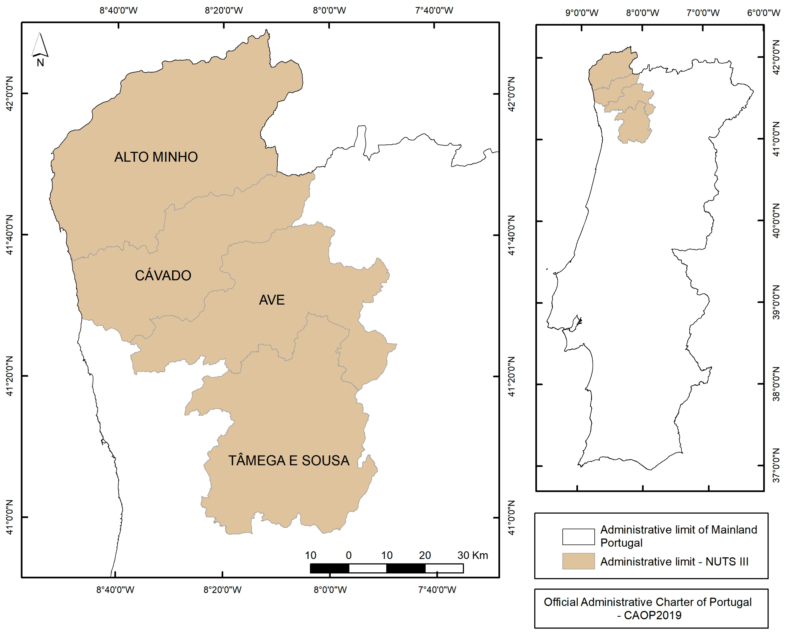
2.1. Study Area

The study was undertaken in 4 territorial units of level III (NUTSIII) located in northwestern Portugal, namely Alto Minho, Cávado, Ave, and Tâmega e Sousa (Figure 1), which correspond to a territorial area of approximately 6.748 km².

With respect to physical characteristics, this territory has very specific features, either in terms of relief configurations and associated hydromorphological dynamics or from the viewpoint of climatic and vegetation distribution, that build quite a peculiar landscape and intersect with a very distinctive anthropic occupation, which distinguish it from the rest of the national territory, largely due to the existing physical conditioning [52,53,54].

The northwest has frequently suffered from a significant number of wildfires [53]. Its natural characteristics, such as the predominant vegetation type as well as the climatic conditions, favour the occurrence of fires. The climate has Mediterranean traits, which are classified by the Köppen criteria as a Csb, that is, a mesothermal climate with a dry summer.

Climate influences acting chiefly on the quantity and type of vegetation in the region, as well as on the seasonal dynamics of its moisture content, act directly and indirectly upon the occurrence of forest fires and their propagation. The high rainfall regime registered in the northwest, with averages above 2000 mm, allows for a high biomass productivity, which makes municipalities where wild spaces have greater territorial expression more vulnerable to the occurrence of fire, particularly the most mountainous ones [52].

Fire occurrences in mainland Portugal normally happen between July and September, with summer as a critical period. However, it has been increasingly observed that large fires have taken place between June and October [55]. The key factors causing the conditions of large wildfires to occur are high temperatures above 35/40 °C, dry air with humidity below 25%, and the joint flow of Atlantic or European anticyclones [28,56,57].

In these conditions of favourable atmospheric dynamics, especially in summer months, such as under the influence of heat waves and meteorological droughts [57] with low pressure cores, higher temperatures connected with lower values of relative humidity are observed, which create more critical situations that lead to greater risks of wildfires in the country [28].

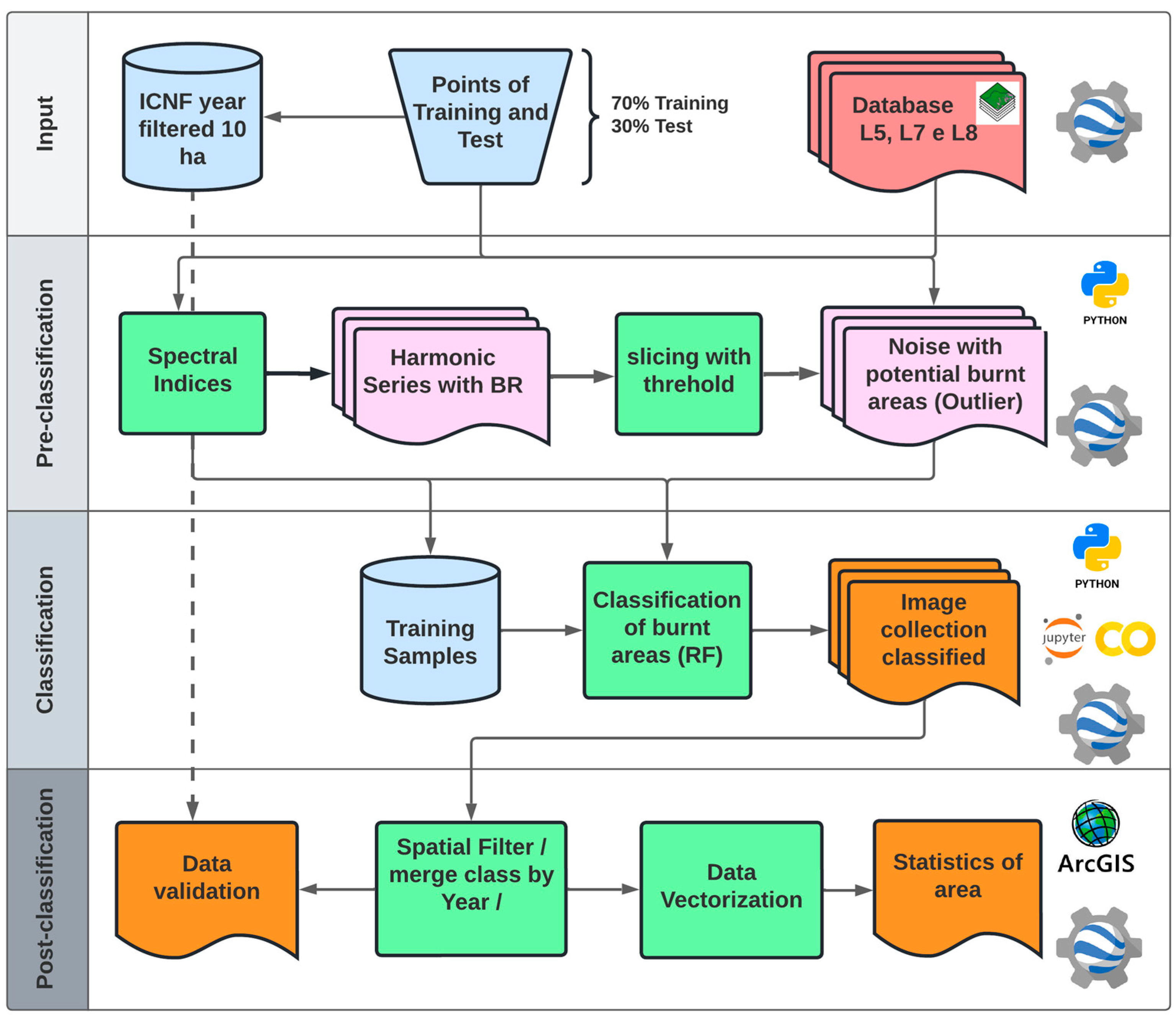
2.2. Burned Area Classification Approach

Figure 2 depicts our methodological approach for mapping burnt areas in northwestern Portugal. The steps are detailed in the following sub-topics.

2.2.1. Dataset

In this study, we used the Landsat surface reflectance (SR) dataset (30 m of the resolution, level 2, collection 2, tier 1) from 2001 to 2020. This dataset contains atmospherically corrected surface reflectance. We used the 232 available scenes for path/row 204/031 with cloud cover below 70% for Landsat 5, 7, and 8 (sensor thematic mapper (TM) for Landsat 5, enhanced thematic mapper plus (ETM+) for Landsat 7, and the operational land imager (OLI) for Landsat 8, available on the Google Earth Engine (GEE) platform), all with 16 days of temporal resolution and 30 m of spatial resolution. Figure 3 shows the distribution of images by sensor and year.

To address the problems related to pixel contamination by clouds and cloud shadow present in the image, we used the quality assessment band ‘pixel_qa’ of each image in the series (BQA 16 Bits), which was generated from the CFMask algorithm [58,59,60].

This band is constructed from the CFMask algorithm and facilitates the removal of pixels with clouds, shadow, and snow, since they are already classified in this band as the post-processing of the image. This method is based on the detection of abrupt spectral changes along the series, under the assumption that the images in time follow smooth variations, and the abrupt changes will be mainly due to the presence of clouds. We used a linear and non-linear regression algorithm that simultaneously minimized the prediction and estimated error. Then, the clouds were identified with the difference between the image of interest and the estimated image. The non-linear regression uses a kernel method that makes it possible to estimate the function of order greater than 1. We applied permissive rules, and only pixels with high confidence levels of “cloud”, “shadow”, and “radiometric saturation” were masked [59,60]. We used a statistical approach per year to summarize this amount of data and optimize the classification without discarding the spectral information about each pixel.

In addition to the satellite imagery, we handled data referring to the burnt areas from 2001 to 2020, which were provided by the Institute for the Conservation of Nature and Forests (ICNF), and the administrative limits of mainland Portugal were provided by the Directorate General for Territory (DGT).

Typology and Definition of Classes

The definition of elements for classification was organized into two categories: superclasses and subclasses. At the first level of abstraction of classes presented in the images, we opted to group different features into two superclasses: Burnt areas and Unburnt areas. At the second level, we identified subclasses and categorized them to understand the study area and collect samples for classification.

Table 1. Definition of the typologies of classes present in the images.

Superclasses	Subclasses	Tipology	Description
Burnt area (by different intensities)	Burnt area scenario 01		Areas characterized by recent fires with soil exposure in different types of vegetation.
	Burnt area scenario 02
	Burnt area scenario 03
Unburnt area	Vegetation		Category that includes vegetation types composed of forests and non-forest natural formations, including forestry areas.
	Non-vegetated area (bare rock)		Mixed class that includes agricultural areas in preparation, exposed soil, rocky outcrops, and sandy surfaces.
	Non-vegetated area (exposed soil)
	Surface Water		Surface water bodies that can be continuous (e.g., rivers and lakes) or isolated (e.g., flooded areas and dams).
	Cloud/Cloud Shadow/Relief Shadow		Features identified in the image as cloud, cloud shadow, and relief shadow.
	Urban infrastructure		Class that includes urban and industrial areas.

presents both categories of classes, their typologies, and their descriptions.

2.2.2. Pre-Classification

Spectral Indices

After literature review, several spectral indices were included and tested based on their performance for the study area. We tested 8 spectral indices (

Table 2. Spectral indices for evaluation of the burnt area. The delta version of each index as the difference between pre- and post-fire values was tested in this study.

Spectral Index	Formula
Normalized Burn Ratio (NBR) [65]	$R_{NIR}-R_{SWIR2}/R_{NIR}+R_{SWIR2}$
Mid Infrared Burn Index (MIRBI) [66]	$10R_{SWIR1}-9.8R_{SWIR2}+2$
Burned Area Index (BAI) [37]	$1/{\left(0.06-R_{NIR}\right)}^2+{\left(0.06-R_{RED}\right)}^2$
Normalized Difference Vegetation Index (NDVI) [67]	$\left(R_{NIR}-R_{RED}\right)/\left(R_{NIR}+R_{RED}\right)$
Enhanced Vegetation Index (EVI) [68]	$\frac{2.5(R_{NiR}-R_{RED})}{R_{NIR}}+6R_{RED}-7.5R_{BLUE}+1$
Normalized Difference Moisture Index (NDMI) [69]	$(R_{NIR}-R_{SWIR1})/(R_{NIR}+R_{SWIR1})$
Soil Adjusted Vegetation Index (SAVI) [70]	$(1+L)(R_{NIR}-R_{RED})/R_{NIR}+R_{RED}+L)$
Green Normalized Difference Vegetation Index (GNDVI) [71]	$\left(R_{NIR}-R_{GREEN}\right)/\left(R_{NIR}+R_{GREEN}\right)$
Difference (dNDVI; dNBR; dMIRBi; dNIR)	$Di{f}_{pre}-Di{f}_{post}$

), 5 bands (“red”, “blue”, “green”, “nir”, “swir1”), and the temporal differences of the NBR, MIRBI, NDVI, and the NIR band (delta versions which calculate the change between pre-fire and post-fire spectral index values) that are typically employed to assess fire severity. Although there is an extensive literature on fire mapping indices, we selected the commonly used indices to test our hypothesis [38,41]. These indices were calculated for each of the time series images [8,37,38,40,61,62,63,64] using a combination of Landsat 5 and 7 TM [“B1”, “B2”, “B3”, “B4”, “B5”, “B7”] and 8 OLI [“B2”, “B3”, “B4”, “B5”, “B6”, “B7”] spectral bands.

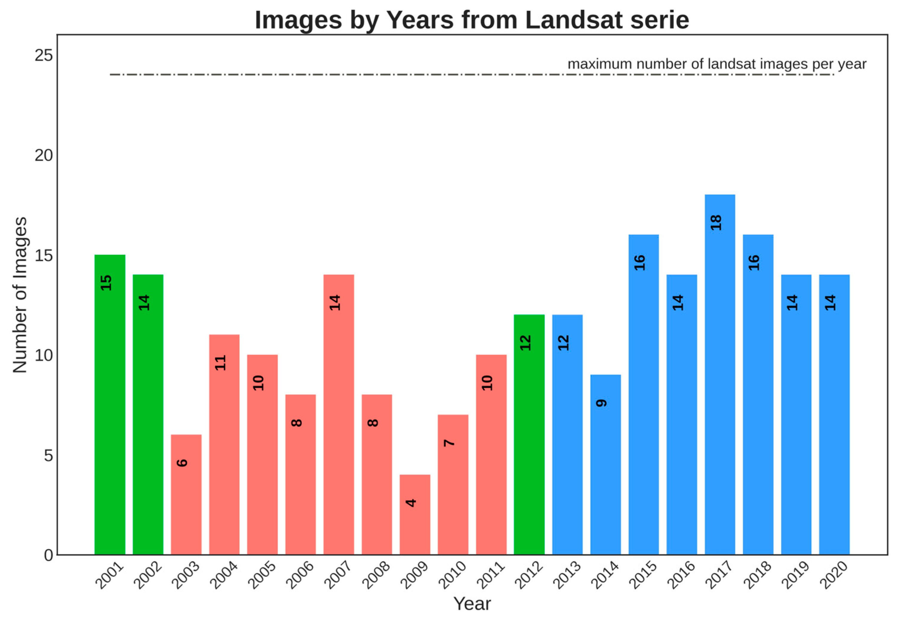
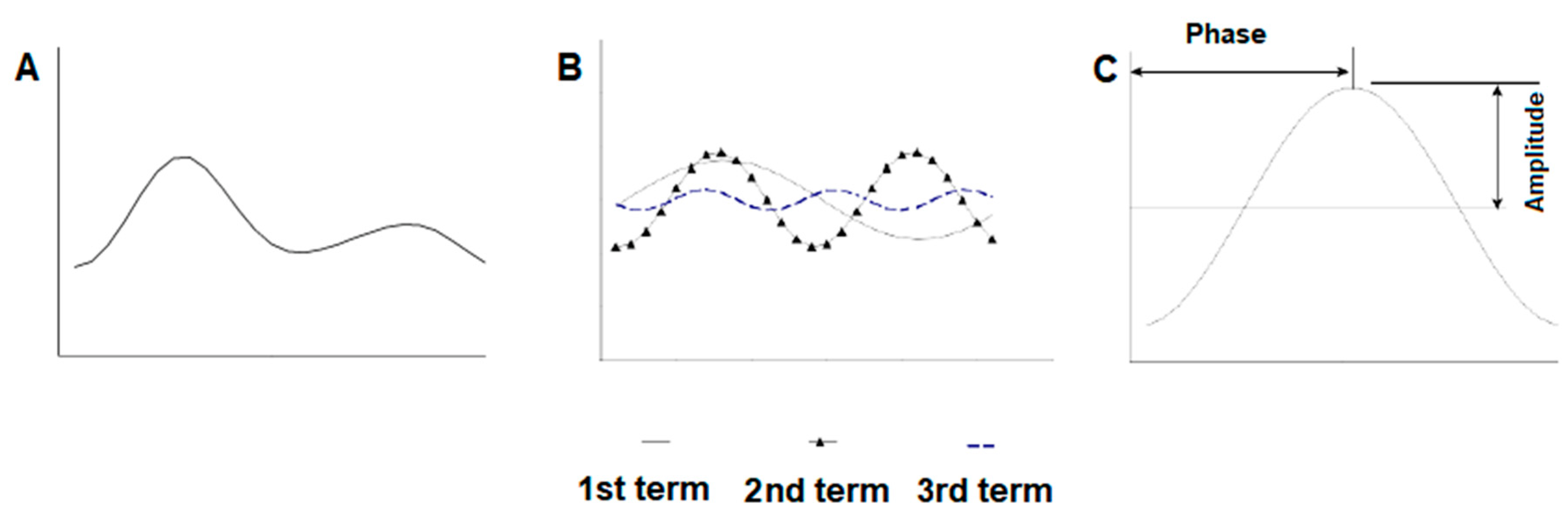
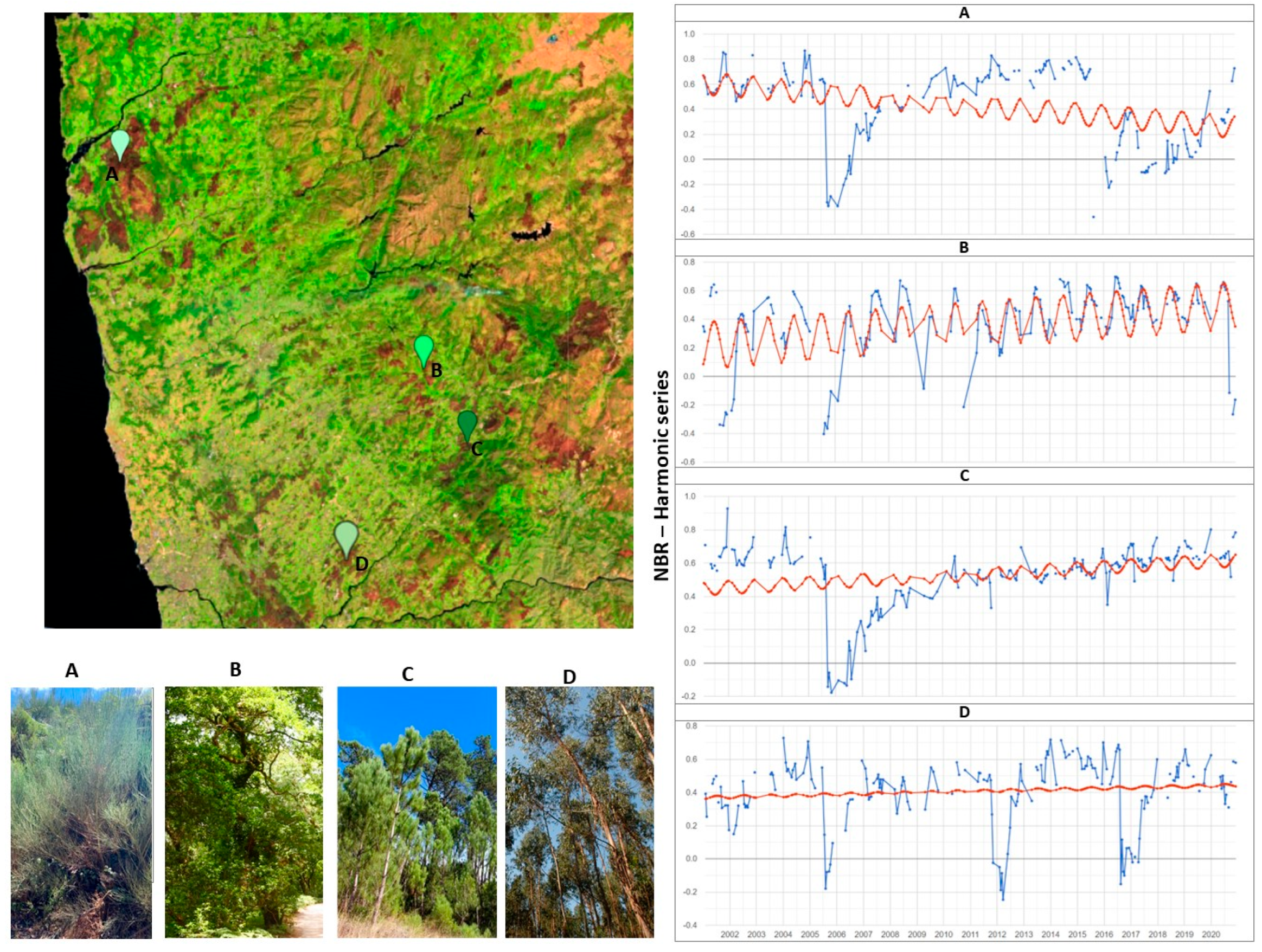
Data Analysis and Exploration of Landsat Time Series Data from 2001 to 2020

In a first phase, sample points were collected for burnt and non-burnt areas, with consideration for the different sub-classes described previously. A total of 80 points were collected for the burnt class and 107 points for the non-burnt class. For this step, the corresponding NBR, MIRBI, BAI, and dNBR spectral indices for these points were analysed. From several controlled points in the series, the values of the indices and the breaks in trends in the fire dates within the series were inspected. The NBR was the index that best represented these series trend breaks, and based on the feature selection approach, it was defined as the index for the adjustment of the harmonic model in the time series.

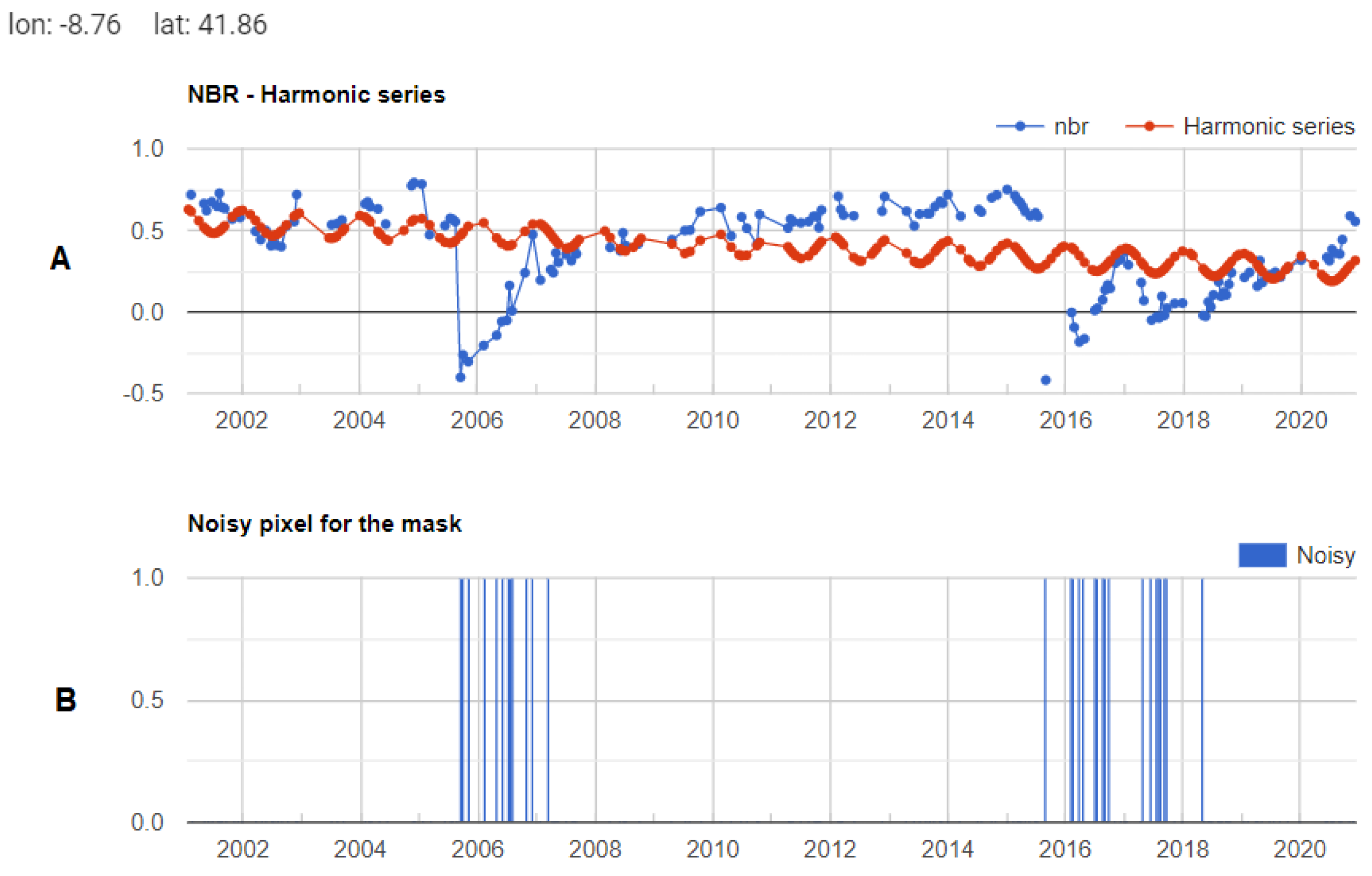
Outlier Detection in the Time Series

In burnt area detection results, the first step was to identify pixels with negative discrepant values in relation to the observed reflectance over time in the time series, which indicated the possible burnt areas, called outliers, and then to perform the classification. For this, we considered the difference in phenology in the study area and the data gathered to detect possible burnt areas. We used the Fourier harmonic model [72,73] to analyse the time series in remote sensing data [73,74,75,76,77,78].

The harmonic model allows a complex curve to be expressed as the sum of a series of cosine waves [72,73]. A time series of remote sensing data (Figure 4A) can be deconstructed using the Fourier series into a set of simple cosine waves of different frequencies (Figure 4B). Several frequency terms add up to form the original complex curve. Each cosine is defined by phase, which is equal to the displacement of the wave from the origin (Figure 4C); amplitude, which is equal to half the height of the wave (Figure 4C); and frequency, which is equal to the number of complete wave cycles in the unit time [72,73,78].

The method consisted of three steps. First, we generated image stacks of the NBR spectral index of the 16-day Landsat 5, 7, and 8 time series for the 20 years. Second, we adjusted the time series harmonic model using the observations of the NBR spectral index within the stable period as the dependent variable. The following model was fitted for each pixel (Equations (1) and (2)), where $y_t$ is a dependent variable (NBR), t is an independent variable (time as Julian date), $e_t$ is the residual error (random), A is the amplitude, $\omega$ is the frequency, and $\varnothing$ is the phase.

$$y_t={\beta }_0+{\beta }_{1}t+A\cos \left(2\pi \omega t-\varnothing \right)+e_t$$

(1)

We can decompose: Equation (1) to obtain Equation (2), that is, our function into separate cosine and sine elements:

$$y_t={\beta }_0+{\beta }_{1}t+{\beta }_2\cos \left(2\pi \omega t\right)+{\beta }_3\sin \left(2\pi \omega t\right)+e_t$$

(2)

where:

$${\beta }_2=A\cos (\varnothing ); {\beta }_3=A \sin (\varnothing ); A={({\beta }_2^2+{\beta }_3^2)}^{\raisebox{1ex}{$1$}\!\left/ \!\raisebox{-1ex}{$2$}\right.}; \mathrm{and} \varnothing =\mathrm{atan}({\beta }_3/{\beta }_2).$$

In the third step, we used a threshold to identify the possible burnt pixels, which were selected as outlier points between the harmonic series and the NBR data series. We calculated the values to compose the mask (M) by comparing the values observed in the actual and predicted data (Equation (3)). After identifying them, the mask of possible burnt areas was exported as an ImageCollection.

$$M=y_t-{\widehat{y}}_t$$

(3)

where $y_t$ and ${\widehat{y}}_t$ are the actual and expected observations, respectively.

2.2.3. Mask Classification Using Random Forests

Sample Collection

The areas to be classified were selected from the mask with the possible burnt areas. Each image in the series was classified within the mask, which reduced the analysis area of the classifier and possible spectral confusion between targets with similar signals (e.g.,: burnt area, relief shade and clouds, exposed soil, water, urban area).

Sample collections for classification were performed on 7 Landsat images: 2 Landsat 5, 2 Landsat 7, and 3 Landsat 8 (

Table 3. Description of the images used to collect the classification samples.

Sensor	Years	Rois
Landsat TM 7	2001, 2002 e 2012	[‘LE07_204031_20010915_normal_rois’, ‘LE07_204031_20021004_normal_rois’],
Landsat TM 5	2004, 2005, 2006, 2007, 2008, 2009, 2010 e 2011	[‘LT05_204031_20051004_normal_rois’, ‘LT05_204031_20101018_normal_rois’]
Landsat OLI 8	2013, 2014, 2015, 2016, 2017, 2018, 2019 e 2020	[‘LC08_204031_20131010_normal_rois’, ‘LC08_204031_20160916_normal_rois’, ‘LC08_204031_20170903_normal_rois’]

). The collections only considered the outlier values; therefore, these pixels labelled burnt and unburnt served for the model training.

Classification

Image classification was performed using the random forest classifier on GEE and was originally developed by Breiman et al. [46]. Random forest is a supervised classification algorithm that uses the ensemble methodology for classification. Ensemble methods group a finite set of classifiers, and the final decision of the class is made by either the majority vote of these classifiers or the maximum probability among them. These methods present better results in the literature. In the case of random forest, all classifiers are decision trees that are built by selecting both sets with fixed sizes of input variables at random and sample sets to build the trees.

For this work, the selection of the random forest classifier was made by two criteria: one was robustness, and the other was to be implemented in the work environment [46]. This classifier reduces the overfitting problem by randomly selecting both samples and variables to build each tree. It increases the accuracy by taking the various outputs of the different decision trees to the maximum vote criterion.

One of the most recent techniques used in machine learning is “Model Tuning”, which is nothing more than adjusting the hyperparameters of the model to improve the accuracy of the results and decrease the computational costs. To do it, we used the feature importance method to select the set of variables that best behaved in relation to the set of samples, wherein we used the library within the Google colab “scikit-learn y” of python as a database and as the training sample set.

The chosen method was the importance permutation of the variables or features that each tree within random forest assigned in the score method, which caused each tree in the model to assign a score to each variable during the training set, so after training the “feature_importances_” function of the model, a score was developed with values between 0 and 1, which allowed a list order, so the selection of variables was done based on a threshold to select the most important ones from an M number of the most important ones. We selected 14 variables out of 23 (

Table 4. Variables used to train the model, based on the order of importance for each sensor.

Sensor	Training Variable
L5	‘nir’, ’green’, ‘mirbi’, ‘swir1’, ‘blue’, ‘dnirr’, ‘nbr’, ‘dndvi’, ‘dmirbi’, ‘evi’, ‘dnbr’, ‘gndvi’, ‘ndmi’, ‘savi’
L7	‘nir’, ‘mirbi’, ‘red’, ‘evi’, ‘green’, ‘nbr’, ‘swir1’, ‘dnirr’, ‘dndvi’, ‘dnbr’, ‘ndmi’, ‘dmirbi’, ‘gndvi’, ‘blue’, ‘savi’
L8	‘nir’, ‘mirbi’, ‘dmirbi’, ‘evi’, ‘nbr’, ‘dnbr’, ‘green’, ‘dnirr’, ‘red’, ‘swir1’, ‘ndmi’, ‘gndvi’, ‘blue’, ‘savi’

).

In the model tuning step, several sets of model input parameters were tested, and those with best results for the random forest classifier were: RandomForestClassifier (n_estimators = 160, max_features = 6, min_samples_split = 10, oob_score = True, bootstrap = True).

This step allowed for the implementation of the classifier within the GEE platform; the hyperparameters that were already adjusted were used to classify each of the images from the historical series. The test set was built from the selection of several random images from the series using two conditions: each Landsat sensor must have at least two sample images, and the selected image must have several burnt area spots. Then, polygons were drawn in several parts of the image in a distributed way, for both burnt and unburnt areas, with the presence of covers that could lead to confusion in the classification mentioned above. Within these polygons, points were drawn, and the true points were drawn within the area of intersection with the ICNF government polygons. After that, these points were used to build the confusion matrix and calculate the appropriate metrics.

2.2.4. Post-Classification

A series of spatial and temporal filters were applied to the resulting classification. The spatial filter was used to remove burnt areas smaller than 100 ha. To obtain the information of the month in which the fire scar was mapped for the first time, a post-classification processing was performed to retrieve the date information of the pixel that was burnt, starting from the date present in the metadata of each classified image within the time series. Subsequently, the classification was vectorized and exported. The annual burnt area maps were the composition of all the burnt areas of each image in the respective year.

Reference Data

The reference data used in this research correspond to the Burnt Area product (in hectares) of the ICNF, which was elaborated following several stages, of which we highlighted the action of the National Republican Guard (GNR) and the involvement of municipal councils in: (i) the collection, survey, and production of geographic information, with the consequent creation of the polygon; (ii) the association of the survey to an occurrence with the attribution of the correct name to the generated file (KML); (iii) the loading of the polygons and associated information in the Forest Fire Information Management System application; (iv) the elaboration of the national cartography of burnt areas by compiling all KML files loaded in SGIF at the occurrence level and the correction of information faults with burnt area polygons from the semi-automatic classification processes using LANDSAT, SENTINEL, or other satellite images [79].

Assessment of Results

The measures that estimate how much accuracy a map has or the results of an output of machine learning algorithms are based on the error matrix (

Table 5. Matrix of error or contingency adapted from [81].

		Reference
	$P_{11}$	$P_{12}$	$P_{1.}$ = $P_{11}$+$P_{12}$
Classification	$P_{21}$	$P_{22}$	$P_{2.}$
	$P_{.1}$ = $P_{11}$+$P_{21}$	$P_{.2}$

) that calculates the pixels that were classified well, the pixels that erroneously went to the reference class and should have been in the class of the classification, and the pixels that were in the classification and should have been in the reference class [80]. The metrics of overall accuracy (Ac), the producer’s accuracy, and the user’s accuracy follow the equation Formulas (4)–(6) [80]:

$$Ac=P_{11}+P_{22}$$

(4)

$$producer’s accuracy=P_{11}/P_{.1}$$

(5)

$$user’s accuracy=P_{11}/P_{1.}$$

(6)

Recently used metrics include the quantity and allocation disagreement, which characterize disagreements between classes as an index [80,81]. The equation for quantity disagreement is calculated as follows:

$$Q=\left(\left|P_{.1}-P_{1.}\right|+\left|P_{2.}-P_{2.}\right|\right)/2$$

(7)

The quantity disagreement describes the number of pixels that are wrongly classified into the burnt area or unburnt area class.

The allocation disagreement or interchange difference is calculated as follows:

$$A=2\ast Minimum \left(P_{21},P_{12}\right)$$

(8)

The allocation disagreement or interchange quantifies the number of pixels that are correctly positioned on the map, but whose class value is modified. Therefore, this type of error normally has the same amount in the burnt class as in the unburnt class [81]. We also calculated the index values of precision, recall, F1-score, and IoU for the performance evaluation of the results [82].

The time series evaluation analysis of the burnt area was carried out based on ~158.000 randomly selected independent samples for the years 2001, 2002, 2005, 2010, 2013, and 2016 [83], which were chosen to ensure a representation of a greater and lesser extent of burnt area, and 2 years were selected by Landsat sensor. The images selected within these years had two criteria: low percentage of clouds and a high number of fires.

To select the areas to place the reference points of non-burnt areas, the images were visualized without any auxiliary mask, and scattered small polygons were created around the image while taking care not to include the burnt areas. These polygons were used to collect points randomly, with the polygon value used as a reference for the unburnt area and the RF classification value after the result.

Concerning the collection of the burnt area points, all images classified by year were combined, and points were raffled in polygons larger than 10 hectares from the ICNF mapping while taking the polygon value as a reference and the annual classification value as a class. All accuracy metrics, as well as commission and omission errors, were calculated on this basis of collected points as well.

3. Results

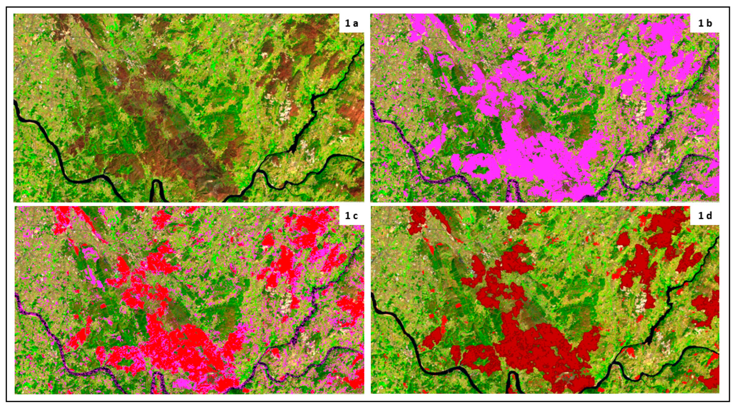
3.1. Mask with Outliers of Possible Burnt Areas

Figure 5 and Figure 6 illustrate how the outliers in the time series were identified from the application of the Fourier harmonic model to analyse the time series using the observations of the NBR spectral index [72,73,74,75,76,77,78]. The fire events resulted in a sudden and persistent decrease in the NBR, that is, a drop in its values observed in the series.

Fourier harmonic analysis provided estimates with the actual observed values of the NBR, which made it possible to compare and identify the threshold to select the pixels considered as outliers, or possible burnt areas, between the harmonic series and the real data series of the NBR [40,74]. Thus, values between +1.0 and −0.2 were eliminated from the time series, and those between −0.2 and −1.0 were considered outliers to generate the mask of possible burnt areas. Figure 6 shows an example of how the values were selected from the definition of the threshold.

3.2. Classification

Mapping wildfires using satellite data is a challenge, especially when performed in a study area with different types of land use and landscape characteristics [84]. Initially, the image collection consisted of 232 Landsat images. After the harmonic adjustment, the identification of outliers, and the definition of the mask, it totalled 172 images. Sixty of them that did not have pixels with values considered outliers were eliminated. The pixels classified by random forest were only those that were covered by the masked area, which contributed to the image processing, since not all pixels were considered for the classification process. Thus, the classifier was trained only with those that were possible burnt areas extracted from the first time series analysis. Hence, the set of pixels to be separated between the burnt area and not by the classifier was reduced spectrally to a smaller universe.

Figure 7 shows an example of a burnt area classification sequence for September 2005, in which we can observe the Landsat image with an example of the mask (Figure 7(1b)), and the final classification (Figure 7(1d)). This shows that burnt areas were generally well-delineated, especially in large fires.

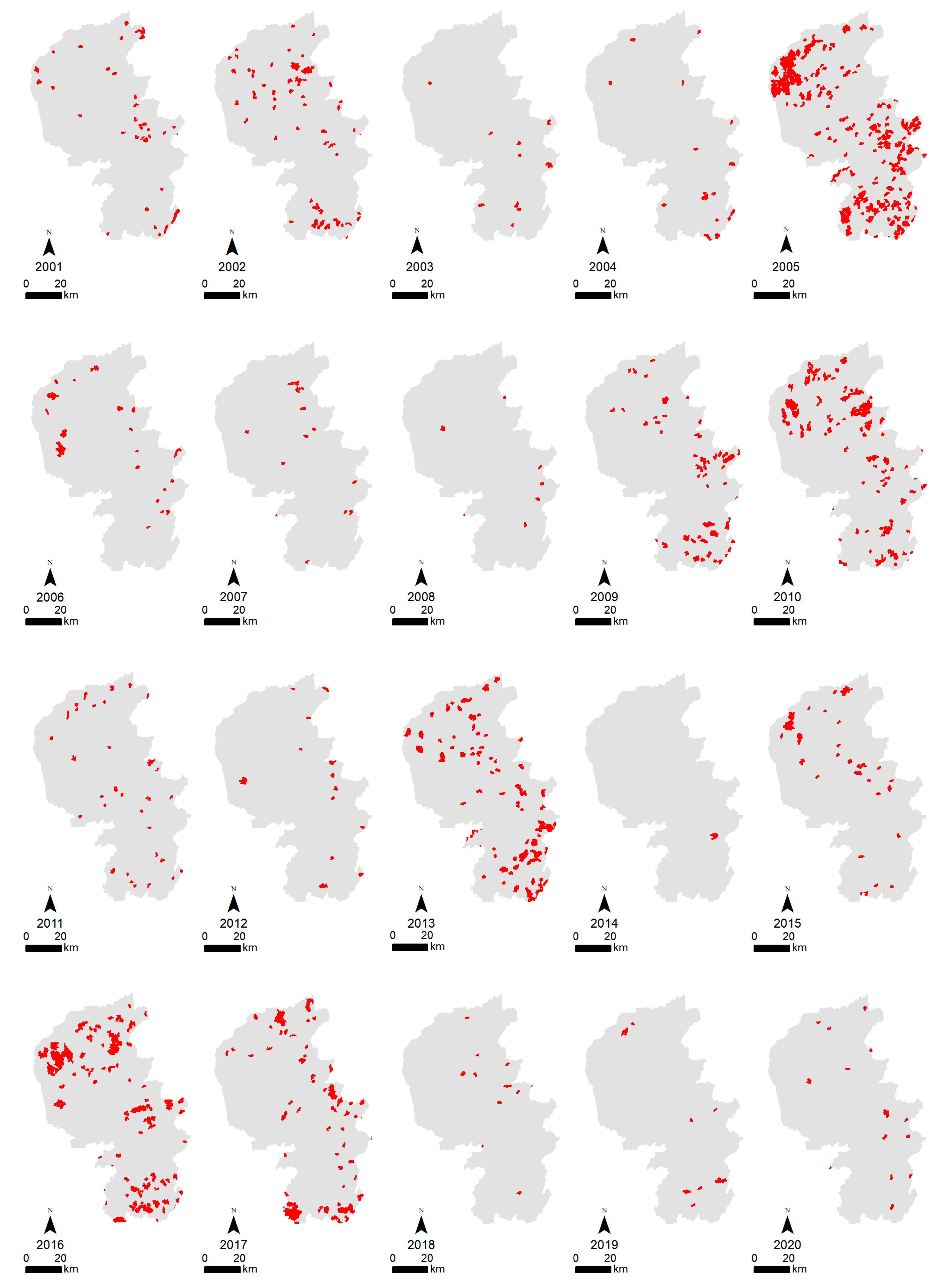
3.3. Annual Burnt Area

A burnt area dataset, based on the Landsat time series resulting from the classification, was created for northwestern Portugal. The burnt area maps revealed that ~23.5% of the territory was burnt at least once from 2001 to 2020 (Figure 8). The temporal variability of the burnt area indicated that, on average, 6.504 hectares were affected by large fires within the 20 years. The annual burnt area varied over the years, with the minimum annual area detected in 2014 (679.5 hectares) and the maximum mapped area detected in 2005 (73,025.1 hectares).

The other years in which the occurrence of large fires peaked (above 10,000 hectares) were 2002, 2009, 2010, 2013, 2016, and 2017, while those with the smallest burnt area (less than 2000 ha) included the years 2003, 2007, 2012, 2014, and 2018. Most of these years suffered from climate anomalies, which promoted extreme droughts, which were influenced by El Niño or an increase in precipitation (La Niña) [28,84].

We can see that in the 20 years analysed, there was a reduction in the burnt area from 2006 to 2015 compared to the period from 2001 to 2005, followed by an increase when compared with 2016 to 2020 (

Table 6. Number and burnt area of LW (≥100 ha) in Portugal mainland.

Years	N° of Polygons	Burnt Area (ha)
2001–2005	271	99.03844
2006–2010	184	54.77502
2011–2015	47	48.01547
2016–2020	185	75.72701

).

When dealing with studies on large fires, it is important to understand the different dimensions of occurrences. By analysing the size of the fires identified in the classification, we could note that the large wildfires (>100–500 ha) represented 43% of the burnt area, and they reached 100% of occurrences in the years 2003, 2004, 2007, 2008, and 2018 (Figure 9 and Figure 10). A total of 25.3% of the total burnt area concerned occurrences between 500 and 1000 ha, and in 2014, 100% of the area was included in this category. A total of 26% of the burnt area was between 1000 and 10,000 hectares in size; we observed that the years 2016 and 2017 were the only ones that presented an area greater than 45% for this category. Only 6% of the area corresponded to fires greater than 10,000 hectares, which occurred in Viana do Castelo in 2015 (Figure 11).

The reality of large fires in Portugal has gone through different stages in terms of its extent. In the 1970s, the LW became quite common, but it was only after the 1980s that they reached areas greater than 10,000 ha [85]. During the 1990s, there was an increase in records, and, from the 2000s onwards, records of an area of more than 20,000 ha were verified, which showed that there was an increase in the individual area of the largest LW in terms of the space and the incidence [27,86].

3.4. Results Evaluation

With the base of points for validation, we calculated all the metrics below. This set had three pieces of information per point: class, reference, and year. Thus, it was possible to evaluate both by year and by series using all the points. The burnt area of the Landsat time series achieved an overall accuracy of 92.1% (Figure 12).

The validation results for our time series burnt area classification approach are shown in

Table 7. Validation results for all years.

	Unburnt (Reference)	Burnt (Reference)	User’s Total	User’s Accuracy
Unburnt	56,358	2359	58,717	95.98%
Burnt	14,208	85,159	99,367	85.7%
Producer’s total	70,566	87,518	158,084
Producer’s accuracy	79.87%	97.3%

. They demonstrate satisfactory results for the burnt area classification, with a producer’s accuracy of 97.3% for the burnt area class in all years (with a minimum of 94.5% for 2010 and a maximum of 99.92% for 2001). The user’s accuracy reached a value of 85.7% for the burnt area class for all years (minimum of 76.94% for 2010 and 91.81% for 2002). These accuracy values for the producer and user indicate that the method has few commission and omission errors. For the unburnt class, the producer’s accuracy was 79.87% for all years, and the user’s accuracy was 95.98%. In the last ones, it was estimated that the algorithm contained more commission errors than omission errors and was good for the burnt area detection process.

Another very interesting analysis is to understand the behaviour of errors in the classification analysis. We calculated the metrics of quantity disagreement and allocation disagreement [81,87]. Figure 13 inverts the values of the metrics to make it easier to understand that there were signalling errors.

In this analysis, we had a high percentage of allocation disagreement or interchange in the year 2010, which indicated that 12.14% of the pixels used for the analysis in that year were in the correct position but had changed classes. In that same year, the quantity disagreement indicated 6.2% of the pixels, which made us understand that this percentage of pixels, in addition to being erroneously classified as fire, were also misallocated.

Figure 14 presents the result validation metrics of recall, precision, F1-score, and IoU. In general, all years presented precisions above 0.9. Recall values closer to 1 mean that there is a higher probability of success, and all years presented recall values of more than 0.8, except for 2010, when it was around 0.7. For F1-score and IoU indices, the year 2010 also presented the least satisfactory results.

4. Discussion

In this work, we developed a methodology to map large wildfires in northwestern Portugal using a ML algorithm and time series of Landsat images, which can be expanded to other areas. For the classification of burnt areas, the authors initially used the Fourier harmonic model to define outliers in the time series representing pixels of possible burnt areas and then applied the random forest classifier for LW classification.

Approaches based on remote sensing play a key role in vegetation monitoring, as they provide a better opportunity to map changes and identify fire [76]. Satellite data have significant potential for monitoring vegetation dynamics from regional to global scales, due to synoptic coverage and regular temporal sampling [75]. The NBR was chosen because it is an appropriate index to detect changes in the landscape induced by fires, and it evaluates them in the spectral response caused by burnt areas [88].

In satellite remote sensing observation, vegetation greenness patterns follow a trend, with peak greenness at the height of the growing season in late spring, decreased greenness when vegetation senesces during the summer, and, frequently, a secondary muted peak or plateau in greenness, especially in some cool seasons. Thus, the calculation of vegetation indices lowers the value (NBR) immediately after fire [78].

The construction of a harmonic model is used in remote sensing applications, due to its flexibility in accounting for cyclicity in simple and reproducible ways. If there is a seasonal trend in the data, the ordered nature of a cosine curve can probably approximate it [89].

In regions such as northwestern Portugal, which registers high values of precipitation and cloud cover during the year, the low availability of observations (images) in certain years makes the pixel time series irregular and can pose a challenge for that type of analysis; however, our method was still able to capture changes in vegetation. A similar fact occurred in a study developed by DeVries et al. [76], who captured a sign of change in the forest (deforestation) by applying methodology using Fourier analysis and the time series.

The mask served to avoid confusion between burnt areas and other land cover dynamics, which were verified in the previous stage of data analysis (for instance, urban area, exposed soil). The application of harmonic analysis produced computationally efficient quantitative time estimates of post-fire vegetation patterns that were considered within the time series, as was seen in a study undertaken in a pasture area to estimate the variability of time between fires and vegetation regrowth [78].

The use of the mask showed great potential in the development of this study, as it reduced the number of pixels to be classified by keeping only pixels with spectral behaviour with characteristics of an area that has suffered from the action of fire. In this way, the universe of pixels to be classified only included a reduced set of pixels in the image, where the difference to be found to separate this set into two classes was more specific to the group than to the set of pixels in the whole image.

The combination of the Landsat time series and harmonic model adjustment proved to be an effective method for the annual detection of burnt areas in the study area, mainly in forest and wild spaces. It has also been demonstrated by other studies that temporal information and the harmonic model can be successfully applied to detect land cover changes based on the Landsat time series [40,74,90].

Concerning the classification, the ephemeral characteristics of the fire scars left on satellite images are a complicating factor for the detection of burnt areas. Depending on the frequency of observation and the fire intensity, it is possible to lose the spectral signature of the fire in the landscape [84,91]. Moreover, seasonality plays a central role in the temporal change of the spectral information of a fire scar by creating artificial signals that confuse the dry signals of the SWIR 1 and SWIR 2 channels in the arid areas during the dry season with the spectral responses of the ash, which also show lower reflectance signals in water-sensitive channels [84,92].

We can highlight examples of classifier confusion in areas with bush vegetation and in agricultural land. In the area with bush type vegetation, mainly in the mountainous regions to the northeast of the study area, the spectral signature of the burnt area disappears in a few weeks, which can be influenced by the amount of available vegetation and the influence of the reflectance of the exposed rock in that region. On the other hand, agricultural land that during some months of the year are without vegetation, that is, bare soils, present a spectral signal very similar to the spectral information of a fire scar.

In the case of the Mediterranean forest, fire patches can be easily confused with agricultural burns or even with bare soils, which often reach saturation temperature in the summer during late afternoon [93]. The spatial and temporal variability of the spectral signatures of burnt areas shows diverse and complex patterns, and, despite the large number of different classifiers used to detect and map them, it remains somewhat problematic to discriminate scar signals from those of other land cover types. The types of surfaces most reported to generate spectral confusion with burnt areas are water surfaces, urban areas, and shadows [93], which were observed in the results of this study.

Thus, we can relate that the years with the greatest availability of images without cloud cover, between March to December, which are the main months that registered the major fires in the study area, have a greater potential for mapping them with the proposed methodology. In this context, Portugal is the European country with the highest percentage of the territory affected by wildfires impacting its forest cover, which mainly consists of plantations of shrubland, including Pinus pinaster and Eucalyptus globulus, that burn more easily than the native Quercus faginea and Quercus suber [94]. In the country, fires are evenly distributed throughout the territory, and the northwest has the highest incidence of wildfires [95].

Hence, the occurrence of major fires in Portugal is not unknown [55,56]. Authors, such as Ferreira-Leite et al. [86], argue that large fires are not a recent phenomenon in the country, as they have been a common reality since at least the 19th century. What has changed is the frequency and size of affected areas [27,86].

The occurrence of extreme weather events (e.g., heat waves) and climate variability (e.g., drought), which also tend to be more frequent and intense during the summer, are the main contributors to this pronounced seasonal character of wildfire incidence in Portugal [14,24,96,97].

The northern region is characterized not only by a much higher density of fire numbers and burnt area compared to the rest of the country [20,24,98], but also by more irregular topography, a denser river network, a higher concentration of forest, and population density, as well as a colder and rainier climate [20,99,100]. Therefore, it is important to consider that the spatial distribution of ignitions and the burnt area are also highly dependent on other human and biophysical aspects, such as demographic, socioeconomic, topographic, land use, and land cover factors [24,101].

In terms of accuracy, the error is in the commission. This is an algorithm that omits little fire, but still confuses some unburnt areas with the burnt area. Some factors possibly influenced the results, such as (i) data gaps in the time series due to the high fraction of cloud coverage and cloud shadow [29]; (ii) similar spectral behaviour between areas affected by fires with the spectral behaviour of bare soil, rocks, water, and relief shadows; and (iii) the reference data having been produced using different data and with field information. Related studies conducted in Africa found a similar accuracy of 79.2% [74]. The year with the highest accuracy was 2002, despite not being the one with the highest number of burnt areas, nor the one with the largest patches.

This allocation disagreement indicates that the same number of pixels that were counted as commission, because they were classified as fire and not in the reference, were also counted in omission, because they were points that were extracted from the reference polygons. The quantity disagreement was the more critical type of error than the previous one, because if all pixels with allocation errors changed classes, they would be corrected, and the class of the year 2005, for example, would have better accuracy than 2016, so 2010 was the year with the worst performance within the series.

There are other ways to validate the results, such as using calculated recall, precision, F1-score, and IoU. Precision is more focused on the estimated class and, in this case, the burnt area class. Therefore, it measures the probability of the correct detection of fire values against all fire reference pixels. In this way, the index returns a probability of how much our classification was right, and the closer to 1 it is, the less omitted it is. As the graph reports in all years, the accuracy was good.

Recall is also an index focused on the estimated class, and it is the ratio of all correctly classified fire class pixels among all the classified pixels as fire. So, the closer to 1 it is, the higher the probability of correctness. In the graph (Figure 14), the recall values in all years were lower than the precision index, which means that the classifier found more false negatives, that is, the commission.

The F1-score and the IoU indices are also focused on the estimated class, and they encompass the correctly classified pixels with the misclassified ones. As the graph shows (Figure 14), the F1-score is higher than the IoU because in the calculation, it assigned a greater value to the correctly classified pixels; thus, in the literature, the F1-score is more frequently used than the IoU.

5. Conclusions

We explored the potential of using the Landsat time series to develop a methodology that would allow for the annual mapping of large wildfires. This methodology used a machine learning algorithm based on a harmonic model and the identification of outliers. The algorithm used 172 Landsat images between January 2001 and December 2020, and the results were compared with the burnt area data produced by the Portuguese government.

We concluded that the process of defining the mask with the outliers considerably reduced the universe of pixels to be classified within each image, which left the training of the classifier focused on separating the set of pixels into two groups with very similar spectral characteristics, which contributed so that the separation of groups with similar spectral behaviour was performed automatically and without great sampling effort.

The use of spectral indices and some specific bands broadened the spectral space characterization, which allowed a better selection in the feature selection analysis steps. The analysis of the feature selection using an indicator that made it possible to choose the best bands for the classifier to provide a more compact feature space with better performance, thereby expecting a better result in the classification step. The analysis of the classification parameters made the classification step use those parameters, which led to a better performance of the algorithm with this data and in this problem.

Although we only used the Landsat series data, we achieved satisfactory results when considering that the reference data (ICNF) are generated from multiple sensors. The method showed satisfactory accuracy results with little omission for burnt areas. With the results of the classification, we were able to identify unburnt areas within the LW perimeters, which represents an important factor for research on this issue when considering that the identification of these unburnt areas can contribute to the understanding of the dynamics related to different intensities and severities reached by LW, which can make advances in studies in this field. One of the ways to improve the classification results would be the application of deep learning methods, which can be a means of having an algorithm with less commission. This methodology can be used for any remote sensing problem that leads to the detection of some disturbance along the time series. We recommend that this analysis has at least five years of data to obtain meaningful results. Therefore, we can indicate the use of this method for studies in other similar areas, such as deforestation and drought events, for example.

References

1. Bar, S.; Parida, B.R.; Pandey, A.C. Landsat-8 and Sentinel-2 based Forest fire burn area mapping using machine learning algorithms on GEE cloud platform over Uttarakhand, Western Himalaya. Remote Sens. Appl. Soc. Environ. 2020, 18, 100324. [Google Scholar] [CrossRef]
2. Langmann, B.; Duncan, B.; Textor, C.; Trentmann, J.; van der Werf, G.R. Vegetation fire emissions and their impact on air pollution and climate. Atmos. Environ. 2009, 43, 107–116. [Google Scholar] [CrossRef]
3. Kalantar, B.; Ueda, N.; Idrees, M.O.; Janizadeh, S.; Ahmadi, K.; Shabani, F. Forest Fire Susceptibility Prediction Based on Machine Learning Models with Resampling Algorithms on Remote Sensing Data. Remote Sens. 2020, 12, 3682. [Google Scholar] [CrossRef]
4. Kalivas, D.P.; Petropoulos, G.P.; Athanasiou, I.M.; Kollias, V.J. An intercomparison of burnt area estimates derived from key operational products: The Greek wildland fires of 2005–2007. Nonlinear Process. Geophys. 2013, 20, 397–409. [Google Scholar] [CrossRef] [Green Version]
5. Colson, D.; Petropoulos, G.P.; Ferentinos, K.P. Exploring the Potential of Sentinels-1 & 2 of the Copernicus Mission in Support of Rapid and Cost-effective Wildfire Assessment. Int. J. Appl. Earth Obs. Geoinf. 2018, 73, 262–276. [Google Scholar] [CrossRef]
6. Brown, A.R.; Petropoulos, G.P.; Ferentinos, K.P. Appraisal of the Sentinel-1 & 2 use in a large-scale wildfire assessment: A case study from Portugal’s fires of 2017. Appl. Geogr. 2018, 100, 78–89. [Google Scholar] [CrossRef]
7. Dos Santos, S.M.B.; Bento-Gonçalves, A.; Vieira, A. Research on Wildfires and Remote Sensing in the Last Three Decades: A Bibliometric Analysis. Forests 2021, 12, 604. [Google Scholar] [CrossRef]
8. Dos Santos, S.M.B.; Bento-Gonçalves, A.; Franca-Rocha, W.; Baptista, G. Assessment of Burned Forest Area Severity and Postfire Regrowth in Chapada Diamantina National Park (Bahia, Brazil) Using dNBR and RdNBR Spectral Indices. Geosciences 2020, 10, 106. [Google Scholar] [CrossRef] [Green Version]
9. Pausas, J.G.; Keeley, J.E. A Burning Story: The Role of Fire in the History of Life. Bioscience 2009, 59, 593–601. [Google Scholar] [CrossRef] [Green Version]
10. Pausas, J.G.; Keeley, J.E. Wildfires and global change. Front. Ecol. Environ. 2021, 19, 387–395. [Google Scholar] [CrossRef]
11. Bento-Gonçalves, A.; Vieira, A.; Úbeda, X.; Martin, D. Fire and soils: Key concepts and recent advances. Geoderma 2012, 191, 3–13. [Google Scholar] [CrossRef]
12. Mohajane, M.; Costache, R.; Karimi, F.; Bao Pham, Q.; Essahlaoui, A.; Nguyen, H.; Laneve, G.; Oudija, F. Application of remote sensing and machine learning algorithms for forest fire mapping in a Mediterranean area. Ecol. Indic. 2021, 129, 107869. [Google Scholar] [CrossRef]
13. Pereira, M.; Calado, T.; DaCamara, C.; Calheiros, T. Effects of regional climate change on rural fires in Portugal. Clim. Res. 2013, 57, 187–200. [Google Scholar] [CrossRef] [Green Version]
14. Pereira, M.G.; Aranha, J.; Amraoui, M. Land cover fire proneness in Europe. For. Syst. 2014, 23, 598. [Google Scholar] [CrossRef]
15. Fernandes, P.M. Fire-smart management of forest landscapes in the Mediterranean basin under global change. Landsc. Urban Plan. 2013, 110, 175–182. [Google Scholar] [CrossRef] [Green Version]
16. Tedim, F.; Leone, V.; Amraoui, M.; Bouillon, C.; Coughlan, M.; Delogu, G.; Fernandes, P.; Ferreira, C.; McCaffrey, S.; McGee, T.; et al. Defining Extreme Wildfire Events: Difficulties, Challenges, and Impacts. Fire 2018, 1, 9. [Google Scholar] [CrossRef] [Green Version]
17. Inbar, A.; Lado, M.; Sternberg, M.; Tenau, H.; Ben-Hur, M. Forest fire effects on soil chemical and physicochemical properties, infiltration, runoff, and erosion in a semiarid Mediterranean region. Geoderma 2014, 221, 131–138. [Google Scholar] [CrossRef]
18. Noss, R.F.; Franklin, J.F.; Baker, W.L.; Schoennagel, T.; Moyle, P.B. Managing fire-prone forests in the western United States. Front. Ecol. Environ. 2006, 4, 402–407. [Google Scholar] [CrossRef] [Green Version]
19. Nunes, A.N. Regional variability and driving forces behind forest fires in Portugal an overview of the last three decades (1980–2009). Appl. Geogr. 2012, 34, 576–586. [Google Scholar] [CrossRef]
20. Parente, J.; Pereira, M.G. Structural fire risk: The case of Portugal. Sci. Total Environ. 2016, 573, 883–893. [Google Scholar] [CrossRef]
21. Hernández, L. Paisagens Corta-Fogos. Proposta da ANP|WWF e WWF Espanha Para um Território Ibérico Adaptado aos Incêndios. 2021. Available online: https://wwfeu.awsassets.panda.org/downloads/final_wwf_informeincendios_2021_pt_af_low.pdf (accessed on 11 September 2022).
22. Vilar, L.; Camia, A.; San-Miguel-Ayanz, J.; Martín, M.P. Modeling temporal changes in human-caused wildfires in Mediterranean Europe based on Land Use-Land Cover interfaces. For. Ecol. Manage. 2016, 378, 68–78. [Google Scholar] [CrossRef]
23. Kanevski, M.; Pereira, M.G. Local fractality: The case of forest fires in Portugal. Phys. A Stat. Mech. Its Appl. 2017, 479, 400–410. [Google Scholar] [CrossRef] [Green Version]
24. Parente, J.; Pereira, M.G.; Amraoui, M.; Tedim, F. Negligent and intentional fires in Portugal: Spatial distribution characterization. Sci. Total Environ. 2018, 624, 424–437. [Google Scholar] [CrossRef] [Green Version]
25. Bento-Gonçalves, A.; Vieira, A.; da Vinha, L. Safa’Hamada Changes in mainland Portuguese forest areas since the last decade of the XXth century Changements des zones forestières portugaises depuis la dernière décennie du xxe siècle. Méditerranée 2018, 130, 10025. [Google Scholar] [CrossRef]
26. Lourenço, L.; Bento-Gonçalves, A.; Vieira, A.; Nunes, A.; Ferreira-Leite, F. Forest Fires in Portugal. In Portugal: Economic, Political and Social Issues; Bento-Gonçalves, A., Vieira, A., Eds.; Nova Science Publishers: New York, NY, USA, 2012; pp. 97–112. ISBN 978-1-62257-523-7. [Google Scholar]
27. Ferreira-Leite, F.; Bento-Gonçalves, A.; Vieira, A.; Nunes, A.; Lourenço, L. Incidence and recurrence of large forest fires in mainland Portugal. Nat. Hazards 2016, 84, 1035–1053. [Google Scholar] [CrossRef]
28. Ferreira-Leite, F.; Ganho, N.; Bento-Gonçalves, A.; Botelho, F. Iberian atmosferic dynamics and large forest fires in mainland Portugal. Agric. For. Meteorol. 2017, 247, 551–559. [Google Scholar] [CrossRef]
29. Chuvieco, E.; Mouillot, F.; van der Werf, G.R.; San Miguel, J.; Tanasse, M.; Koutsias, N.; García, M.; Yebra, M.; Padilla, M.; Gitas, I.; et al. Historical background and current developments for mapping burned area from satellite Earth observation. Remote Sens. Environ. 2019, 225, 45–64. [Google Scholar] [CrossRef]
30. Koutsias, N.; Pleniou, M. A rule-based semi-automatic method to map burned areas in Mediterranean using Landsat images–revisited and improved. Int. J. Digit. Earth 2021, 11, 1602–1623. [Google Scholar] [CrossRef]
31. Goodwin, N.R.; Collett, L.J. Development of an automated method for mapping fire history captured in Landsat TM and ETM + time series across Queensland, Australia. Remote Sens. Environ. 2014, 148, 206–221. [Google Scholar] [CrossRef]
32. Ngadze, F.; Mpakairi, K.S.; Kavhu, B.; Ndaimani, H.; Maremba, M.S. Exploring the utility of Sentinel-2 MSI and Landsat 8 OLI in burned area mapping for a heterogenous savannah landscape. PLoS ONE 2020, 15, e0232962. [Google Scholar] [CrossRef]
33. Zhang, P.; Ban, Y.; Nascetti, A. Learning U-Net without forgetting for near real-time wildfire monitoring by the fusion of SAR and optical time series. Remote Sens. Environ. 2021, 261, 112467. [Google Scholar] [CrossRef]
34. Ban, Y.; Zhang, P.; Nascetti, A.; Bevington, A.R.; Wulder, M.A. Near Real-Time Wildfire Progression Monitoring with Sentinel-1 SAR Time Series and Deep Learning. Sci. Rep. 2020, 10, 1322. [Google Scholar] [CrossRef] [Green Version]
35. Filipponi, F. Exploitation of Sentinel-2 Time Series to Map Burned Areas at the National Level: A Case Study on the 2017 Italy Wildfires. Remote Sens. 2019, 11, 622. [Google Scholar] [CrossRef] [Green Version]
36. Bright, B.C.; Hudak, A.T.; Kennedy, R.E.; Braaten, J.D.; Henareh Khalyani, A. Examining post-fire vegetation recovery with Landsat time series analysis in three western North American forest types. Fire Ecol. 2019, 15, 8. [Google Scholar] [CrossRef] [Green Version]
37. Martin, P.; Gómez, I.; Chuvieco, E. Performance of a burned-area index ( BAIM ) for mapping Mediterranean burned scars from MODIS data. In Proceedings of the 5th International Workshop on Remote Sensing and GIS Applications to Forest Fire Management: Fire Effects Assessment, Zaragoza, Spain, 16–18 June 2005; pp. 193–197. [Google Scholar]
38. Tran, B.; Tanase, M.; Bennett, L.; Aponte, C. Evaluation of Spectral Indices for Assessing Fire Severity in Australian Temperate Forests. Remote Sens. 2018, 10, 1680. [Google Scholar] [CrossRef] [Green Version]
39. Van Dijk, D.; Shoaie, S.; van Leeuwen, T.; Veraverbeke, S. Spectral signature analysis of false positive burned area detection from agricultural harvests using Sentinel-2 data. Int. J. Appl. Earth Obs. Geoinf. 2021, 97, 102296. [Google Scholar] [CrossRef]
40. Liu, J.; Maeda, E.E.; Wang, D.; Heiskanen, J. Sensitivity of Spectral Indices on Burned Area Detection using Landsat Time Series in Savannas of Southern Burkina Faso. Remote Sens. 2021, 13, 2492. [Google Scholar] [CrossRef]
41. Mpakairi, K.S.; Ndaimani, H.; Kavhu, B. Exploring the utility of Sentinel-2 MSI derived spectral indices in mapping burned areas in different land-cover types. Sci. Afr. 2020, 10, e00565. [Google Scholar] [CrossRef]
42. Lary, D.J.; Alavi, A.H.; Gandomi, A.H.; Walker, A.L. Machine learning in geosciences and remote sensing. Geosci. Front. 2016, 7, 3–10. [Google Scholar] [CrossRef] [Green Version]
43. Lary, D.J. Artificial Intelligence in Geoscience and Remote Sensing. In Geoscience and Remote Sensing New Achievements; InTech: London, UK, 2010. [Google Scholar]
44. Zhao, F.; Feng, S.; Xie, F.; Zhu, S.; Zhang, S. Extraction of long time series wetland information based on Google Earth Engine and random forest algorithm for a plateau lake basin–A case study of Dianchi Lake, Yunnan Province, China. Ecol. Indic. 2023, 146, 109813. [Google Scholar] [CrossRef]
45. Nasiri, V.; Beloiu, M.; Asghar Darvishsefat, A.; Griess, V.C.; Maftei, C.; Waser, L.T. Mapping tree species composition in a Caspian temperate mixed forest based on spectral-temporal metrics and machine learning. Int. J. Appl. Earth Obs. Geoinf. 2023, 116, 103154. [Google Scholar] [CrossRef]
46. Breiman, L. Random Forests. Mach. Learn. 2001, 45, 5–32. [Google Scholar] [CrossRef] [Green Version]
47. Lasaponara, R.; Abate, N.; Fattore, C.; Aromando, A.; Cardettini, G.; Di Fonzo, M. On the Use of Sentinel-2 NDVI Time Series and Google Earth Engine to Detect Land-Use/Land-Cover Changes in Fire-Affected Areas. Remote Sens. 2022, 14, 4723. [Google Scholar] [CrossRef]
48. Piao, Y.; Lee, D.; Park, S.; Kim, H.G.; Jin, Y. Forest fire susceptibility assessment using google earth engine in Gangwon-do, Republic of Korea. Geomat. Nat. Hazards Risk 2022, 13, 432–450. [Google Scholar] [CrossRef]
49. Pontes-Lopes, A.; Dalagnol, R.; Dutra, A.C.; de Jesus Silva, C.V.; de Alencastro Graça, P.M.L.; de Oliveira e Cruz de Aragão, L.E. Quantifying Post-Fire Changes in the Aboveground Biomass of an Amazonian Forest Based on Field and Remote Sensing Data. Remote Sens. 2022, 14, 1545. [Google Scholar] [CrossRef]
50. Tavakkoli Piralilou, S.; Einali, G.; Ghorbanzadeh, O.; Nachappa, T.G.; Gholamnia, K.; Blaschke, T.; Ghamisi, P. A Google Earth Engine Approach for Wildfire Susceptibility Prediction Fusion with Remote Sensing Data of Different Spatial Resolutions. Remote Sens. 2022, 14, 672. [Google Scholar] [CrossRef]
51. Jain, P.; Coogan, S.C.P.; Subramanian, S.G.; Crowley, M.; Taylor, S.; Flannigan, M.D. A review of machine learning applications in wildfire science and management. Environ. Rev. 2020, 28, 478–505. [Google Scholar] [CrossRef]
52. Vieira, A.; Bento-Gonçalves, A. Riscos Geomorfológicos no Noroeste de Portugal. Livro Guia da Visita Técnica No. 3; RISCOS: Coimbra, Portugal, 2020; ISBN 9789895494231. [Google Scholar]
53. Bento-Gonçalves, A.; Vieira, A.; Costa, F.; Lourenço, L.; Ferreira-Leite, F.; Marçal, V. Manifestações de Riscos no Noroeste de Portugal-Livro-Guia da Viagem de Estudo do III Congresso Internacional de Riscos; RISCOS: Coimbra, Portugal, 2014. [Google Scholar]
54. Vieira, A.; Bento-Gonçalves, A.; Ferreira-Leite, F. Geographic characterization. In Field trip Guidebook. 3rd International Meeting of Fire Effects on Soil Properties; Bento-Gonçalves, A., Vieira, A., Eds.; CEGOT, Universidade do Minho: Guimarães, Portugal, 2011; pp. 11–16. ISBN 978-989-97214-1-8. [Google Scholar]
55. Fernandes, S.; Lourenço, L. Grandes incêndios florestais de março, junho e outubro (fora do período crítico) em Portugal continental. Territorium 2018, 26, 15–34. [Google Scholar] [CrossRef]
56. Ferreira-leite, F.; Bento-Gonçalves, A.; Lourenço, L. Grandes incêndios florestais em Portugal continental. Da história recente à atualidade. Cad. Geogr. 2012, 30, 81–86. [Google Scholar] [CrossRef] [Green Version]
57. Lourenço, L.; Bernardino, S. Condições meteorológicas e ocorrência de incêndios florestais em Portugal Continental (1971–2010). Cad. Geogr. 2013, 32, 105–132. [Google Scholar] [CrossRef] [Green Version]
58. Foga, S.; Scaramuzza, P.L.; Guo, S.; Zhu, Z.; Dilley, R.D.; Beckmann, T.; Schmidt, G.L.; Dwyer, J.L.; Joseph Hughes, M.; Laue, B. Cloud detection algorithm comparison and validation for operational Landsat data products. Remote Sens. Environ. 2017, 194, 379–390. [Google Scholar] [CrossRef] [Green Version]
59. Gómez-Chova, L.; Amorós-López, J.; Mateo-García, G.; Muñoz-Marí, J.; Camps-Valls, G. Cloud masking and removal in remote sensing image time series. J. Appl. Remote Sens. 2017, 11, 015005. [Google Scholar] [CrossRef]
60. Candra, D.S.; Phinn, S.; Scarth, P. Cloud and cloud shadow removal of landsat 8 images using Multitemporal Cloud Removal method. In Proceedings of the 2017 6th International Conference on Agro-Geoinformatics, Fairfax, VA, USA, 7–10 August 2017; pp. 1–5. [Google Scholar]
61. Escuin, S.; Navarro, R.; Fernández, P. Fire severity assessment by using NBR (Normalized Burn Ratio) and NDVI (Normalized Difference Vegetation Index) derived from LANDSAT TM/ETM images. Int. J. Remote Sens. 2008, 29, 1053–1073. [Google Scholar] [CrossRef]
62. Veraverbeke, S.; Verstraeten, W.W.; Lhermitte, S.; Goossens, R. Evaluating Landsat Thematic Mapper spectral indices for estimating burn severity of the 2007 Peloponnese wildfires in Greece. Int. J. Wildl. Fire 2010, 19, 558–569. [Google Scholar] [CrossRef] [Green Version]
63. French, N.H.F.; Kasischke, E.S.; Hall, R.J.; Murphy, K.A.; Verbyla, D.L.; Hoy, E.E.; Allen, J.L. Using Landsat data to assess fire and burn severity in the North American boreal forest region: An overview and summary of results. Int. J. Wildl. Fire 2008, 17, 443–462. [Google Scholar] [CrossRef]
64. Fornacca, D.; Ren, G.; Xiao, W. Evaluating the Best Spectral Indices for the Detection of Burn Scars at Several Post-Fire Dates in a Mountainous Region of Northwest Yunnan, China. Remote Sens. 2018, 10, 1196. [Google Scholar] [CrossRef] [Green Version]
65. Key, C.H.; Benson, N.C. Landscape Assessment: Sampling and Analysis Methods; General Technical Report RMRS-GTR-164-CD; USDA Forest Service, Rocky Mountain Research Station: Fort Collins, CO, USA, 2006; pp. 1–55.
66. Trigg, S.; Flasse, S. An evaluation of different bi-spectral spaces for discriminating burned shrub-savannah. Int. J. Remote Sens. 2001, 22, 2641–2647. [Google Scholar] [CrossRef]
67. Rouse, J.; Haas, R.; Deering, D.; Schell, J.; Harlan, J. Monitoring the Vernal Advancement and Retrogradation (Green Wave Effect) of Natural Vegetation; Contractor Report NASA-CR-139243; NASA: Washington, DC, USA, 1973.
68. Huete, A.; Didan, K.; Miura, T.; Rodriguez, E.; Gao, X.; Ferreira, L. Overview of the radiometric and biophysical performance of the MODIS vegetation indices. Remote Sens. Environ. 2002, 83, 195–213. [Google Scholar] [CrossRef]
69. Wilson, E.H.; Sader, S.A. Detection of forest harvest type using multiple dates of Landsat TM imagery. Remote Sens. Environ. 2002, 80, 385–396. [Google Scholar] [CrossRef]
70. Huete, A. A soil-adjusted vegetation index (SAVI). Remote Sens. Environ. 1988, 25, 295–309. [Google Scholar] [CrossRef]
71. Gitelson, A.A.; Kaufman, Y.J.; Merzlyak, M.N. Use of a green channel in remote sensing of global vegetation from EOS-MODIS. Remote Sens. Environ. 1996, 58, 289–298. [Google Scholar] [CrossRef]
72. Jakubauskas, M.; Legates, D.R. Harmonic analysis on time-series AVHRR NDVI data for characterizing us great plains land use/land cover. Int. Arch. Photogramm. Remote Sens. 2000, 33, 384–389. [Google Scholar]
73. Jakubauskas, M.E.; Legates, D.R.; Kastens, J.H. Harmonic Analysis of Time-Series AVHRR NDVI Data. Photogramm. Eng. Remote Sens. 2001, 67, 461–470. [Google Scholar]
74. Liu, J.; Heiskanen, J.; Maeda, E.E.; Pellikka, P.K.E. Burned area detection based on Landsat time series in savannas of southern Burkina Faso. Int. J. Appl. Earth Obs. Geoinf. 2018, 64, 210–220. [Google Scholar] [CrossRef] [Green Version]
75. Verbesselt, J.; Hyndman, R.; Zeileis, A.; Culvenor, D. Phenological change detection while accounting for abrupt and gradual trends in satellite image time series. Remote Sens. Environ. 2010, 114, 2970–2980. [Google Scholar] [CrossRef] [Green Version]
76. DeVries, B.; Verbesselt, J.; Kooistra, L.; Herold, M. Robust monitoring of small-scale forest disturbances in a tropical montane forest using Landsat time series. Remote Sens. Environ. 2015, 161, 107–121. [Google Scholar] [CrossRef]
77. Verbesselt, J.; Zeileis, A.; Herold, M. Near real-time disturbance detection using satellite image time series. Remote Sens. Environ. 2012, 123, 98–108. [Google Scholar] [CrossRef]
78. Sankey, J.B.; Wallace, C.S.A.; Ravi, S. Phenology-based, remote sensing of post-burn disturbance windows in rangelands. Ecol. Indic. 2013, 30, 35–44. [Google Scholar] [CrossRef]
79. ICNF Territórios Ardidos. Available online: https://sigservices.icnf.pt/server/rest/services/B (accessed on 15 September 2022).
80. Olofsson, P.; Foody, G.M.; Herold, M.; Stehman, S.V.; Woodcock, C.E.; Wulder, M.A. Good practices for estimating area and assessing accuracy of land change. Remote Sens. Environ. 2014, 148, 42–57. [Google Scholar] [CrossRef]
81. Pontius, R.G.; Millones, M. Death to Kappa: Birth of quantity disagreement and allocation disagreement for accuracy assessment. Int. J. Remote Sens. 2011, 32, 4407–4429. [Google Scholar] [CrossRef]
82. Prabowo, Y.; Sakti, A.D.; Pradono, K.A.; Amriyah, Q.; Rasyidy, F.H.; Bengkulah, I.; Ulfa, K.; Candra, D.S.; Imdad, M.T.; Ali, S. Deep Learning Dataset for Estimating Burned Areas: Case Study, Indonesia. Data 2022, 7, 78. [Google Scholar] [CrossRef]
83. Stehman, S.V. Estimating area and map accuracy for stratified random sampling when the strata are different from the map classes. Int. J. Remote Sens. 2014, 35, 4923–4939. [Google Scholar] [CrossRef]
84. Alencar, A.A.C.; Arruda, V.L.S.; Vieira, W.; Conciani, D.E.; Costa, D.P.; Crusco, N.; Duverger, S.G.; Ferreira, N.C.; Franca-rocha, W.; Hasenack, H.; et al. Long-Term Landsat-Based Monthly Burned Area Dataset for the Brazilian Biomes Using Deep Learning. Remote Sens. 2022, 14, 2510. [Google Scholar] [CrossRef]
85. Ferreira-Leite, F.; Bento-Gonçalves, A.; Lourenço, L.; Úbeda, X.; Vieira, A. Grandes Incêndios Florestais em Portugal Continental como resultado das perturbações nos regimes de fogo no mundo Mediterrâneo. Silva Lusit. 2013, 21, 129–144. [Google Scholar]
86. Ferreira-Leite, F.; Lourenço, L.; Bento-Golçalves, A. Large forest fires in mainland Portugal, brief characterization. Méditerranée 2013, 121, 53–65. [Google Scholar] [CrossRef]
87. Pontius, R.G.; Santacruz, A. Quantity, exchange, and shift components of difference in a square contingency table. Int. J. Remote Sens. 2014, 35, 7543–7554. [Google Scholar] [CrossRef]
88. Parker, B.M.; Lewis, T.; Srivastava, S.K. Estimation and evaluation of multi-decadal fire severity patterns using Landsat sensors. Remote Sens. Environ. 2015, 170, 340–349. [Google Scholar] [CrossRef]
89. Developers, G. Time Series Modeling. Available online: https://developers.google.com/earth-engine/tutorials/community/time-series-modeling (accessed on 18 September 2022).
90. Zhu, Z.; Woodcock, C.E. Continuous change detection and classification of land cover using all available Landsat data. Remote Sens. Environ. 2014, 144, 152–171. [Google Scholar] [CrossRef] [Green Version]
91. Melchiorre, A.; Boschetti, L. Global Analysis of Burned Area Persistence Time with MODIS Data. Remote Sens. 2018, 10, 750. [Google Scholar] [CrossRef] [Green Version]
92. Trigg, S.; Flasse, S. Characterizing the spectral-temporal response of burned savannah using in situ spectroradiometry and infrared thermometry. Int. J. Remote Sens. 2000, 21, 3161–3168. [Google Scholar] [CrossRef]
93. Chuvieco, E.; Lizundia-Loiola, J.; Pettinari, M.L.; Ramo, R.; Padilla, M.; Tansey, K.; Mouillot, F.; Laurent, P.; Storm, T.; Heil, A.; et al. Generation and analysis of a new global burned area product based on MODIS 250 m reflectance bands and thermal anomalies. Earth Syst. Sci. Data Discuss. 2018, 10, 2015–2031. [Google Scholar] [CrossRef] [Green Version]
94. Meira Castro, A.C.; Nunes, A.; Sousa, A.; Lourenço, L. Mapping the Causes of Forest Fires in Portugal by Clustering Analysis. Geosciences 2020, 10, 53. [Google Scholar] [CrossRef] [Green Version]
95. Nunes, A.N.; Lourenço, L.; Meira, A.C.C. Exploring spatial patterns and drivers of forest fires in Portugal (1980–2014). Sci. Total Environ. 2016, 573, 1190–1202. [Google Scholar] [CrossRef] [PubMed]
96. Pereira, M.G.; Trigo, R.M.; da Camara, C.C.; Pereira, J.M.C.; Leite, S.M. Synoptic patterns associated with large summer forest fires in Portugal. Agric. For. Meteorol. 2005, 129, 11–25. [Google Scholar] [CrossRef]
97. Trigo, R.M.; Pereira, J.M.C.; Pereira, M.G.; Mota, B.; Calado, T.J.; Dacamara, C.C.; Santo, F.E. Atmospheric conditions associated with the exceptional fire season of 2003 in Portugal. Int. J. Climatol. 2006, 26, 1741–1757. [Google Scholar] [CrossRef]
98. Tonini, M.; Pereira, M.G.; Parente, J.; Vega Orozco, C. Evolution of forest fires in Portugal: From spatio-temporal point events to smoothed density maps. Nat. Hazards 2017, 85, 1489–1510. [Google Scholar] [CrossRef]
99. Pereira, M.G.; Malamud, B.D.; Trigo, R.M.; Alves, P.I. The history and characteristics of the 1980–2005 Portuguese rural fire database. Nat. Hazards Earth Syst. Sci. 2011, 11, 3343–3358. [Google Scholar] [CrossRef] [Green Version]
100. Pereira, M.G.; Caramelo, L.; Orozco, C.V.; Costa, R.; Tonini, M. Space-time clustering analysis performance of an aggregated dataset: The case of wildfires in Portugal. Environ. Model. Softw. 2015, 72, 239–249. [Google Scholar] [CrossRef]
101. Fernandes, P.M. On the socioeconomic drivers of municipal-level fire incidence in Portugal. For. Policy Econ. 2016, 62, 187–188. [Google Scholar] [CrossRef]
Figure 1. Location of the study area in northwestern Portugal.
Fire 06 00043 g001
Figure 2. Methodological steps to implement the mapping of large wildfires (in northwestern Portugal) and classification protocol on the Google Earth Engine. The study was organized in 4 general steps: (i) input (dataset organization) in which we used the Google Earth Engine (GEE); (ii) pre-classification in which we calculated the spectral indices, harmonic series, and the outlier definition using GEE, and Python language; (iii) time series classification in which we used GEE, Google Colaboratory, Jupyter, and Python language; (iv) post-classification, which was performed using GEE and ArcGis 10.7.1 software.
Fire 06 00043 g002
Figure 3. Distribution of images by sensor and year. Landsat 7 (ETM+) in green, Landsat 5 (TM) in orange, and Landsat 8 (OLI) in blue. Images with less than 70% of clouds were selected. We draw attention to the year 2009, with only 4 images available. The red dashed line represents the limit of the number of images per year (24 images).
Fire 06 00043 g003
Figure 4. Modified from [73]. Example illustrating the Fourier analysis components in which a complex curve (A) is deconstructed into a set of simple cosine waves of different frequencies (B); each cosine wave is defined by its phase and amplitude (C).
Fire 06 00043 g004
Figure 5. Demonstration of the harmonic fit of four time series in pixels. The blue line represents the real NBR values, and the red line represents the adjusted harmonic model based on the NBR values for the analysis period 2001–2020. The four chosen points refer to different pixels that illustrate types of vegetation: (A) bushes; (B) oaks; (C) pines; and (D) eucalyptus. The Landsat 8 image was created with RGB composite (5/4/3).
Fire 06 00043 g005
Figure 6. Example of the identification of disturbed areas in a historical series for a single pixel (lat 41.86/lon −8.76). (A) Time series harmonic adjustment of a pixel. The blue line represents the actual NBR values, and the red line represents the adjusted harmonic model based on the NBR values for the analysis period 2001–2020; (B) the blue bars represent the pixels (images) of the time series used to construct the mask of possible burnt areas.
Fire 06 00043 g006
Figure 7. Illustration of burnt area classification. (1a) Landsat RGB 542 image, path/row: 204/031, date 18 September 2005; (1b) Landsat image with mask of possible burnt areas built from the superimposed harmonic model adjustment. (1c) Landsat image with mask of possible burnt areas and burnt area classification overlaid (the mask in purple, the fires in red); (1d) Landsat image with burnt area classification overlaid (the whole burnt area in red, the fires larger than 100 ha in dark red).
Fire 06 00043 g007
Figure 8. Annual distribution of the burnt area in northwestern Portugal from 2001 to 2021. The territory referring to the northwestern Portugal region is in grey, and the burnt areas per year are in red.
Fire 06 00043 g008
Figure 9. Total burnt area per year and per class. The blue line represents the annual total for the 100–500 ha class; in orange is the 500–1000 ha class; in green is the 1000–10,000 ha class; the greater than 10,000 ha class is in red.
Fire 06 00043 g009
Figure 10. Total percent burnt area per year and per class. The blue line represents the annual total for the 100–500 ha class; in orange is the 500–1000 ha class; in green is the 1000–10,000 ha class; the greater than 10,000 ha class is in red.
Fire 06 00043 g010
Figure 11. (A) Landsat RGB 542 image, path/row: 204/031, date 18 September 2005; (B) in red: burnt area classification; (C) in pink: the ICNF burnt area classification.
Fire 06 00043 g011
Figure 12. Plot of accuracy metrics of series fire maps.
Fire 06 00043 g012
Figure 13. Plot of error metrics of series fire maps.
Fire 06 00043 g013
Figure 14. Result validation metrics: recall, precision, F1-score and IoU.
Fire 06 00043 g014