Deep Learning Based Burnt Area Mapping Using Sentinel 1 for the Santa Cruz Mountains Lightning Complex (CZU) and Creek Fires 2020

Abstract

The study presented here builds on previous synthetic aperture radar (SAR) burnt area estimation models and presents the first U-Net (a convolutional network architecture for fast and precise segmentation of images) combined with ResNet50 (Residual Networks used as a backbone for many computer vision tasks) encoder architecture used with SAR, Digital Elevation Model, and land cover data for burnt area mapping in near-real time. The Santa Cruz Mountains Lightning Complex (CZU) was one of the most destructive fires in state history. The results showed a maximum burnt area segmentation F1-Score of 0.671 in the CZU, which outperforms current models estimating burnt area with SAR data for the specific event studied models in the literature, with an F1-Score of 0.667. The framework presented here has the potential to be applied on a near real-time basis, which could allow land monitoring as the frequency of data capture improves.

1. Introduction

Forest fires in the western United States have caused devastating economic, social, and environmental losses– and they are increasing in frequency. Additionally, under the climate crisis, favorable conditions for ignition and spread of wildfire are expected for the near future period. Despite the immediate ecological effects on natural ecosystems due to the damages of forest vegetation, in the aftermath of wildfires significant changes occur in ecosystem services [1,2]. Therefore, accurate spatial mapping of burned areas is necessary for integrated wildfire management and recovery. Over the last 60 years, the western United States has seen a steady increase in wildfires, with over 61% occurring since the year 2000 [3]. The year 2020 produced California’s worst wildfire season on record. Fires burned over 3 million acres, damaged over 10,000 buildings and killed 31 people [4]. Periods of severe drought and high temperatures reinforce the trend that fires are likely to keep increasing in frequency and intensity. However, early detection and mapping incidents can meaningfully decrease impact of these harmful blazes. To do so, increased attention is being paid to technology with the ability to monitor terrain during natural disaster conditions. Advanced sensors and techniques in earth observation (EO) aim to make this kind of monitoring possible. Distinct from older EO technologies that typically produce coarse images at low temporal frequency, recent launches of e.g., the European Space Agency’s Sentinel-1 and Sentinel-2 satellites, show important improvements. Synthetic Aperture Radar (SAR) from Sentinel-1 and optical data from Sentinel-2 are now publicly available with global coverage, high resolution, and increased temporal frequency. For wildfire detection and preliminary mapping, Moderate Resolution Imaging Spectroradiometer (MODIS) and Visible Infrared Imaging Radiometer Suite (VIIRS) are often used [5,6,7]. They offer lower spatial resolution (~300m) than optical and radar sensors in Sentinel-1 and Sentinel-2 (~10m). Burnt Area (hereafter referred to as BA) mapping is conducted with Sentinel-2 satellite sensors, though Sentinel-1 radar sensors offer marked advantages in terms of revisit time. Optical sensors are typically employed for post-fire BA perimeter mapping as well as burnt severity estimation. However, because optical images are dependent on cloud and smoke cover, they are often ineffective for real-time mapping even if the resolution is adequate [8]. SAR, an active sensing technology, offers the advantages necessary for real-time or near real-time monitoring of forest fires. Namely, the ability to be used regardless of smoke and cloud cover, as well as during the day or night. SAR’s multiple polarizations, relatively high temporal frequency (three-day coverage combining both ascending and descending orbits), and steep incidence angles largely overcomes the drawbacks of older generation EO data products [9,10,11].

Concurrent with the increased EO capability is the increase in the development of sophisticated deep learning architectures used for multiscale context detection within a scene, called convolutional neural networks (CNNs). These advances have enabled researchers to apply CNNs with success in land cover, water and built environment classification tasks [12]. Many of these studies are carried out with fine or medium resolution optical data, often achieving >90% accuracies [13,14,15]. With the launch of the ESA Sentinel-1 satellites, a surge of SAR related research is being published in the context of land cover classification, environmental disturbance monitoring and change detection [16,17,18]. Existing studies using deep learning with SAR in the context of BA monitoring is limited at this point and tends to be located in homogenous biomes, limiting their generalizability to other studies [10,11,19,20,21]. With this, there is limited scope for comparison across deep learning architectures in this space, highlighting the need for additional research.

1.1. Multispectral Remote Sensing for Burnt Area Monitoring

Since the beginning of remote sensing, the capabilities of remote sensing satellites have dramatically increased; spatial resolution, quantity of spectral indices, and access have all seen a substantial increase in recent years. A recent paper of Szpakowski and Jensen 2019 [22] summarizes the satellites relevant for fire ecology today. Satellites are designed and their specifications are catered to their intended use. As evident in [22], there is a trade-off between a number of spectral indices, spatial resolution and temporal density. These specifications translate to being able to monitor fire and BA at a local, global or regional scale. For many local fire and BA-related analyses such as the one presented in this study, the Landsat and Sentinel-2 multispectral imagery (MSI) constellations provide an adequate combination of necessary factors. With these constellations, BA mapping is possible at medium to high resolutions (10-60 m) with revisiting times of between four and eight days. The drawbacks of lack of canopy penetration are acceptable in this case due to BA monitoring being largely unaffected (it is more necessary when analyzing burnt severity).

Together with the [22] inventory, methods of analysis are specific to scope, scale, and purpose. At a local level, the two most common and effective indices for detecting burned area are the Normalized Burn Ratio (NBR) and Normalized Difference Vegetation Index (NDVI), Equations (1) and (2) [23]. NBR is the most common method for BA detection in spectral remote sensing and has nearly replaced NDVI in measuring BA at a local level [22].

Equation 1: Normalized Burn Ratio for Sentinel-2 MSI bands

$$NBR=\frac{B8-B12}{B8+B12}$$

(1)

Equation 2: Normalized Difference Vegetation Index using Sentinel-2 MSI bands.

$$NDVI=\frac{B8-B4}{B8+B4}$$

(2)

NBR relies on sensing changes between live vegetation and moisture. Specifically, the Near Infra-Red (NIR) wavelength (0.76–0.90 μm) is sensitive to living vegetation, and Short Wave Infra-Red (SWIR) (2.08-2.35 μm) is sensitive to soil and vegetation water content. Together, these wavelengths are shown to be an effective way to measure soil moisture, live vegetation, vegetation structure and soil condition after a fire. Using NBR, BA assessment is commonly performed by measuring NBR pre- and post-fire and calculating the difference, known as Differenced Normalized Burn Ratio (dNBR), Equation (3). A threshold method is applied to identify areas of significant change; in other cases in the literature, more classes are provided in the case of the identification of burnt severity classes as “low”, “moderate” or “high”.

Equation 3: Differenced Normalized Burn Ratio

$$dNBR=NB{R}_{pre-fire}-NB{R}_{post-fire}$$

(3)

Several factors can also limit the accessibility and success of multispectral remote sensing for BA mapping. Detection accuracy can be limited by topography and size of area of interest. Land cover changes such as floods, harvests and insects can impede accuracy of NBR and other BA mapping products [10]. The main limitation when considering multispectral imagery for burn area mapping (and in general) is the presence of clouds and physical obstructions (smoke, haze, etc.) [11,19].

1.2. Active Sensing for Burn Area Monitoring

The SAR’s properties make it a very capable technology when it comes to burn area mapping. Firstly, SAR’s primary advantage over multispectral imagery is its effectiveness during a fire event. The sensor can penetrate clouds, smoke and smog, which are often present and impede monitoring by other means. Further, as wildfire’s result is significant land cover deformation (including loss of canopy, soil exposure and moisture changes), SAR’s ability to volumetrically scatter pronounces these differences. Stroppiana et al. (2015) [24] confirm SAR’s ability to penetrate thick smoke cover during wildfire, also noting that backscatter increases in burn areas, likely due to a greater bounce off exposed terrain.

Related to burn area backscatter, the literature suggests a variability in behavior in pre-fire backscatter conditions. Tanase et al. (2010) [25] find that SAR backscatter variation is locally specific, meaning the topography and land cover play a significant role in defining SAR backscatter. Local topography is specifically found to play a significant role due to SAR’s sensitivity to angle of incidence. Particularly, the authors note that given this variation, X band is unsuitable for burn area monitoring because of its small dynamic range in backscatter.

Authors have found C-band to be effective in differentiating between burn and unburned areas. Many studies have confirmed SAR’s ability to detect removal of branches, leaves and exposed soil in a range of biomes [10,11,21,24]. However, several authors note significant difficulty in detecting BAs during periods of heavy rains or high soil moisture due to the more pronounced SAR backscatter during these periods.

There is no consensus in the literature for an exact methodology for detecting changes in SAR backscatter due to high variation in pre-change event data, though the process resembles change detection in MSI. Typically, a baseline is established for pre-change image and a difference is taken from the post-change image. The precise differencing method and threshold for defining change depends on environment, land cover, and polarization. In total, SAR burn area studies confirm that mapping BAs with Sentinel-1 C-band SAR is possible, and modern analysis techniques are being shown to be effective in tandem.

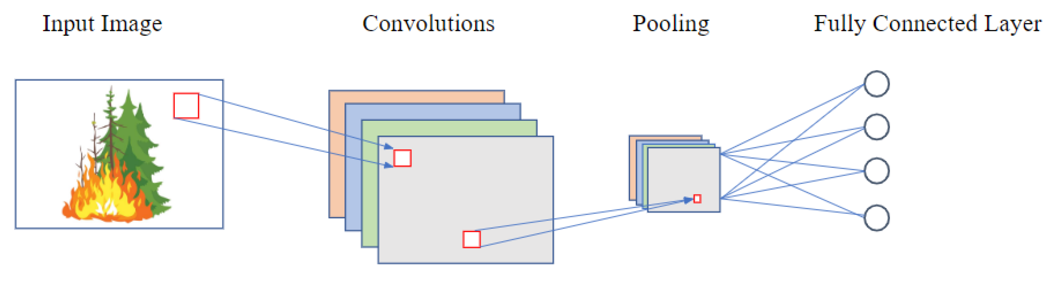
1.2.1. Convolutional Neural Networks

Convolutional neural networks (CNNs) are a subset of Artificial Neural Networks (ANNs) which exist for the purposes of image recognition, classification, and segmentation. CNNs distinguish themselves from ANNs by integrating contextual information by limiting connections to a receptive field [26]. This dramatically reduces the computational burden in order to handle larger images and avoid overfitting. Figure 1 depicts the structure of a 2D convolutional neural network consisting of three parts, a convolutional layer, pooling layer, and fully connected layer.

The convolutional layer performs the majority of the computation. In it, a kernel, or 2D matrix of learnable parameters, moves across the image preforming the dot product on a receptive field. The kernel moves across the whole image, producing an activation map. An activation map is generated for each channel within an image which acts to detect features within an image. Kernels can be tuned to increase or decrease their field of view, and more accurately fit the image with parameters of stride and padding. Stride defines how many pixels the kernel shifts by as it moves across the image. Increasing the stride decreases the resolution of the resulting activation map. Padding is used to retain borders of the image during the convolution, an unpadded convolution reduces the size of the feature map by the following function. Padding is often not used with large images, but with smaller images with important features at the borders. Lastly, a non-linear activation function is applied to introduce non-linearity to the linear convolution operation. This is carried out in order to preserve nonlinear features within the image. Popular activation functions are the sigmoid function, or the rectified linear unit (Relu). The pooling layer functions to reduce the number of parameters in the network, while retaining important feature information. A commonly used method for pooling is known as max pooling wherein the highest value within a filter is used for the output map. Other operations can be performed during pooling such as sum and average. The fully connected layer operates to take the lower dimensional feature output by the pooling layer and computes a non-linear combination of them. This allows the data to be classified, essentially creating a representation between the input and output data.

1.2.2. Image Segmentation and CNNs

In classification tasks, CNNs are typically used to predict a class of a whole image. However, image segmentation takes this concept further by using CNNs to predict classes for a given image on a pixel-by-pixel level. This technique is extremely useful for classification tasks in EO due to images rarely containing only one class, and where context within an image is important [12]. Figure 2 presents an example of multiclass image segmentation in the context of land with several land cover classification [27].

1.2.3. Encoder-Decoder Architecture

An encoder-decoder architecture takes CNNs one step further by up-sampling the CNN output feature maps to input resolution to preform pixel by pixel classification. The encoder can be seen as a traditional CNN which serves to extract feature maps. The decoder makes use of these feature maps, along with spatial information from earlier stages in the model through what is known as skip connections, this process combines more spatially accurate information with up-sampled features extracted from the CNN backbone. The advantage of being able to connect precise spatial information with the extracted feature maps dramatically increased the ability of CNNs. This technique is used widely in nearly all domains of deep learning from segmenting medical imagery to earth observation data. U-Net was originally developed by [28], the original encoder-decoder architecture utilizing skip connections in conjunction with deconvolutions within the decoder.

1.3. CNNs and SAR in Burnt Area Mapping

CNNs have been successfully applied to BA mapping applications, though nearly all are applied to multispectral imagery alone. Although successful, these studies focus on retrospective BA analysis, not real time. Further, these analyses are conducted with data collected in optimum MSI condition (e.g., cloudless skies) to achieve their results, something that is impossible during a real time wildfire scenario. Segmentation results in these studies achieve high overall accuracy (>0.95) scores but are limited in their applicability to real time BA mapping. This study aims to focus on the burgeoning field of BA mapping with SAR data instead, in combination with modern deep learning frameworks.

Only recently have studies begun combining SAR and modern deep learning architectures to attempt near real time segmentation of BAs during wildfires. Ban et al., 2020 [11] utilize Sentinel-1 C band imagery with image labels derived from time series change detection and a traditional CNN architecture to show it is possible to approximate BAs using SAR change maps, topography, and historical SAR data. The study is unable to determine accuracy over the whole study’s areas due to lack of accurate ground truth. However, they do propose a novel framework for anomaly detection in SAR time series data, which is implemented in this study.

Several studies have combined SAR and MSI with success in BA assessment [10,11,12,13,14,15,16,17,18,19]. Verhegghen et al., 2016 [19] show that the combined use of Sentinel-2 MSI and Sentinel-1 SAR can be utilized to detect and monitor fire outbreaks. The authors note the two technologies were able to compensate for the weakness of each other, but the study is limited in its geographic scope and specificity. They do not investigate the accuracy of their proposed technique beyond intersection and agreement of BAs between the two sensors.

Belenguer-Plomer et al., (2021) [29] utilize SAR and MSI images in a wall-to-wall mapping strategy to eliminate gaps caused by cloudy MSI imagery. They construct several CNNs to determine optimum model performance by land cover type. They found slightly higher accuracies when mapping BA with MSI data incorporated with SAR. The study notes marked differences in accurate results by land cover class, with heterogeneous land cover achieving the highest accuracies, and homogeneous land cover, such as cropland, achieving no addition benefit from the sensor combination. The study suffers from error sources stemming from steep topography, fire unrelated land changes in their study areas, and sparse fire events. The study does not investigate all land cover classes for a study area in a classification iteration. Zhang, Ban and Nascetti, (2021) [21] investigate continuous learning with a U-Net architecture exploiting both Sentinel-1 SAR and Sentinel-2 MSI time series for increasing the frequency and accuracy of wildfire progression monitoring. The study implements a frozen pre-trained ResNet encoder and trained decoder to refine burned areas in a progression-wise manner. This study shows the potential of deep learning as data becomes available at higher frequencies. The study fails to show the transferability of the method across land cover types and does not validate the models on BAs outside of their 3 case studies. This study aims to improve upon the ability of SAR-only based BA prediction models and investigate the potential of transfer learning in the subject. Specifically, it will address a gap left by other studies in incorporating other data into the deep learning process. Studies have largely ignored incorporating topography characteristics and land cover data into the learning process. There is strong theoretical ground for inclusion, yet many studies rely on SAR backscatter channels alone, due to lack of consistent data coverage. Another area neglected in the literature thus far is the area of transfer learning. The literature is sparse on the ability of any kind of machine learning model coupled with SAR to accurately predict BA once retrained on a new locality. This ability would represent a crucial step forward in being able to track BA progression across varied terrain and geography, though research has not yet fully evaluated this capability. Belenguer-Plomer et al., (2021) [29] train land cover specific CNNs to detect BA, though do not test their effectiveness combining land cover. This study aims to investigate both of the above gaps in the literatur-inclusion of additional data channels, and effectiveness of transfer learning in burn area monitoring. This work aims to contribute to the deep learning applications to SAR imagery in the context of near real-time BA mapping. The main objective is to determine if a modern deep learning architecture is an effective option relative to existing SAR based BA monitoring studies, as well as whether implementing a semi-supervised, automatic labeling process is effective in producing accurate predictions.

The specific aims and objectives of this study are: (1) to understand existing methods for semantic segmentation with respect to land cover classification and disaster monitoring; (2) to apply change detection technique to automatically label BA regions of Sentinel-1 and Sentinel-2 for fire regions in California; (3) to collate existing similar BA prediction models for comparison; (4) to apply a deep learning architecture for training and testing on labeled Sentinel-1 imagery and to evaluate contributions of additional channels (i.e., DEM and land cover); and (5) to evaluate model performance against existing Sentinel-1 based machine learning models for BA prediction, examining possible extensions with SAR and optical based fusion masks.

2. Materials and Methods

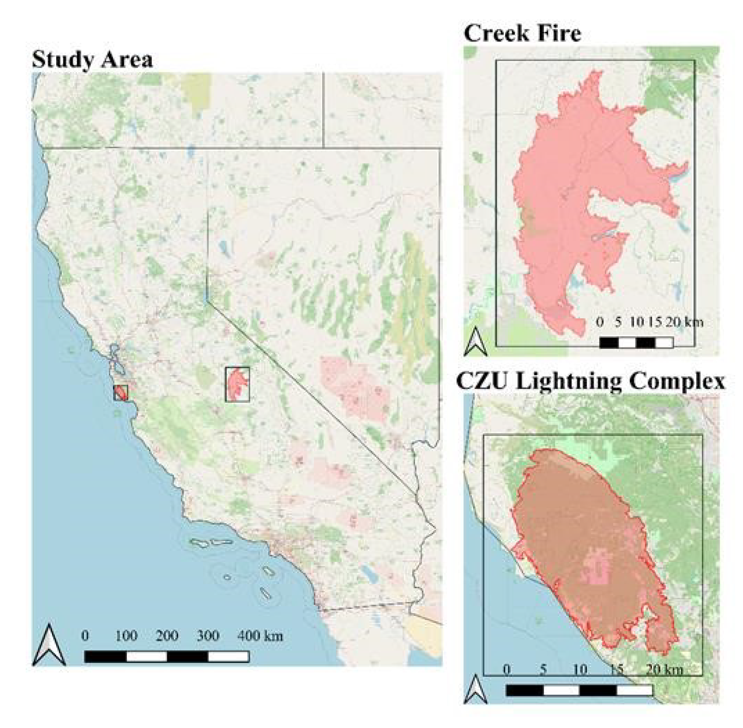
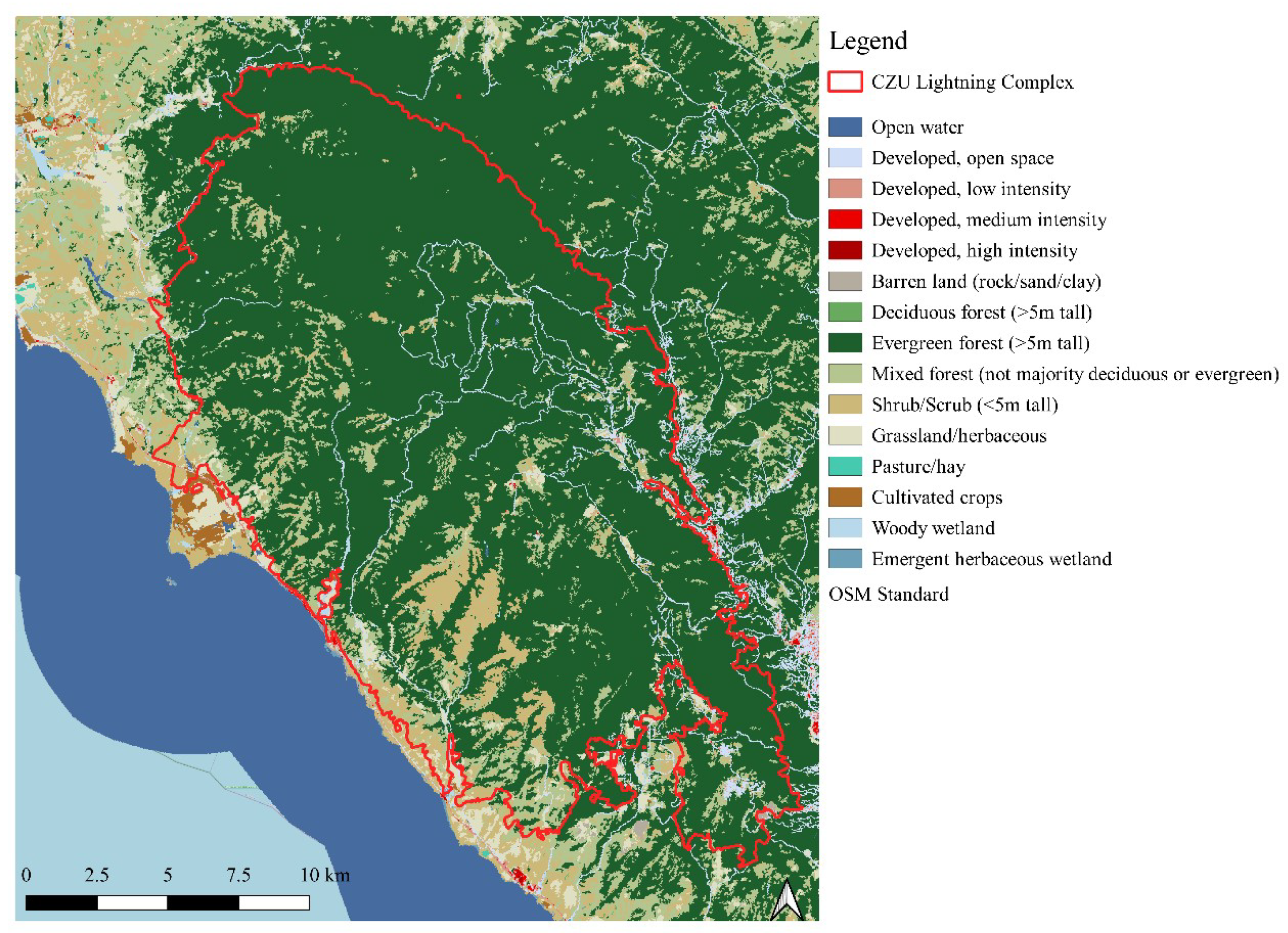
A summary of methodological steps is presented in Figure 3. After having identified a suitable study area with forest affected by wildfires, we cross checked Sentinel1 (S1) and Sentinel2 (S2) data availability for the time period using Google Earth Engine (GEE). Data Collection and Image Generation involved the download and clip S1 and S2 data for specific study area and time period. Generate CNN input data and pseudo label masks using S1 data automatic segmentation. After, we generated ground truth labels with S2 MSI data and CALFIRE reference outline. Model training has implied the CZU Lightning Complex model iterations on 11,600 fire event images and pseudo reference masks. Model testing was carried out using MSI ground truth reference. Additional transfer Learning was carried out by retraining the CZU models on Creek Fire SAR input data and pseudo labels, and test on MSI ground truth reference for the Creek Fire. Finally, a comparison of results of the three models to state-of-the-art SAR-based BA detection. We analyze the effect of the addition of ancillary non-SAR channels to the BA prediction accuracy.

2.1. Study Area

Two recent wildfires, the CZU Lightning Complex (2020) and the Creek Fire (2020), were chosen as case studies for this research due to the availability of previous application of radar remote sensing and deep learning for the mapping soon after the events. Figure 4 presents a map of each study area and

Table 1. Summary of Creek Fire and CZU Lightning Complex burnt area characteristics.

Creek Fire
Dates Active: 4 September 2020–24 December 2020
Total Area: 379,882.25 Acres
Location: 37.19147° N, 119.261175° W
Buildings Destroyed: 856
CZU Lightning Complex
Dates Active: 16 August 2020–24 September 2020
Total Area: 86,553.5 Acres
Location: 37.17162° N 122.22275° W

summarizes key characteristics about each. As the aim of this study is to investigate the transferability of a deep learning fire-monitoring model, both BAs presented similarities such as the presence of highly variable terrain, characterized by steep slopes and varied elevation, and similar land cover dominated by forest land (with a small fraction of forest class covered by shrubland/chaparral). On the other hand, the extent of the BAs was substantially different, as the BA of CZU Lightning Complex in nearly four times smaller than that of the Creek Fire. Combined, they are representative of wildfire events that occur within fire prone areas of California and contain characteristics, which are typically involved in large fires in recent periods.

2.2. Data

2.2.1. Copernicus Sentinel-1 SAR

Copernicus’ Sentinel-1 satellite program consists of a constellation of two polar-orbiting satellites launched in April 2014 and April 2015. They are both equipped with C-band SAR (active day and night) operating on a 6-day revisit period to the equator when using both satellites [30]. With these satellites, the ESA’s mission is to increase revisit frequency, spatial coverage, while providing additional SAR data for seas and oceans, natural hazards and disaster, and climate change monitoring [30]. Users can download SAR data as soon as one hour after acquisition in one of three levels. Relevant to this research is the Ground Range Detected (GRD) segment of Level-2, which consists of focused SAR data that is multi-looked and projected to the ground using an earth ellipsoidal model. High-resolution imagery (10m) is available in the interferometric wide (IW) swath mode.

The rise of cloud-processing systems, for instance Google Earth Engine (GEE), providing free of charge access to EO datasets worldwide [31], is promising. Therefore, it has been widely applied during the last decades [32,33].

From GEE, Sentinel-1 C band SAR data is downloaded for the period from four months preceding and two months after each fire event [31]. The GRD product in both VV and VH polarizations are downloaded in IW mode for the ascending or descending orbit, depending on swath coverage, aiming to prioritize as much of the study areas within a single swath as possible. Data for either an ascending or descending orbit is selected due to concerns of differences in azimuth angle and the affect it would have on data consistency over the same area.

The SAR data is processed according to the analysis ready processing guide provided by [34] for Sentinel-1 SAR data processed in GEE. Boarder noise removal, speckle filtering, and radiometric terrain normalization are implemented. Boarder noise removal is implemented in accordance with Stasolla and Neyt (2018) [35] due to its ability to be applied to data acquired regardless of acquisition mode, polarization, or resolution. Multi-temporal speckle filtering is applied with a Refined Lee filter using nine images and a 3×3 kernel [36]. Consistent with the analysis ready processing guidelines only areas of the same geometry are considered, and post speckle filtered images are manually checked against pre-filtered images to check adequate preservation of features. Radiometric terrain correction is conducted using the 30m SRTM DEM from NASA [37]. Terrain correction is essential for SAR data due to pronounced layover and shadow effects in areas with steep incidence angles. In this study, pixels in active layover and shadow zones are masked out in each image, in accordance with Mullissa et al. (2021) [34].

2.2.2. Reference MSI Imagery

Reference MSI imagery comes from the Sentinel-2 bottom of atmosphere product (2A) and is also downloaded from GEE. MSI images are downloaded for the same time period as the SAR and is used to define the final reference fire perimeters, described further below. Sentinel-2 images are collated together to form a continuous time series. For each BA a pre-fire and post-fire MSI image is chosen to facilitate the dNBR calculation. Cloudless pre-fire images are manually selected for both study areas as close to the fire start date as possible. Post-fire reference images are selected by selecting cloud free images at dates on or as close as possible to the conclusion of the fire event. In the case where a SAR and MSI image is not available on the same day, the closest acquisition dates possible are used. This is viewed as acceptable because at the point of data acquisition, the fire has reached it maximal extent, therefore data quality is prioritized (i.e., ensuring the image is cloud free). The NIR and SWIR bands are extracted and used to compute the NBR, forming the BA ground truth images for the U-Net model.

2.2.3. DEM

Topography data was obtained from the STRM 30m DEM in GEE, the same data as used in the radiometric terrain correction [37]. Separate slope, aspect and elevation layers were extracted for model input.

2.2.4. Fire Perimeters

The official CAL FIRE BA perimeter for each fire event has been obtained from the CAL FIRE data portal in conjunction with the MSI imagery to form the ground truth reference data (CALFIRE GIS Data, 2021) [38]. The perimeter is necessary to define the boundaries of the fire-affected areas, although it does not represent the heterogeneity within the burned area space, to do so, MSI imagery has been used to fill this gap.

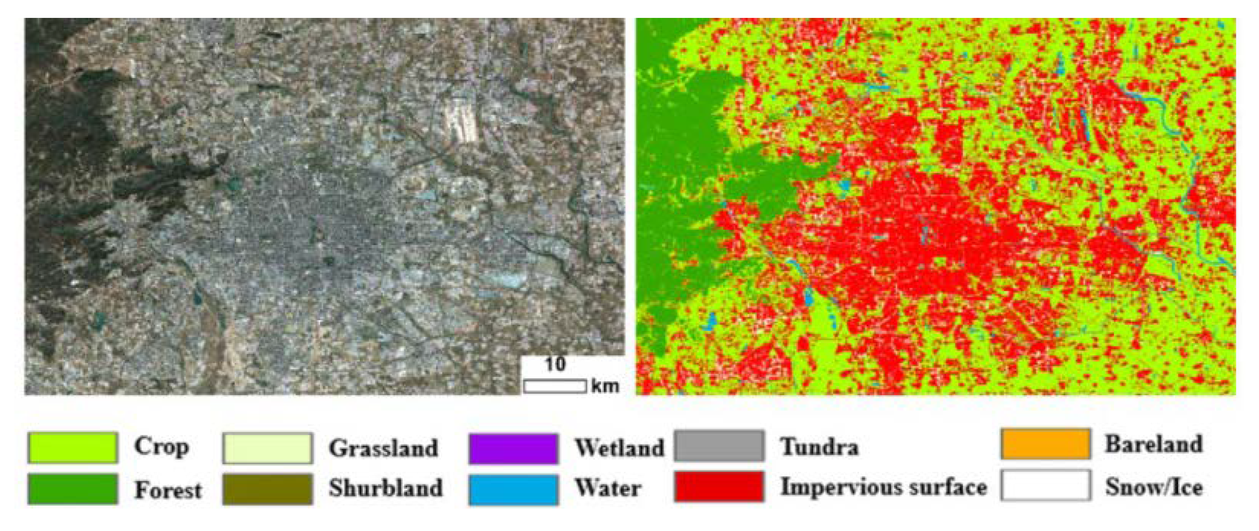
2.2.5. Land Cover Data

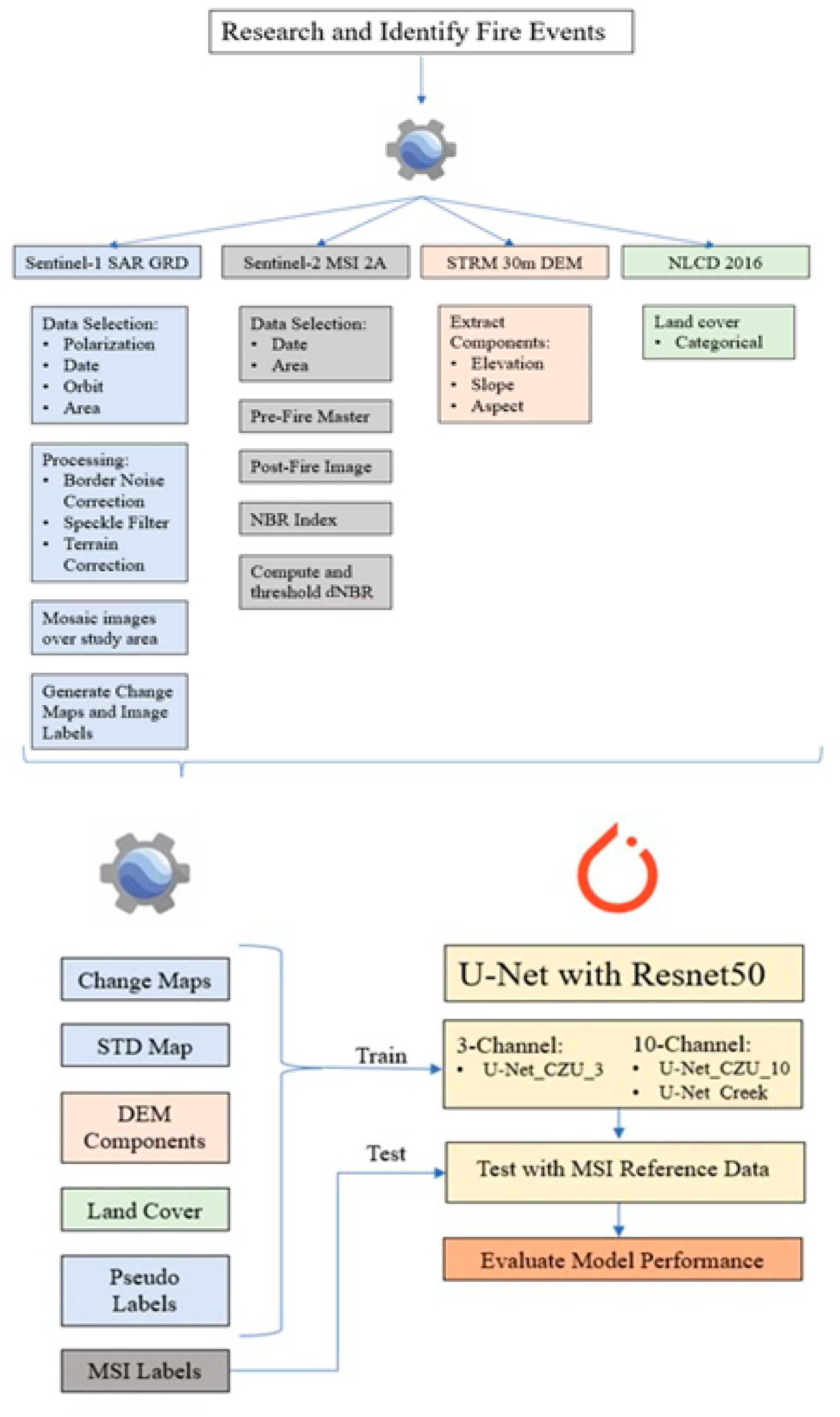
Land cover data used was originated from the USGS National Land Cover Database, which derived by the 30-m Landsat based imagery from 2016. It contains 20 cover classes and extends over both study areas completely. The data was downloaded via GEE.

2.3. Methods

The methodology for this analysis, builds upon the methodological framework proposed by Ban. et al. (2019) [11]. It contains two primary aspects: automatic input data and label generation via SAR change detection, and a semi-supervised deep learning model. Figure 5 summarizes the data components, brief processing, and flow of data into the modelling framework. The following sections will detail steps necessary related to SAR image anomaly detection and image pseudo labeling, input data processing, MSI ground-truth reference image generation, and the U-Net model specifications and modelling framework.

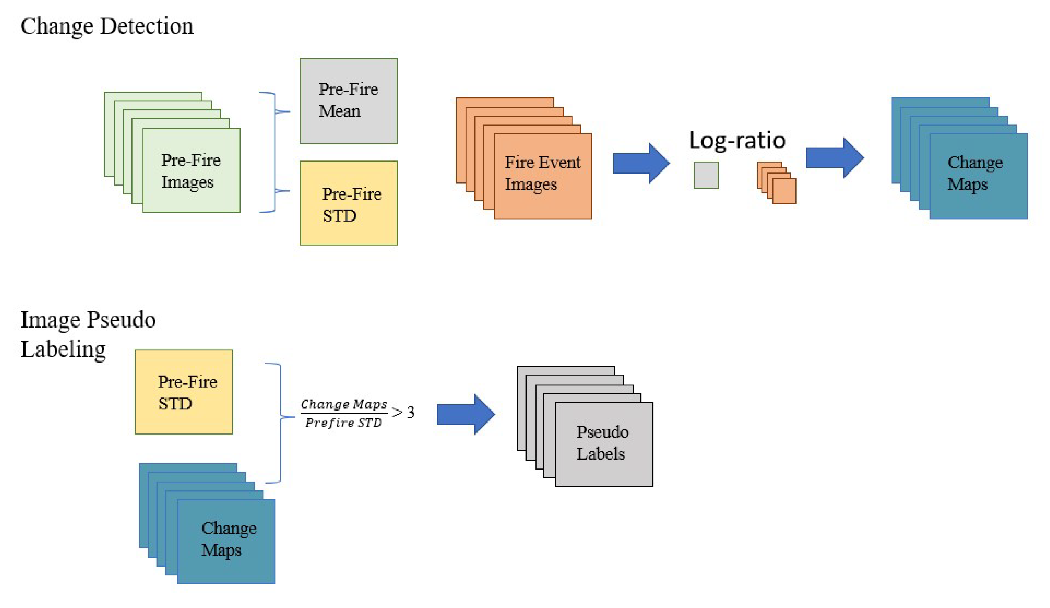
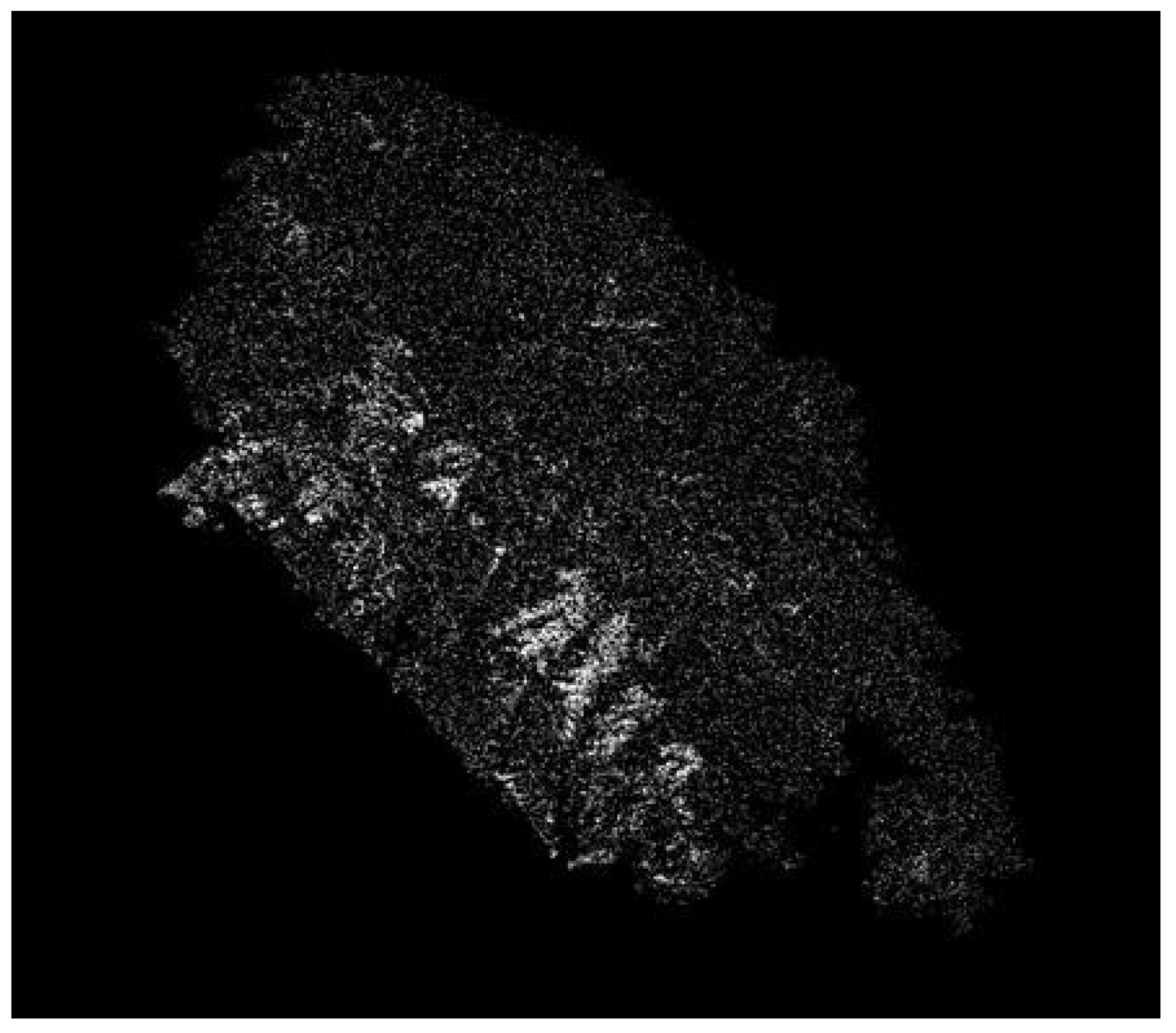
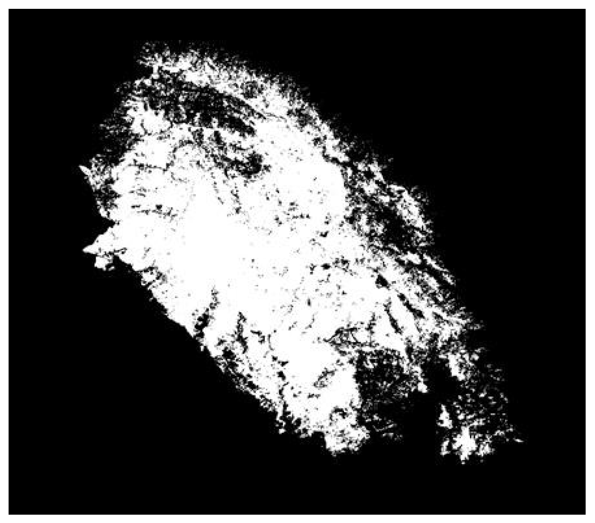
2.3.1. Change Detection and Image Pseudo Labeling

The method for anomaly detection and image labeling is described in Figure 5. Consistent with the framework of Ban et al. (2020) [11], SAR change detection is implemented by comparison of a pre-fire time series and post-fire image. For a given fire event, four months of pre-fire SAR images are collected and processed according to the analysis ready data protocol laid out above. From these images, a historical pre-fire mean and standard deviation image are produced for each VV, VH, and VV/VH polarizations. These images define a pixel wise reference for what a normal backscatter range is for each study area. Change maps are derived from the pre-fire time series by calculating the log ratio between a post-fire image and the pre-fire mean. The formula for the log difference is presented in Equation (4) [39].

Equation 4: Formula for log ratio between two SAR images.

$$X_{LR}=log\left(X_R\right)=log\left(\frac{X_2}{X_1}\right)=log\left(X_2\right)-log\left(X_1\right)$$

(4)

where X_LR is the resulting loss ratio image, log X₂ is the post-fire image, and log X₁ is the pre-fire mean. Here, the log difference can be seen as calculating the degree of difference between the two images. The time series of individual SAR polarization change maps is the primary component of the input data. From the change maps, the pseudo labels are generated by dividing the change maps by the pre-fire standard deviation image, presented in Equation (5) [11].

Equation 5: Formula for degree of deviation from normal for a SAR image.

$$D_{pix}=\frac{\left|X_{LR}\right|}{Im{g}_{STD}}$$

(5)

D_val represent the deviation from normality for each pixel in the change map image, |X_LR| is the absolute value of the change map, and Img_STD is the pre-fire standard deviation map. The larger the deviation value, the higher the probability of change. Due to speckle in the image, we found it difficult to distinguish a hard line between BA and noise in the data. However, through manual thresholding of the deviation value, we identified a balance between BA detection and noise in the data.

The resulting threshold is equal to three. Using this threshold, the change maps are binarized and clipped to the final fire perimeter (provided by CAL FIRE). Clipping is carried out to minimize false positive labels in the data. Though this step would be unsuitable in a real time detection situation, this study seeks to maximize BA detection with SAR. The resulting deviation maps are used as input pseudo labels for training the deep learning algorithm. An example of a derived image pseudo label is presented in Figure 6, for the CZU Lightning Complex study area.

2.3.2. MSI Reference Images

Ground truth image labels are generated from MSI imagery derived from Sentinel-2 imagery. NIR and SWIR bands are used to calculate the NBR for each pre-fire master image and post fire burnt image for each study area. Only one burnt image each is used to serve as a ground truth reference because Sentinel-2 data is unavailable while the fires are active.

Similarly to anomaly detection in SAR, a pre-fire NBR and post-fire NBR are differenced to produce a differenced NBR image (dNBR), which, after thresholding, serves as the ground truth reference for the final fire perimeter. Thresholding of the dNBR is carried out in accordance with the Monitoring Trends in Burn Severity (MTSB) program, in which a dNBR threshold of >.1 is used to identify all burnt severities above unburned levels [40]. This is a common practice in BA detection and has been shown to detect over 97% of BAs for boreal forests, which is viewed as sufficient for this study [11,12,13,14,15,16,17,18,19,20,21,22,23,24,25,26,27,28,29,30,31,32,33,34,35,36,37,38,39,40,41,42]. The binary BA reference map is presented below for the CZU Lightning Complex fire in Figure 7. This BA reference is not used to train the U-Net models, but solely used in assessing accuracy of the proposed U-Net for BA detection.

2.3.3. U-Net Input Data Summary

The final input dataset used to train the U-Net consists of either three channels or ten channels. The three channel iterations consist of only the three SAR polarization change maps. The ten channel iterations consist of the three polarization difference map channels, three polarization pre-fire standard deviation channels, DEM components, and land cover classification. The change maps and standard deviation are included with three layers each, of VV, VH, and VV/VH. This is due to polarizations picking up different aspects of the Earth’s surface, with VH being most susceptible to volume scattering within a tree canopy. The DEM components include slope, aspect, and elevation. Land cover classification is a raster of categorical values provided by the USGS national land cover database. Each input channel is stacked and exported into a single three or ten channel “.tiff” file at ten-meter resolution from GEE.

2.3.4. Input Dataset Manipulation

As the U-Net requires images of height and width of 128 X 128 pixels, a splicing algorithm was used to split the tiff files into patches of the required size to retain resolution. In total, for the CZU study area, 725 images are available for each instance of data acquisition. For the CZU fire event, 11,600 input and pseudo reference images are available for training during the fire period and 725 MSI generated images were used for testing. This equates to training on the first 16 instances of data acquisition during the fire period and testing on the final instance, i.e., when the fire reaches its full BA perimeter. Each channel within each input image is min-max scaled to be between 0–1 based on the global minimums and maximums throughout each respective dataset. This process helps the U-Net converge more quickly by reducing volatility in the data. At the conclusion of testing the predicted image, patches are reassembled for statistical and visual accuracy comparison with the reference imagery. Specific accuracy metrics are shown in Section 3.1.

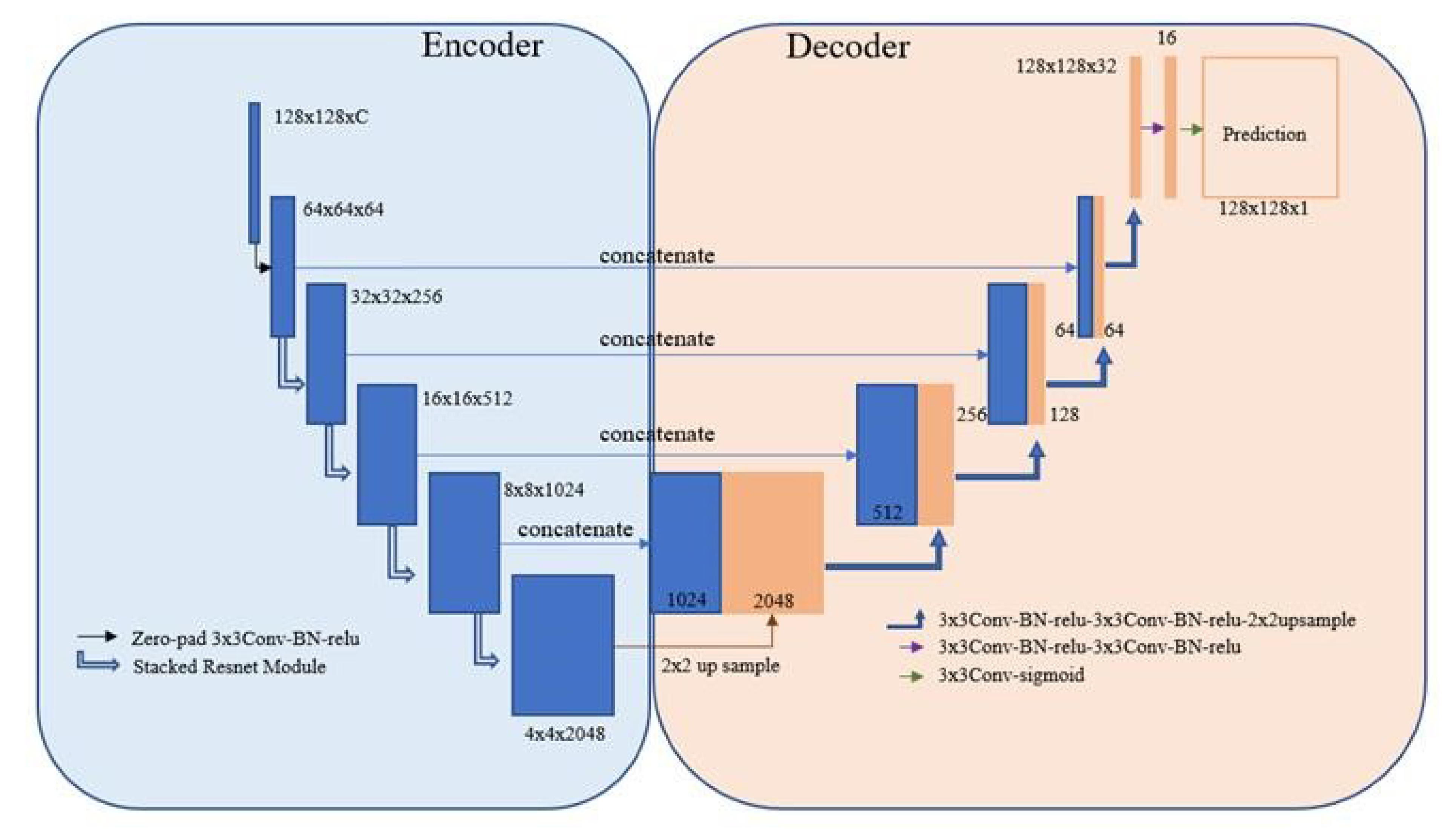
2.3.5. U-Net with ResNet

Deep neural networks have demonstrated great successes in segmenting earth observation data. However, deep networks often suffer from the problem of being very unstable. This is known as the exploding or vanishing gradient phenomenon, where errors propagate into very large updates, rendering the network useless. Researchers solved this problem with implementation of so-called skip connections which are composed of a mapping of previous layers in the network [43,44]. For segmentation tasks, Ronneberger, et al., 2015 [28] propose a novel encoder-decoder framework applying some of the similar principles. The U-Net consists of a contracting path and expanding path with concatenations at corresponding levels between the encoder and decoder. The advantage of this structure is that it retains contextual information while also including low-level detail. It has been shown to be very effective in segmentation tasks, including in EO. In this study, the U-Net and Resnet were combined to exploit the advantages of each framework. Specifically, a ResNet50 encoder was incorporated as the encoder of the U-Net. ResNet50 was chosen specifically based on its successes in BA mapping in previous studies together with other encoder-decoder architectures [21]. The architecture for this study is illustrated below in Figure 8.

2.3.6. Models

This study presents three deep learning models that were trained for the evaluation of BA monitoring. The model specifications implemented here are listed below:

U-Net CZU_10:

• The U-Net model is loaded as an untrained model with randomly initialized weights for each of the 10 channels. The model is then trained on the 11,400 image patches specific to the CZU BA of interest. The model is tested on 725 images representing the final BA at the conclusion of the fire.

U-Net CZU_3:

• Take only the dVV, dVH, dVV/dVH SAR polarizations as channel inputs to a 3-channel U-Net using the ImageNet pre-trained weights. It is then trained on 11,400 image patches and tested on the 725 image patches of the final BA perimeter.

U-Net Transfer:

• Load the weights from U-Net CZU_10 and continue training the model on a subset of images from the Creek fire. This is intended to learn from the initial training and generalize it to an area of similar land cover and topography in California. Investigate effects of additional land cover and topography channels in transfer learning.

2.3.7. Model Training

Each model presented in the study has been trained with parameters specific to the input data. This section will detail the specific data treatments and hyperparameters utilized during the training process for each model listed above.

Data Augmentation

During training of both U-Net CZU and U-Net Transfer models, data augmentation has been implemented to deliberately increase the diversity of characteristics within the dataset. This has been carried out to allow the network to generalize more readily with a relatively small amount of training data. Specifically, augmentations consist of Gaussian noise on one fifth of images and reorienting images half of the time.

Hyperparameter Tuning

In this study, hyperparameters considered for tuning are the learning rate, number of epochs, and loss function [45]. Hyperparameter tuning has been performed on a smaller subset of data. In this study, tuning has been limited to a subset of 1000 images (~9% of the total data) due to training time constraints.

Table 2. Summary of model training hyperparameters.

Model	Rate	Epochs	Loss Function	Learning Optimiser	Training Set Size	Test Set Size
U-Net CZU_3	0.001	240	Dice Loss	Adam	11,600	725
U-Net CZU_10	0.001	320	Dice Loss	Adam	11,600	725
U-Net Transfer	0.001	320	Dice Loss	Adam	9699	1233

summarizes the model hyperparameters.

Learning Rate

The learning rate governs the size of the weight updates. If the weight updates are too small the model never converges, too large, the model will overshoot the minimum. The learning rate has been found to be optimized at 0.001. This determination has been made by looking at the training curves after the conclusion of each tuning training model run, making sure the curve is not too jagged, or not learning fast enough.

Number of Epochs

The number of epochs to train each model is determined based on the relationship between the training and validation loss curves. As training progresses both training and validation loss decrease. At a certain point, validation loss begins to increase relative to training loss. This point is understood as the point at which the model begins to overfit the training data. This epoch is identified, and the validation data is re-included in the training set. The model was trained for the found number of epochs. The training epoch with the lowest dice loss during the training period was the one chosen for the test.

Loss Function

The loss function determines how well a model fits input data based on the output of the prediction, compared against the ground truth. Different loss functions are used based on the type of data being analyzed. Data components such as class distribution, skewness, and boundaries govern what kind of loss function is implemented. Popular loss functions are Cross Entropy loss and Dice Loss [45].

The loss function used in this study for all models is Dice Loss. Dice Loss was chosen because it is shown to handle class imbalance and outliers more smoothly than cross-entropy, and also because it has been applied in BA estimation previously [10,29]. Further, it is based off this study’s evaluation metric, the F1-score, so minimizing the Dice Loss it maximizes model performance.

2.3.8. Model Evaluation

In the space of EO, segmentation models were evaluated by accuracy metrics. In accordance with the field, this study will compare accuracy metrics to other papers in the field of BA estimation with SAR. Additionally, this study will examine some qualitative aspects of the segmentation in an attempt to identify meaningful trends as to why prediction succeeded or struggled.

Evaluation Metrics

Quantitative metrics were used to evaluate performance of both BA segmentation models consist of the Accuracy, Precision, Recall, and F1-score. The evaluation metrics are defined in

Table 3. Evaluation metrics presented in this study.

Metric	Formula
Sum of all burnt area pixels	True Positive (TP) classified as burnt area
Sum of all burnt area pixels	False Positive (FP) classified as unburned area
Sum of all unburned area	True Negative (TN) pixels classified as unburned area
Sum of all unburned area	False Negative (FN) pixels classified as burnt area
Accuracy	$\frac{TP+TN}{TP+TN+FP+FN}$
Precision	$\frac{TP}{TP+FP}$
Recall	$\frac{TP}{TP+FN}$
F1-Score	$2\frac{Precision * Recall}{Precision+Recall}$

. The metrics are consistent and correlated with each other and are regularly used in the literature. Since this study is comparing performance against studies in the field, it is necessary to use comparable statistics. Importantly, this study will only compare to other studies using a consistent technique.

Benchmark Studies

As the field of SAR-only BA detection is relatively new, there does not exist any official benchmark to assess this study’s findings against. There are a few recent studies, however, undertaking analysis of SAR-based BA prediction and deep learning that will be used to evaluate the findings in this study. The comparison studies are Belenguer-Plomer et al. (2021) [29] and Zhang, Ban and Nascetti (2021) [21] which both implement CNN based SAR only BA estimation models. Both studies utilize a similar approach of SAR change detection to generate change maps of affected areas, which are then used to train a machine learning model. In terms of study area, comparisons are made against similar geographic regions where possible. Belenguer-Plomer et al. (2021) [21] provide assessment of a BA in Northern California, which is geographically close to those presented in this study and is chosen as the point of comparison. Zhang, Ban and Nascetti (2021) [21] provide a SAR-only based model for their Sydney, Australia BA, though land cover and topography are broadly consistent this study (70% evergreen forests, ~10% scrubland over hilly and mountainous terrain). Trained models are tested on ground truth reference generated with a methodology consistent with this study. Belenguer-Plomer et al. (2021) [29] utilize Landsat-8 surface reflectance and a random forest classifier trained on 1) NIR and SWIR bands 2) the NBR of post-fire and 3) the pre- and post-fire NBR (dNBR). Consistent with this study Zhang, Ban and Nascetti (2021) [21] utilize a threshold dNBR approach to derive the reference perimeters from Sentinel-2 and Landsat-8 MSI imagery. The dNBR threshold used to define BA is the same as implemented here (>0.1). Both studies evaluate the ability of SAR-only based BA prediction models and SAR-MSI based BA prediction. This study only considers the former in the evaluation comparison but does address the latter in discussion.

Table 4. Summary of benchmark study results for SAR based burn area detection ¹ Based on the U-Net with Learning without forgetting with SAR based reference for the Sydney Fire (2019-2020); ² Based on North American study area S1 satellites only.

Model	Accuracy	Precision	Recall	F1
Zhang Ban and Nascetti (2021) 1	0.86	095	0.45	0.60
Belenguer-Plomer (2021) 2	-	-	-	0.46

summarizes the results for the two comparison studies Belenguer-Plomer et al. (2021) [29] only provide F1-score for comparison).

All models presented are evaluated against the comparison studies. This study assumes that due to the relatively small amount of research into this specific area to-date, these comparison studies represent the state of the art in terms of SAR-only BA estimation.

Qualitative Evaluation

Together with the quantitative evaluation, a qualitative analysis is undertaken to determine which models work well in what landscapes. Qualitative analysis aims to determine if aspects of the land cover or topography notably challenge the BA estimator. Of particular interest are the mountainous regions of the study sites as SAR traditionally struggles in mountainous terrain. Qualitative analysis is conducted by visually inspecting the error regions of each predicted BA for particularly dense regions of false negatives and false positives.

3. Results

The section presents results and evaluation of performance for each BA prediction models, presented by study area. The models were evaluated with traditional accuracy metrics for image segmentation listed in Table 3 and compared against the benchmark studies listed in Table 4. A brief analysis was conducted to assess successes and struggles of the models in the CZU study area regarding land cover and topography.

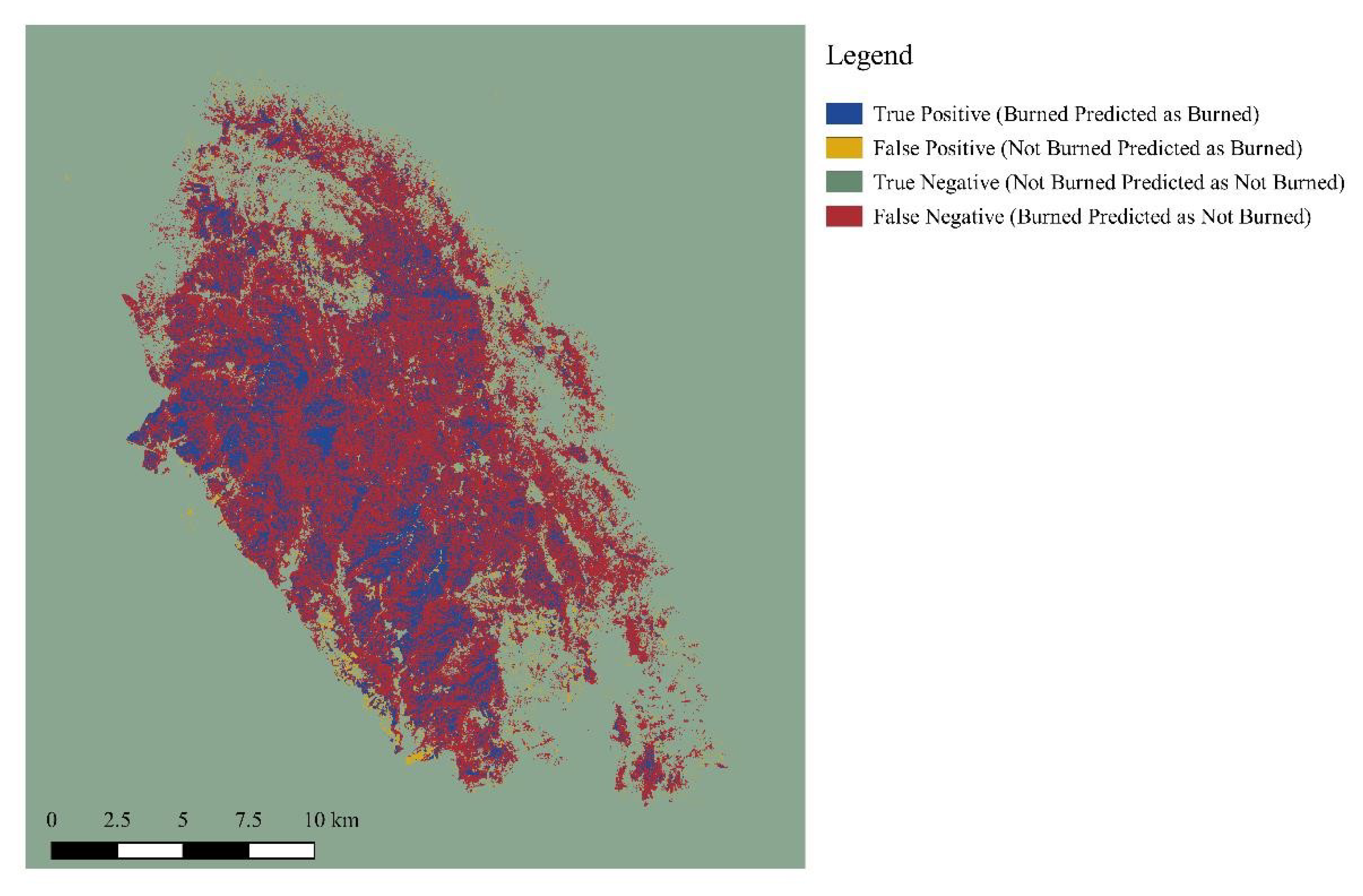
3.1. CZU Lightning Complex

Table 5. CZU Lightning Complex U-Net Segmentation Results.: ¹ Based on the U-Net with Learning without forgetting with SAR based reference mask for the Sydney Fire (2019-2020); ² Based on North American study area S-1 satellites only.

Model	Accuracy	Precision	Recall	F1-score
Zhang, Ban and Nascetti (2021) 1	0.862	0.947	0.448	0.604
Belenguer-Plomer (2021) 2	N/a	N/a	N/a	0.460
U-Net_CZU_3	0.813	0.868	0.650	0.671
U-Net_CZU_10	0.807	0.833	0.648	0.667

presents the results of the two models, U-Net_CZU_3 and U-Net_CZU_10, together with the literature studies and their performances. Figure 9 presents the visual segmentation result for the UNet_CZU_3 model. Errors, false positives, and false negatives can be observed highlighted in yellow and red. Blue and green represent true positives and true negatives, respectively.

Both U-Net CZU models achieve higher accuracies with respect to the metric of interest, F1score when compared to the two literature benchmarks. U-Net_CZU_3 records an F1 score of 0.671, U-Net_CZU_10 records an F1 score of 0.667, compared to 0.60, and 0.46 from Zhang, Ban and Nascetti (2021) [21] and Belenguer-Plomer et al. (2021) [29], respectively. As expected, the work of Zhang, Ban and Nascetti (2021) is the closest in terms of accuracy as the methodology is very similar to this study.

The U-Net was generally unsuccessful in categorizing much of the BA, though did a much better job at not categorizing unburned area as burned (Figure 9). The algorithm successfully categorizes BAs where the surrounding area is nearly completely burned, while it struggles to classify areas that go from burnt to unburned in succession over shorter distances. For example, a great portion of entire right edge of the figure was misclassified when it comes to the BA, though the lower left portions of the image are fairly better. While the two model’s classification performance metric is very similar there is noticeable difference in output image. Namely, U-Net_CZU_3 produced results with noticeably lower false positives in the lower right tail than U-Net_CZU_10. Additionally, based on the pattern of the classification, land cover and topography appear to play a role in this discrepancy of BA classification.

3.1.1. Land Cover Effects

The predominant land cover types for the CZU Lightning Complex are evergreen forest and small amounts of scrubland (Figure 10). Notably, the U-Net CZU seems to have classified accurately the shrubland inside the fire perimeter, though there is not a clear pattern with respect to the evergreen classification.

3.1.2. Topography Effects

Table 6. Topography summary statistics by prediction class for U-Net_CZU_3.

Metric True Positives	Mean	Min	Max
Elevation (ft)	369.80	−10.00	821.00
Slope (degrees)	17.40	0.00	69.50
Aspect (degrees from North) False Positives	181.25	0.00	359.50
Elevation (ft)	365.10	−6.00	918.00
Slope (degrees)	14.60	0.00	56.00
Aspect (degrees from North) True Negatives	168.90	0.00	359.30
Elevation (ft)	248.00	−12.00	996.00
Slope (degrees)	11.80	0.00	69.50
Aspect (degrees from North) False Negatives	164.20	0.00	359.70
Elevation (ft)	382.00	−12.00	821.00
Slope (degrees)	17.80	0.00	71.40
Aspect (degrees from North)	166.40	0.00	359.50

summarizes the topography variation amount the different U-Net CZU classifications. It is evident that the true positive metrics noticeably diverge from the false positives and true negatives, as one might expect. This suggests that the characteristics of land cover that were unburnt after the fire could be substantively different from those that are in the fire. Examining the region of interest, together with the final fire perimeter, this seems plausible. However, more research is necessary to make a definitive conclusion. Notably true positive and false negative (burnt predicted as not burnt) consist of very similar metrics. This too is to be expected given the relative consistency of the BA in terms of the DEM components. It does suggest, however, that the U-Net was not taught that the attribute is an effective differentiator between areas burned and not burned.

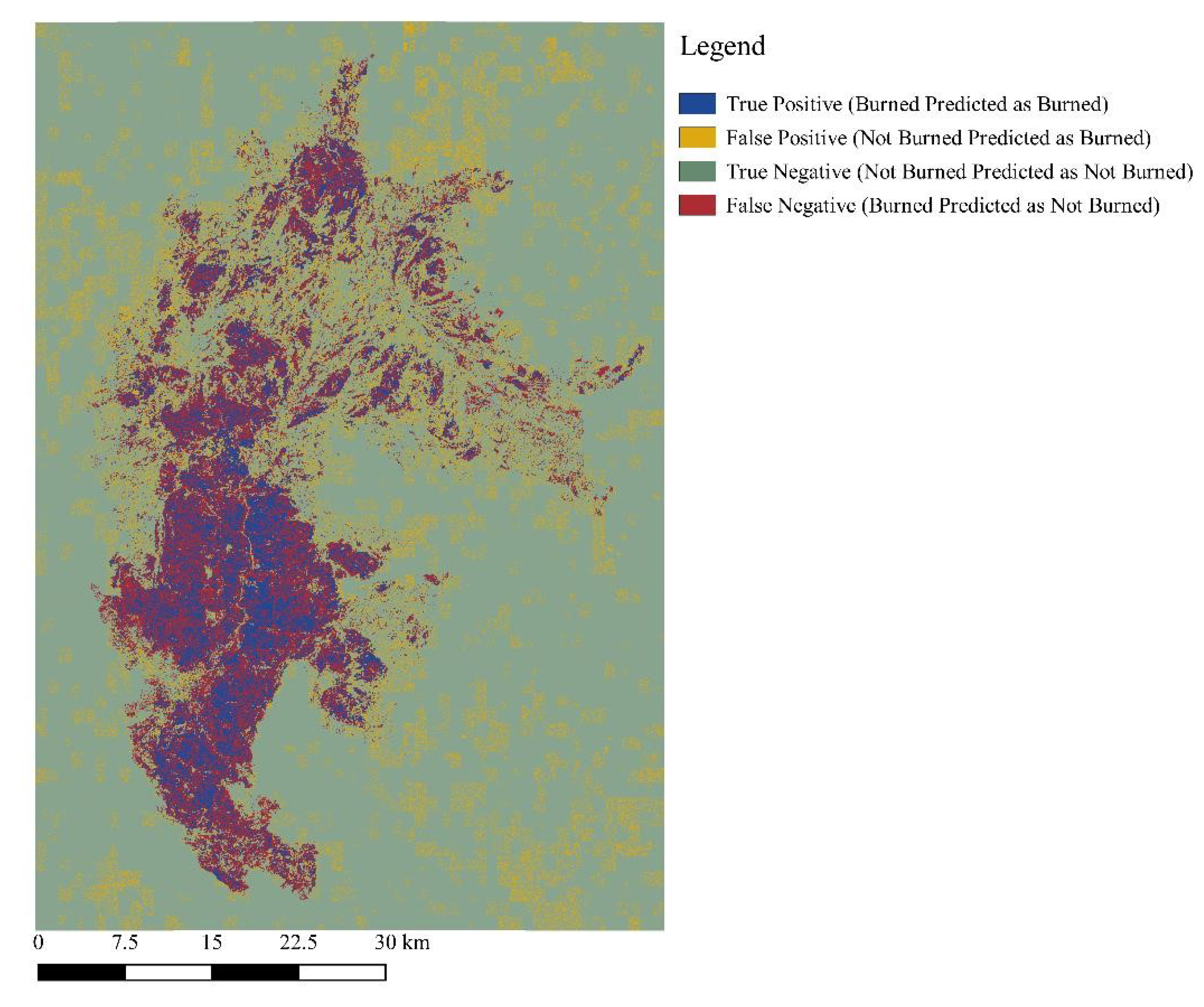
3.2. Transfer Learning of the Creek Fire

This section presents results of transfer learning in context of the Creek Fire study area. To accomplish transfer learning, U-Net_CZU_10 is retrained on 9,699 ten channels tiff images together with pseudo labels from the Creek Fire progression.

Table 7. Creek Fire Transfer Learning Segmentation Results: ¹ Based on the U-Net with Learning without forgetting with SAR based reference mask for the Sydney Fire (2019-2020). ² Based on North American study area S-1 satellites only.

Model	Accuracy	Precision	Recall	F1-Score
Zhang, Ban and Nascetti (2021) 1	0.862	0.947	0.448	0.604
Belenguer-Plomer (2021) 2	N/a	N/a	N/a	0.460
U-Net_CZU_3	0.813	0.868	0.650	0.671
U-Net_CZU_10	0.807	0.833	0.648	0.667
U-Net_Transfer	0.810	0.460	0.730	0.410

presents the results of for U-Net_Transfer with previous study models and benchmark study results. Transfer learning resulted in F1-score lower than those previously noted. After retraining the U-Net_CZU_10 model on the Creek Fire10-channel input data and pseudo labels, the resulting performance is an F1-Score of 0.41, compared to U-Net_CZU_3 F1-Score of 0.671 and the comparison studies, 0.60 and 0.46.

In Figure 11 the labels of the Creek Fire predicted BA are shown as predicted by U-Net_Transfer. The high-level shape is visually similar to the reference image. U-Net_Transfer demonstrates ability to accurately classify dense BAs in the center of the image. U-Net_Transfer struggles with edge detection, in contrast with either U-Net_CZU. Water bodies, including rivers and lakes, are generally classified well with U-Net transfer.

4. Discussion

This section provides a summary of the strengths and weaknesses of this study’s approach to BA mapping the context of Sentinel-1 SAR data. Further, it discusses the merits and challenges faced by each model in the study. Finally, implications for the field are discussed.

4.1. Data Labeling

The primary challenge of this study is the generation of accurate labels for each deep learning model to utilize. This is exceedingly difficult in the context of Sentinel-1 SAR data for multiple reasons, including data processing, subjective thresholding, and lack of ground truth during fire events. In this work, we attempted to find the optimal speckle filter through trial and error based on techniques found in the literature relevant to SAR. However, a clean image cannot be achieved. This challenge is not unique to this study and further research is necessary to find a more viable solution in the case of BA monitoring with SAR. Improving speckle processing capability for Sentinel-1 imagery would greatly enhance the ability of a deep learning model to classify BA, as evidenced by the results presented here. In all results from each model exists a persistent problem of noise, and poorly defined burnt limits, which is likely due to the noise in label creation. An additional challenging part of the work is the label creation, which is by its nature subjective and can depend on the change detection threshold. This study follows the pseudo label implementation of (Ban et al., 2020) [11], wherein a subjective threshold for the derived change map and MSI imagery is implemented. In previous SAR studies, this has largely been a balancing act between retaining BA features while reducing noise in the image. The higher the threshold set for change, the less noisy the image, though the BA features become degraded (manifesting primarily in discontinuous feature areas). Variability in this thresholding exercise is likely responsible for the large omissions in continuous BAs. The primary driver of label uncertainty is the actual unknown of ground truth. As mentioned previously, one of SAR’s great advantages is its ability to sense in conditions where optical sensor cannot. This leads to a problem in SAR label generation, though. Since I did not have ground truth reference while fine tuning the change detection thresholding, it is not possible to know how accurate the labels truly are. The solution this study implements is to base thresholding parameters off a period when MSI and SAR comparison is possible on a post-fire event date. This is viewed as acceptable though not ideal due to the inconsistency in the generated labels.

4.2. U-Net CZU Model Successes

Both U-Net_CZU_3 and U-Net_CZU_10 achieved higher F1-score than previous studies undertaking BA monitoring with Sentinel-1 SAR imagery alone. This success was driven by choice of model architecture, U-Net with a ResNet encoder, and choice of data sources, fire event change maps with additional pre-fire standard deviation, DEM, and land cover channels.

The area inside the CZU Lightning Complex fire perimeter was characterized by largely homogenous land cover of evergreen forest (>80%) prior to the fire event, this likely contributes to the success of more accurate classification with the U-Net_CZU_3. Although noisy, the SAR backscatter provides a uniform response during the fire event, which likely contributes to the model’s ability to distinguish more distinct edges and patches of contiguous BA. Given the homogenous nature of the land cover within the BA, it is likely other sources such as the variation in topography, i.e., slope and aspect, may play a larger role in influencing the inconsistency in the accuracy of the classification.

4.3. U-Net Transfer Challenges

The aim to show transferability between detection of fire events based on SAR change detection is largely unsuccessful in the context of this study. The model, U-Net_Transfer, delivered the lowest F1-scores seen in the study. The minor segmentation accuracy, however, does suggest that this approach has potential. The uncertainty and noise in the data and labels associated with both fire events likely contribute to the poor result. Retraining the model into U-Net Transfer does not generate results on par with the original U-Net CZU models, however. This could be due to the fact that the BAs of the two fires are markedly different. The CZU Lightning Complex is characterized by a smaller area of continuous BA, while the Creek fire is characterized by an area nearly four time greater with many tendril-like BAs. Given that the U-Net CZU models would have learned the context of densely burned areas initially, it is reasonable to think that it would struggle with a BA footprint that deviates from the pattern. This is supported by the dense area of correct categorization in the middle of the BA.

4.4. U-Net Model Limitations and Implications for Future Works

As with any deep learning model, the results can only be as accurate as the input data. This study is limited by inaccuracy and uncertainty in its input data as well as in the data labeling. U-Net and other deep learning models are known to be robust to noise in the data labels, though noise in the input data is notoriously challenging [46]. This study is limited by both imprecise input data, i.e., noise in backscatter change maps, and in the data label by the same method. The inconsistency in the BA result could have possibly been made worse by the introduced augmentations to data labels, though we chose to limit the potentially harmful augmentation, Gaussian blur, to a small (P = 0.2) amount of the data labels, hoping to retain some of the advantages. In line with prior research, this study finds that deep learning can be applied to SAR for BA prediction. This supports a promising step forward for active remote sensing technology that has the potential for substantive application in resource management, biomass monitoring, and environmental restoration. This study shows that additional factors such as land cover and topography have the ability to influence classification results, though not always positively, instead of just SAR backscatter data alone. This finding is important for future researchers to create robust segmentation model across similar regions. SAR for BA monitoring shows great promise in being able to complement its MSI counterpart in the near future, but speckle processing must be improved to achieve this performance. Even with current deep learning frameworks, improved speckle in images would dramatically improve pseudo labeling and improve prediction results. Due to the unavailability of the most detailed SAR data (largely from commercial providers such as ICEYE [47] and Capella Space), nearly all of the research in the field is limited to SAR with resolution of 10 m at best. Commercial data is now being acquired at levels <3 m and even <1 m in some applications. Research into how current analysis techniques pair with truly modern data is critical for a robust analysis framework once this high-resolution data becomes available. Additionally, the generalization of deep learning framework for SAR change detection has the potential to be improved by training frameworks on a database of fire events, rather than just a handful. This kind of generalization would be at the center of an always-on fire progression-monitoring tool.

5. Conclusions

This study has presented a GEE and PyTorch enabled framework for SAR data processing, automatic pseudo label and input data generation and an effective deep learning framework for Burnt Area (BA) classification.

The main conclusions of this study area as follows:

• Automatically generated pseudo labels used in tandem with an encoder-decoder network is an effective method to classify BAs during a fire event;
• Adding additional channels of topography and land cover affects the result of deep learning prediction using SAR imagery. In the case of this study, the effect was slightly negative;
• Transfer learning for BA monitoring is not as effective as first-time learning.

This reinforces the view that SAR backscatter is highly particular to peaks and valleys.

The results of this study contribute to the growing field of research in applications of SAR data for EO, and to an eventual improvement of the way resources managers respond to these devastating natural disasters.

References

1. Stefanidis, S.; Alexandridis, V.; Spalevic, V.; Mincato, R.L. Wildfire Effects on Soil Erosion Dynamics: The Case of 2021 Megafires in Greece. Agric. For. 2022, 68, 49–63. [Google Scholar] [CrossRef]
2. Silvestro, R.; Saulino, L.; Cavallo, C.; Allevato, E.; Pindozzi, S.; Cervelli, E.; Conti, P.; Mazzoleni, S.; Saracino, A. The Footprint of Wildfires on Mediterranean Forest Ecosystem Services in Vesuvius National Park. Fire 2021, 4, 95. [Google Scholar] [CrossRef]
3. Patel, K. Six Trends to Know about Fire Season in the Western U.S., Climate Change: Vital Signs of the Planet. 2018. Available online: https://climate.nasa.gov/blog/2830/six-trends-toknow-about-fire-season-in-the-western-us/ (accessed on 10 June 2021).
4. Anguiano, D. California’s Wildfire Hell: How 2020 Became the State’s Worst ever Fire Season, the Guardian. 2020. Available online: http://www.theguardian.com/usnews/2020/dec/30/california-wildfires-north-complex-record (accessed on 10 June 2021).
5. Schroeder, W.; Prins, E.; Giglio, L.; Csiszar, I.; Schmidt, C.; Morisette, J.; Morton, D. Validation of GOES and MODIS Active Fire Detection Products Using ASTER and ETM+ Data. Remote Sens. Environ. 2008, 112, 2711–2726. [Google Scholar] [CrossRef]
6. Schroeder, W.; Oliva, P.; Giglio, L.; Csiszar, I.A. The New VIIRS 375 m Active Fire Detection Data Product: Algorithm Description and Initial Assessment. Remote Sens. Environ. 2014, 143, 85–96. [Google Scholar] [CrossRef]
7. Wulder, M.A.; White, J.C.; Alvarez, F.; Han, T.; Rogan, J.; Hawkes, B. Characterizing Boreal Forest Wildfire with Multi-Temporal Landsat and LIDAR Data. Remote Sens. Environ. 2009, 113, 1540–1555. [Google Scholar] [CrossRef]
8. Roy, D.P.; Huang, H.; Boschetti, L.; Giglio, L.; Yan, L.; Zhang, H.H.; Li, Z. Landsat-8 and Sentinel-2 Burned Area Mapping—A Combined Sensor Multi-Temporal Change Detection Approach. Remote Sens. Environ. 2019, 231, 111254. [Google Scholar] [CrossRef]
9. Ban, Y.; Zhang, P.; Nascetti, A.; Bevington, A.R.; Wulder, M.A. Near Real-Time Wildfire Progression Monitoring with Sentinel-1 SAR Time Series and Deep Learning. Sci. Rep. 2020, 10, 1322. [Google Scholar] [CrossRef] [Green Version]
10. Gong, M.; Zhao, J.; Liu, J.; Miao, Q.; Jiao, L. Change Detection in Synthetic Aperture Radar Images Based on Deep Neural Networks. IEEE Trans. Neural Networks Learn. Syst. 2016, 27, 125–138. [Google Scholar] [CrossRef]
11. Belenguer-Plomer, M.A.; Tanase, M.A.; Fernandez-Carrillo, A.; Chuvieco, E. Burned Area Detection and Mapping Using Sentinel-1 Backscatter Coefficient and Thermal Anomalies. Remote Sens. Environ. 2019, 233, 111345. [Google Scholar] [CrossRef]
12. Hoeser, T.; Kuenzer, C. Object Detection and Image Segmentation with Deep Learning on Earth Observation Data: A Review-Part I: Evolution and Recent Trends. Remote Sens. 2020, 12, 1667. [Google Scholar] [CrossRef]
13. Sparks, A.M.; Boschetti, L.; Smith, A.M.S.; Tinkham, W.T.; Lannom, K.O.; Newingham, B.A. An Accuracy Assessment of the MTBS Burned Area Product for Shrub–Steppe Fires in the Northern Great Basin, United States. Int. J. Wildl. Fire 2014, 24, 70–78. [Google Scholar] [CrossRef]
14. Hu, B.; Xu, Y.; Huang, X.; Cheng, Q.; Ding, Q.; Bai, L.; Li, Y. Improving Urban Land Cover Classification with Combined Use of Sentinel-2 and Sentinel-1 Imagery. ISPRS Int. J. Geo-Inf. 2021, 10, 533. [Google Scholar] [CrossRef]
15. Hu, X.; Ban, Y.; Nascetti, A. Uni-Temporal Multispectral Imagery for Burned Area Mapping with Deep Learning. Remote Sens. 2021, 13, 1509. [Google Scholar] [CrossRef]
16. Yousif, O.; Ban, Y. Improving SAR-Based Urban Change Detection by Combining MAP-MRF Classifier and Nonlocal Means Similarity Weights. IEEE J. Sel. Top. Appl. Earth Obs. Remote Sens. 2014, 7, 4288–4300. [Google Scholar] [CrossRef]
17. Zhu, Z.; Woodcock, C.E. Continuous change detection and classification of land cover using all available Landsat data. Remote Sens. Environ. 2014, 144, 152–171. [Google Scholar] [CrossRef] [Green Version]
18. Reiche, J.; Verbesselt, J.; Hoekman, D.; Herold, M. Fusing Landsat and SAR Time Series to Detect Deforestation in the Tropics. Remote Sens. Environ. 2015, 156, 276–293. [Google Scholar] [CrossRef]
19. Verhegghen, A.; Eva, H.; Ceccherini, G.; Achard, F.; Gond, V.; Gourlet-Fleury, S.; Cerutti, P.O. The Potential of Sentinel Satellites for Burnt Area Mapping and Monitoring in the Congo Basin Forests. Remote Sens. 2016, 8, 986. [Google Scholar] [CrossRef] [Green Version]
20. Brown, A.R.; Petropoulos, G.P.; Ferentinos, K.P. Appraisal of the Sentinel-1 & 2 Use in a Large-Scale Wildfire Assessment: A Case Study from Portugal’s Fires of 2017. Appl. Geogr. 2018, 100, 78–89. [Google Scholar] [CrossRef]
21. Zhang, P.; Ban, Y.; Nascetti, A. Learning U-Net without forgetting for near realtime wildfire monitoring by the fusion of SAR and optical time series. Remote Sens. Environ. 2021, 261, 112467. [Google Scholar] [CrossRef]
22. Szpakowski, D.M.; Jensen, J.L.R. A Review of the Applications of Remote Sensing in Fire Ecology. Remote Sens. 2019, 11, 2638. [Google Scholar] [CrossRef]
23. Miller, J.D.; Thode, A.E. Quantifying burn severity in a heterogeneous landscape with a relative version of the delta Normalized Burn Ratio (dNBR). Remote Sens. Environ. 2007, 109, 66–80. [Google Scholar] [CrossRef]
24. Stroppiana, D.; Azar, R.; Calò, F.; Pepe, A.; Imperatore, P.; Boschetti, M.; Silva, J.M.N.; Brivio, P.A.; Lanari, R. Integration of Optical and SAR Data for Burned Area Mapping in Mediterranean Regions. Remote Sens. 2015, 7, 1320–1345. [Google Scholar] [CrossRef] [Green Version]
25. Tanase, M.A.; Santoro, M.; De La Riva, J.; Pérez-Cabello, F.; Le Toan, T. Sensitivity of X-, C-, and L-Band SAR Backscatter to Burn Severity in Mediterranean Pine Forests. IEEE Trans. Geosci. Remote Sens. 2010, 48, 3663–3675. [Google Scholar] [CrossRef]
26. Knopp, L.; Wieland, M.; Rättich, M.; Martinis, S. A Deep Learning Approach for Burned Area Segmentation with Sentinel-2 Data. Remote Sens. 2020, 12, 2422. [Google Scholar] [CrossRef]
27. Yao, J.; Jin, S. Multi-Category Segmentation of Sentinel-2 Images Based on the Swin UNet Method. Remote Sensing 2022, 14, 3382. [Google Scholar] [CrossRef]
28. Ronneberger, O.; Fischer, P.; Brox, T. U-Net: Convolutional Networks for Biomedical Image Segmentation. arXiv 2015, arXiv:1505.04597. Available online: http://arxiv.org/abs/1505.04597 (accessed on 29 June 2021).
29. Belenguer-Plomer, M.A.; Tanase, M.A.; Chuvieco, E.; Bovolo, F. CNN-Based Burned Area Mapping Using Radar and Optical Data. Remote Sens. Environ. 2021, 260, 112468. [Google Scholar] [CrossRef]
30. ESA Sentinel-1 (2021) ESA. Available online: https://sentinels.copernicus.eu/web/sentinel/missions/sentinel-1 (accessed on 11 August 2021).
31. Gorelick, N.; Hancher, M.; Dixon, M.; Ilyushchenko, S.; Thau, D.; Moore, R. Google Earth Engine: Planetary-Scale Geospatial Analysis for Everyone. Remote Sens. Environ. 2017, 202, 18–27. [Google Scholar] [CrossRef]
32. Stefanidis, S.; Alexandridis, V.; Ghosal, K. Assessment of Water-Induced Soil Erosion as a Threat to Natura 2000 Protected Areas in Crete Island, Greece. Sustainability 2022, 14, 2738. [Google Scholar] [CrossRef]
33. Alexakis, D.D.; Manoudakis, S.; Agapiou, A.; Polykretis, C. Towards the Assessment of Soil-Erosion-Related C-Factor on European Scale Using Google Earth Engine and Sentinel-2 Images. Remote Sens. 2021, 13, 5019. [Google Scholar] [CrossRef]
34. Mullissa, A.; Vollrath, A.; Odongo-Braun, C.; Slagter, B.; Balling, J.; Gou, Y.; Gorelick, N.; Reiche, J. Sentinel-1 SAR Backscatter Analysis Ready Data Preparation in Google Earth Engine. Remote Sens. 2021, 13, 1954. [Google Scholar] [CrossRef]
35. Stasolla, M.; Neyt, X. An Operational Tool for the Automatic Detection and Removal of Border Noise in Sentinel-1 GRD Products. Sensors 2018, 18, 3454. [Google Scholar] [CrossRef] [PubMed] [Green Version]
36. Yommy, A.S.; Liu, R.; Wu, A.S. SAR Image Despeckling Using Refined Lee Filter. In Proceedings of the 2015 7th International Conference on Intelligent Human-Machine Systems and Cybernetics—IHMSC, Hangzhou, China, 26–27 August 2015; Volume 2, pp. 260–265. [Google Scholar] [CrossRef]
37. Farr, T.G.; Rosen, P.A.; Caro, E.; Crippen, R.; Duren, R.; Hensley, S.; Kobrick, M.; Paller, M.; Rodriguez, E.; Roth, L.; et al. The Shuttle Radar Topography Mission. Rev. Geophys. 2007, 45, RG2004. [Google Scholar] [CrossRef] [Green Version]
38. CALFIRE GIS Data. 2021. Available online: https://frap.fire.ca.gov/mapping/gis-data/ (accessed on 1 September 2021).
39. Bovolo, F.; Bruzzone, L. A Detail-Preserving Scale-Driven Approach to Change Detection in Multitemporal SAR Images. IEEE Trans. Geosci. Remote Sens. 2005, 43, 2963–2972. [Google Scholar] [CrossRef]
40. Eidenshink, J.; Schwind, B.; Brewer, K.; Zhu, Z.-L.; Quayle, B.; Howard, S. A Project for Monitoring Trends in Burn Severity. Fire Ecol. 2007, 3, 3–21. [Google Scholar] [CrossRef]
41. Kolden, C.A.; Weisberg, P.J. Assessing Accuracy of Manually-Mapped Wildfire Perimeters in Topographically Dissected Areas. Fire Ecol. 2007, 3, 22–31. [Google Scholar] [CrossRef]
42. Xulu, S.; Mbatha, N.; Peerbhay, K. Burned Area Mapping over the Southern Cape Forestry Region, South Africa Using Sentinel Data within GEE Cloud Platform. ISPRS Int. J. Geo-Inf. 2021, 10, 511. [Google Scholar] [CrossRef]
43. He, K.; Zhang, X.; Ren, S.; Sun, J. Deep Residual Learning for Image Recognition. In Proceedings of the 2016 IEEE Conference on Computer Vision and Pattern Recognition (CVPR), Las Vegas, NV, USA, 27–30 June 2016; pp. 770–778. [Google Scholar] [CrossRef] [Green Version]
44. Zhang, P.; Nascetti, A.; Ban, Y.; Gong, M. An Implicit Radar Convolutional Burn Index for Burnt Area Mapping with Sentinel-1 C-Band SAR Data. ISPRS J. Photogramm. Remote Sens. 2019, 158, 50–62. [Google Scholar] [CrossRef]
45. Jadon, S. A survey of loss functions for semantic segmentation. In Proceedings of the 2020 IEEE Conference on Computational Intelligence in Bioinformatics and Computational Biology (CIBCB), Via del Mar, Chile, 27–29 October 2020; pp. 1–7. [Google Scholar] [CrossRef]
46. Rolnick, D.; Veit, A.; Belongie, S.; Shavit, N. Deep Learning is Robust to Massive Label Noise. arXiv 2018, arXiv:1705.10694. Available online: http://arxiv.org/abs/1705.10694 (accessed on 9 September 2021).
47. ICEYE—Earth Online. Available online: https://earth.esa.int/eogateway/missions/iceye (accessed on 13 September 2021).
Figure 1. Graphical depiction of a CNN.
Fire 05 00163 g001
Figure 2. Example of multiclass image segmentation on a complex land cover area, left hand side, true color image from satellite, right hand side, classification using the classes in the legend, from Yao, et al. 2022 slightly modified.
Fire 05 00163 g002
Figure 3. Flow chart overviewing the data collection and modeling presented in this study.
Fire 05 00163 g003
Figure 4. Maps of each study area and CAL FIRE official burnt area perimeters. Both study areas in the context of California (Left), the Creek Fire (2020) (Upper Right), the CZU Lightning Complex (2020) (Lower Right).
Fire 05 00163 g004
Figure 5. Graphical depiction of the methodology for SAR change detection and pseudo label generation.
Fire 05 00163 g005
Figure 6. SAR based pseudo label for CZU Lightning Complex study area, image dated 28 August 2020.
Fire 05 00163 g006
Figure 7. Derived ground truth reference image for the CZU Lightning Complex study area.
Fire 05 00163 g007
Figure 8. U-Net architecture with ResNet50 encoder.
Fire 05 00163 g008
Figure 9. Segmentation result of U-Net_CZU_3.
Fire 05 00163 g009
Figure 10. Land cover classifications inside the CAL FIRE perimeter of the CZU Lightning Complex.
Fire 05 00163 g010
Figure 11. U-Net_Transfer segmentation results on the Creek Fire study area.
Fire 05 00163 g011