Article

Transferability of Airborne LiDAR Data for Canopy Fuel Mapping: Effect of Pulse Density and Model Formulation

1
AGRESTA S. Coop., Calle Duque de Fernán Núñez 2, 28012 Madrid, Spain
2
Forest Fire Group, Forest Science Institute (ICIFOR-INIA), CSIC, Crta. A Coruña Km 7.5, 28040 Madrid, Spain
3
iuFOR, University Institute for Sustainable Forest Management, uVA-INIA, 34004 Palencia, Spain
*
Author to whom correspondence should be addressed.
Fire 2022, 5(5), 126; https://doi.org/10.3390/fire5050126
Submission received: 15 July 2022 / Revised: 22 August 2022 / Accepted: 23 August 2022 / Published: 26 August 2022
(This article belongs to the Special Issue Advances in Forest Fire Behaviour Modelling Using Remote Sensing)

Abstract

:
Canopy fuel characterization is critical to assess fire hazard and potential severity in forest stands. Simulation tools provide useful information for fire prevention planning to reduce wildfire impacts, provided that reliable fuel maps exist at adequate spatial resolution. Free airborne LiDAR data are becoming available in many countries providing an opportunity to improve fuel monitoring at large scales. In this study, models were fitted to estimate canopy base height (CBH), fuel load (CFL) and bulk density (CBD) from airborne LiDAR in a pine stand area where four point-cloud datasets were acquired at different pulse densities. Best models for CBH, CFL and CBD fitted with LiDAR metrics from the 1 p/m2 dataset resulted in an adjusted R2 of 0.88, 0.68 and 0.58, respectively, with RMSE (MAPE) of 1.85 m (18%), 0.16 kg/m2 (14%) and 0.03 kg/m3 (20%). Transferability assessment of fitted models indicated different level of accuracy depending on LiDAR pulse density (both higher and lower than the calibration dataset) and model formulation (linear, power and exponential). Best results were found for exponential models and similar pulse density (1.7 p/m2) compared to lower (0.5 p/m2) or higher return density (4 p/m2). Differences were also observed regarding the canopy fuel attributes.

1. Introduction

Fire behavior models can provide useful information on potential wildfire propagation and effects to support decision making in operational fire management [1,2,3]. Fuel treatment costs are expensive, and forest managers can also benefit from fire behavior simulations to identify priority areas to optimize prevention action planning where greater fire hazard and severity is expected [4,5]. However, fire simulation tools require spatially explicit data of fuel quantity and distribution with sufficient accuracy to get reliable estimations [6,7,8].
Under current climate change scenarios predicting longer fire seasons in many countries worldwide and increasing potential of extreme fire behaviour involving crown fires [9,10,11,12,13,14,15], canopy fuel characterization is of utmost importance for wildfire prevention and management in forest areas. Canopy structure attributes, namely base height (CBH), available fuel load (CFL) and bulk density (CBD), are key factors conditioning fire initiation and spread rate in the transition of flames from surface fuels to canopy fuels in forest stands [16,17,18].
Airborne LiDAR (Light Detection And Ranging) has long been proven to be an excellent technology for characterization of vegetation structure in forest areas [19,20,21]. Free airborne LiDAR data are increasingly becoming available in many countries (e.g., Canada, Finland, Spain, Slovenia, USA), providing an opportunity for forest and fuel monitoring at large scales. For example, in Spain, the National Plan for Aerial Orthophotography (PNOA) is providing the second nation-wide coverage of LiDAR data at low pulse density, and already planning the third coverage to start this year. When appropriately calibrated with field-based measurements, LiDAR data from aerial platforms can be used to generate high spatial resolution fuel maps in a cost-effective manner, including surface fuels [22,23,24] and canopy fuels [25,26,27,28].
Previous studies analyzed the effect of pulse density on forest attribute estimation, though generally simulating lower LiDAR pulse densities from denser point-cloud datasets [29,30,31]. Some studies also assessed the temporal transferability of LiDAR-derived models for the estimation of different forest attributes [32,33,34,35]. However, information is still lacking on LiDAR model transferability with regard to canopy fuels, especially the effect of pulse density which is especially relevant to extrapolate the application of previous models to other study areas or generate updated fuel maps with new LiDAR datasets. Point-cloud characteristics depend not only on stand structure, but also on the LiDAR instrument, its settings, and the pattern of flight [36]. This may be critical to get reliable and accurate canopy fuel estimates, even for a particular area with the same species and environmental conditions, as available LiDAR information in successive flights may not be generally registered under the same acquisition characteristics. A recent study explored the transferability of airborne LiDAR models including canopy fuels and the effect of both pulse density and modelling technique [28]. These authors validated their models with actual LiDAR data (i.e., not simulated) from different flights. Nevertheless, they used datasets from 20 locations (i.e., different study areas), and did not address low density LiDAR data that are commonly used to characterize and map 3D forest structure, including canopy fuels, as high-density point clouds are not generally available to be applied at larger areas of interest [37].
The aim of this study is to model the main canopy fuel attributes critical for crown fire behavior simulation (CBH, CFL and CBD) based on airborne LiDAR data, assessing model transferability to a set of different point clouds acquired in a pine forest stand. Field inventory data are used to calibrate canopy models that are then applied to independent datasets for validation with multi-temporal LiDAR data at higher and lower pulse densities. This is, to our knowledge, the first study assessing transferability of LiDAR models for canopy fuel mapping from metrics derived from low-density point clouds from four different flights performed in the same study area (0.5, 1, 1.7 and 4 p/m2), and also the first including the effect of different parametric model formulation.

2. Materials and Methods

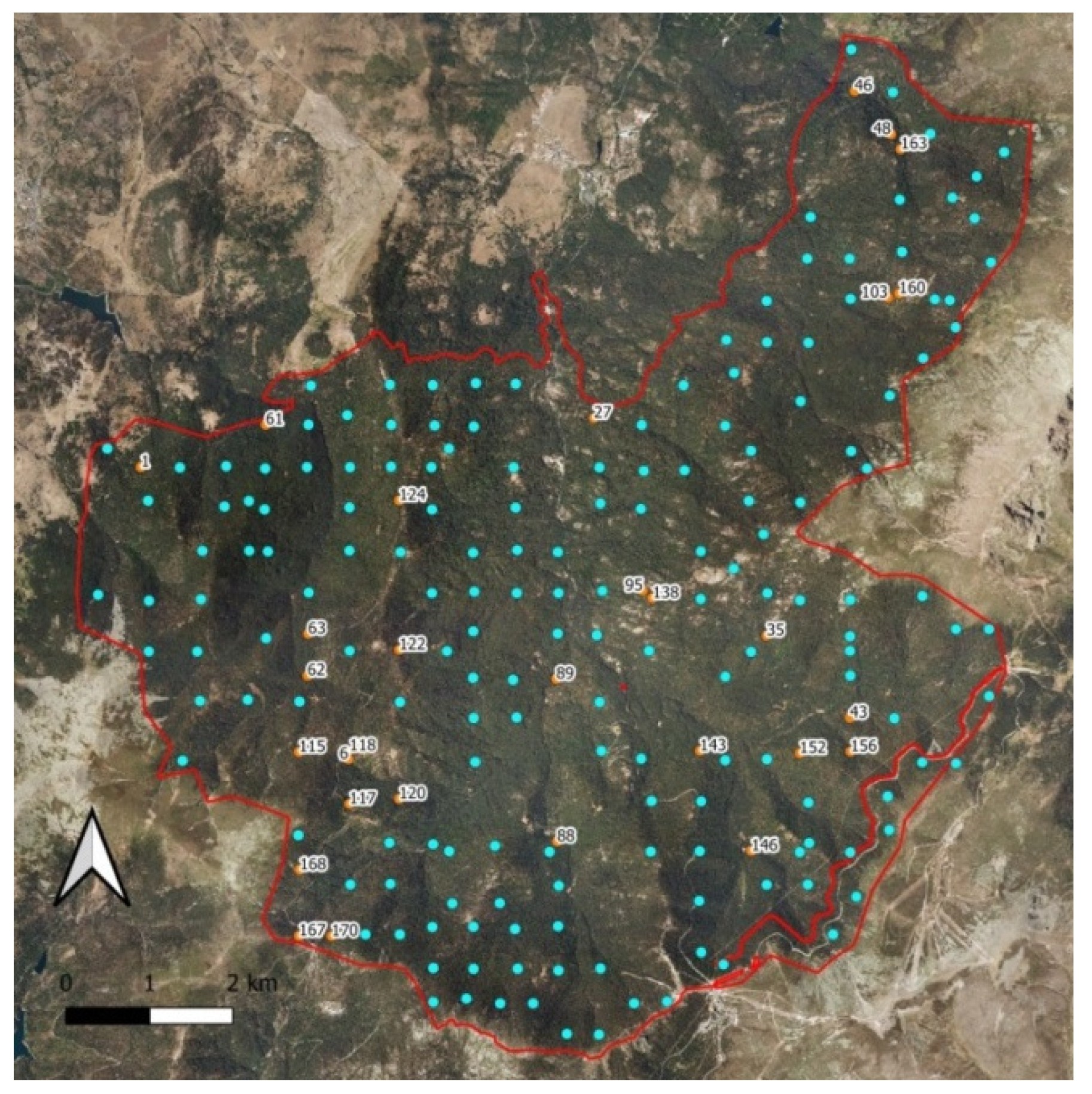
2.1. Study Area and Field Data

The study area is located in Pinar de Valsaín at Sierra de Guadarrama National Park, in Segovia province (40°51′ N, 04°01′ W). The area covers 7448 ha of a mountain public forest dominated by Scots pine (Pinus sylvestris L.) with traditional forest management activities for high-quality timber production since the 19th century. The stand includes a variety of forest structure resulting from even-aged forest management based on natural regeneration in a wide range of altitude (1260–1995 m). Topography is characterized by rugged terrain with steep slopes (>30%) in the 60% of the area. The main vegetation in the understory includes Quercus pyrenaica Willd., Ilex aquifolium L. and ferns (Pteridium aquilinum (L.) Kuhn) in the lower elevations, whereas shrubs such as Juniperus communis subsp. alpine (Suter) Čelak, Cytisus oromediterraneus Rivas Mart. et al. and Adenocarpus hispanicus (Lam.) DC. are commonly found at higher elevations. Annual precipitation ranges from 720 to 1320 mm depending on elevation, with snow often present in winter. Mean minimum and maximum temperature are −1 °C and 22 °C in January and July, respectively. Fire season corresponds to summer, with the firefighting services generally activated in the study area from 1st July to 30th September.
A forest field inventory was performed during fall–winter 2009/2010 including 202 circular plots (radius = 13 m), where diameter at breast height (DBH) was measured at two perpendicular directions for all trees with DBH ≥ 7.5 cm using a graduated caliper. Tree heights were measured with a Vertex hypsometer for the three dominants trees in each plot. In fall-winter 2016/2017, a subset of 30 circular plots (radius = 14.1 m) from the existing systematic sampling in the previous forest inventory were re-measured for detailed forest fuel characterization (Figure 1). In addition to all DBH ≥ 7.5 cm, additional measures of tree height and live crown base height (i.e., the lowest insertion point of live branches in the crown, excluding isolated branches, as defined in previous studies [4,5]) were taken in 10 randomly selected trees per plot. Trees included at 13 and 14.1 m radius were registered in the second forest inventory to compare field data and LiDAR metrics extracted from both sample sizes. Plot locations were recorded with a hand-held GNSS GPS receiver (Trimble Geo 7x unit) providing submeter accuracy after post-processing in both field inventories (2009/2010 and 2016/2017) required for accurate LiDAR point cloud matching. Post-processing was performed with Trimble GPS Pathfinder Office software using the Base Station Network from the Spanish National Geographic Institute (IGN), applying differential corrections to the raw GPS receiver files that resulted in an average horizontal accuracy of 0.225 m.
Tree height data were used to calculate stand height (H) and CBH (m) at plot level. H and CBH were calculated as the average value of total heights and live crown base heights, respectively, measured at tree level in each plot. Available CFL (kg/m2) may include foliage and small branches (diameter < 6 mm), although needles are generally considered the main aerial fuel consumed within the flaming front of a crown fire in conifer stands [17,25]. Previous allometry for the same pine species provided biomass estimations of either foliar or branches < 20 mm based on equations using DBH as the input variable [38]. Hence, CFL at plot level in this study was considered as foliar biomass, aggregating tree-level calculations of needle biomass obtained from the available allometric equations for the species. Assuming a homogeneous fuel distribution in the canopy, CBD (kg/m3) at plot level was retrieved from CLF (kg/m2) and average canopy length in each plot calculated as the difference between H and CBH (m). This approach was also used in previous studies [4,5] as it is consistent with the criteria for crown fire initiation and spread proposed by Van Wagner [16] and integrated in most fire simulation models [27].

2.2. ALS Data

Airborne LiDAR information used corresponded to four acquisition flights performed in the study area at different pulse density (Table 1). Lower point clouds corresponding to the first and second PNOA coverage were obtained in LAZ format from the CNIG website (Centro Nacional de Información Geográfica) of the Spanish National Geographic Institute (IGN). Higher point clouds were acquired by SPASA in a specific flight planned for this study and provided in LAZ format by the company. Two datasets from PNOA 2nd coverage were available due to overlapping areas between contiguous provinces (Segovia and Madrid). Pulse density was planned initially to be the same in PNOA-2016 and PNOA-2018 (1 p/m2) but was finally performed with higher density in the overlapping area, registering an average of 1.7 p/m2 in the field plots.
LiDAR data processing was performed in FUSION [39] and QGIS [40]. Return heights from the point clouds were classified to discriminate vegetation from soil. Soil returns were used to generate a digital terrain model (DTM) at 2 m resolution that was used to normalized vegetation return heights.
A set of LiDAR metrics directly obtained from FUSION software were extracted at the field plots from normalized vegetation returns (Table 2). Statistics were obtained with a threshold level of 2 m to avoid including returns not corresponding to tree crowns. The percentage of returns normalized by height strata (PRN_Si) were also calculated, based on vegetation returns within and below each layer (see equation in Table 2) as proposed by [41], to better account for laser attenuation through the canopy with different point densities [42]. PRN_Si were obtained for different strata intervals including higher detail in lower heights, with 1-m strata up to 16 m and 2-m strata above 16 m. Previous studies assessing vertical profile from LiDAR returns also used more detailed strata in the lower heights [30,43].

2.3. Statistical Analysis and Modelling

Parametric regression analysis was used to estimate CBH, CFL and CBD from LiDAR metrics derived from PNOA-2018 point clouds, using field plots from the 2016/2017 inventory as reference data. Three different model formulations were tested: linear (Equation (1)), power (Equation (2)) and exponential (Equation (3)).
Y = a 0 + a 1 X 1 + a 2 X 2 + + a j X j + ε
Y = a 0   X 1 a 1   X 2 a 2     X j a j + ε
Y = e a 0   e a 1 X 1   e a 2 X 2     e a j X j   + ε
where Y is the canopy fuel attribute to be modelled (CBH, CFL or CBD), Xj are the LiDAR metrics included as predictors and aj are the coefficients of each parameter in the model fitted, with a0 accounting for the independent term, and ε is the additive error term assumed to be normally distributed in Equation (1). To solve model fitting in non-linear formulation, logarithmic transformations were applied to power and exponential forms, resulting in Equations (4) and (5), respectively:
L n ( Y ) = L n ( a 0 ) + a 1 L n ( X 1 ) + a 2 L n ( X 2 ) + + a j L n ( X j )
L n ( Y ) = L n ( a 0 ) + a 1 X 1 + a 2 X 2 + + a j X j
Histograms and Shapiro–Wilk test were used to check normality distribution in the dependent variables (CBH, CFL and CBD) prior to parametric model fitting. Different combinations of metrics were tested, selecting the best models for each canopy fuel property and formulation type according to the significance level (p-value < 0.05) of every input parameter and the overall model performance. Adjusted R2 was used to consider the effect of varying sampling size in the different datasets. Error level was calculated as both the root mean square error (RMSE) and the mean absolute percentage error (MAPE), the latter used to facilitate comparison of model estimations among canopy fuel properties with different units.
Pearson correlation matrix was obtained for each dataset prior to model fitting to identify relevant LiDAR metrics and potential correlation between variables. In addition, multicollinearity was checked in input metrics included as predictors in multivariate models (variance inflation factor, VIF < 5). Linear regression model assumptions were also checked, including homocedasticity, normality and independence of residuals. All statistical analyses were performed with R software [44].

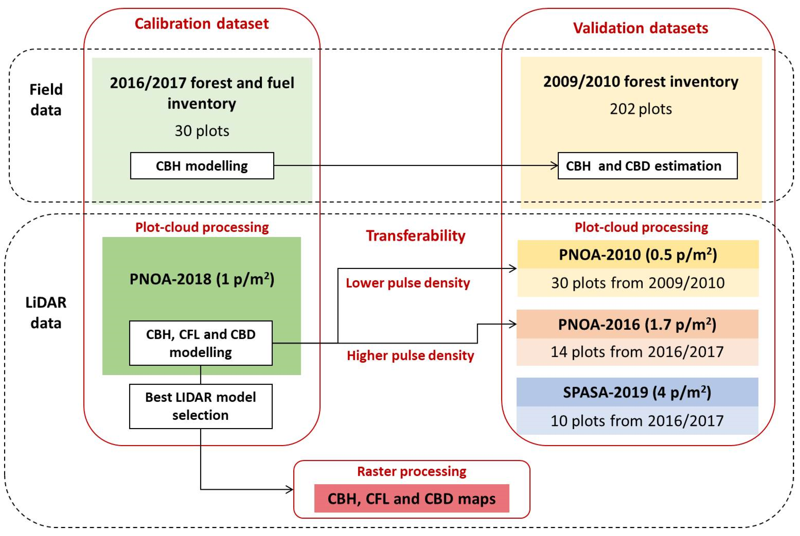
2.4. Transferibility Assessment and Canopy Fuel Mapping

Transferability assessment to higher pulse density was performed applying the models previously fitted with the calibration dataset, i.e., metrics derived from PNOA-2018 used as predictors, to the rest of available LiDAR point clouds in the study area (Table 1). Field data from the 2016/2017 inventory was used as reference of canopy fuel values. This method allowed for an independent validation of model transferability to LiDAR data acquired in 14 and 10 plots, respectively, with an increase of pulse density of 70% (PNOA-2016) and 400% (SPASA). Date and location of forest treatments performed in the study area during the 2016–2019 period were checked to ensure that any disturbance occurred in the field plots before LiDAR flights. Similarly to a previous study by [28], the three-year time lag between LiDAR data and field inventory was considered negligible for forest stand characterization. Hence, the assessment of model transferability to PNOA-2016 and SPASA datasets was addressed taking into account the effect of return density in quasi-simultaneous LiDAR data acquisitions.
CBH, CFL and CBD were obtained for each LiDAR dataset and model formulation (linear, power and exponential). Model transferability was assessed by the R2, RMSE, MAPE and bias from observed and predicted values. A correction factor (CF) based on residual standard error (RSE) of the fitted models was considered in the estimation of fuel properties with power and exponential formulation, adding the following CF term (Equation (6)) to the predicted values to account for the underestimation bias resulting from logarithmic transformation in Equations (4) and (5):
C F = e ( R S E 2 2 )
To address model transferability to lower LiDAR pulse density, metrics from PNOA-2010 were used as input data considering field data from the first forest inventory (2009/2010) as reference data. CFL was calculated in the same 30 plots that were re-measured in the 2016/2017 forest inventory following the same methods described in Section 2.1. However, CBH and CBD could not be derived from available field data. A regression model was first fitted to estimate CBH at plot level from H values from 2016/2017 forest inventory that was applied to 2009/2010 field data. CBD was then calculated as described in Section 2.1. Regarding LiDAR data, metrics were also extracted at 13 m radius to get point-cloud statistics equivalent to the smaller field sampling size in the first forest inventory.
Finally, the best models resulting from the previous modelling and transferability assessment were selected to generate maps for each canopy fuel attribute at 25 m resolution (equivalent to the 14.1 m radius size used in the calibration dataset) from LiDAR metrics obtained in raster format for the whole study area. MDT previously generated (Section 2.2) was used to normalize returns prior to metric extraction in 25 m cells. A schematic diagram of the study work-flow is shown in Figure 2.

3. Results

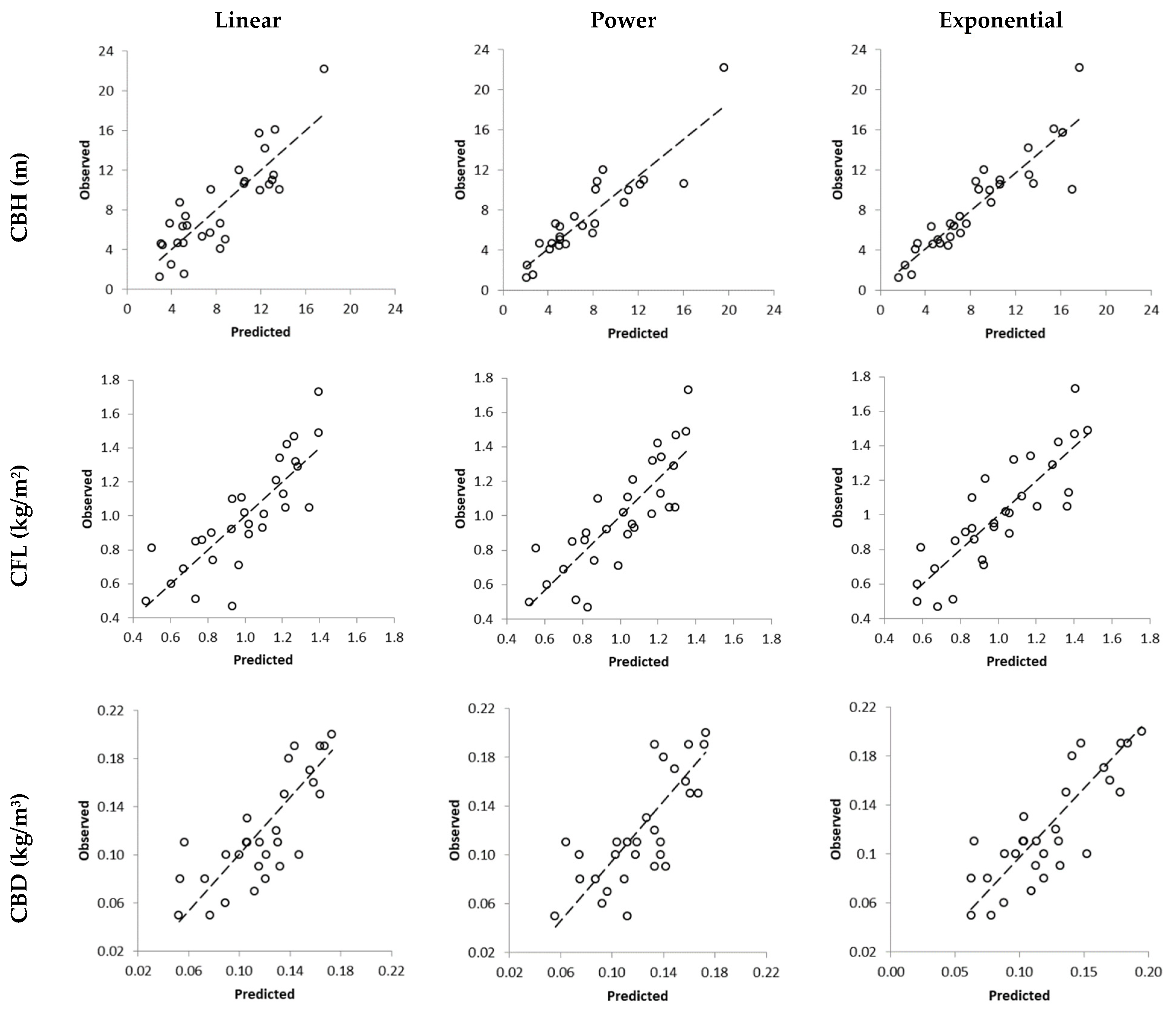
3.1. Canopy Fuel Modelling

Detailed field data for canopy fuel characterization obtained in the 30 re-measured plots during the 2016/2017 forest inventory (Table 3) was used to calibrate models for CBH, CFL and CBH estimation from PNOA-2018 LiDAR metrics. Table 4 summarizes results for the best models found for each dependent variable and formulation. In general, exponential models had the best performance for the three canopy fuel attributes. Observed versus predicted values are shown in Figure 3.
CBH was the canopy fuel variable showing the strongest relationship with LiDAR metrics, independently of the regression method used. Variability explained by the CBH models (R2adj) ranged from 0.70 to 0.87, with RMSE between 1.8 and 2.4 m and MAPE ranging 18% to 38%. Selected input metrics in the best models were the same for the power and exponential formulation, and in all cases a PRN metric accounting for return density in low height strata was included (6–8 m in the linear model, 3–4 m in power and exponential models).
CFL models showed more moderate results compared to CBH models in terms of R2adj (0.62–0.68) but had better levels of estimation error, with RMSE of 0.17–0.18 kg/m2 and MAPE of 14–16%. PFR was a predictor metric in all model formulations, showing the best results either combined with a low percentile (P05 in the power function) or PRN in low height strata.
CBD models showed the worse fitting results to LiDAR metrics, with similar R2adj of 0.58 for linear and exponential formulations that performed significantly better than the power model (0.47). Error levels were intermediate to observed values in CBH and CFL models, with RMSE ranging 0.03–0.04 kg/m3 and MAPE of 20–22%. Regarding input metrics, all models included PFR as in CLF models, but in this case only linear and exponential formulations showed better results adding PRN in low height strata.

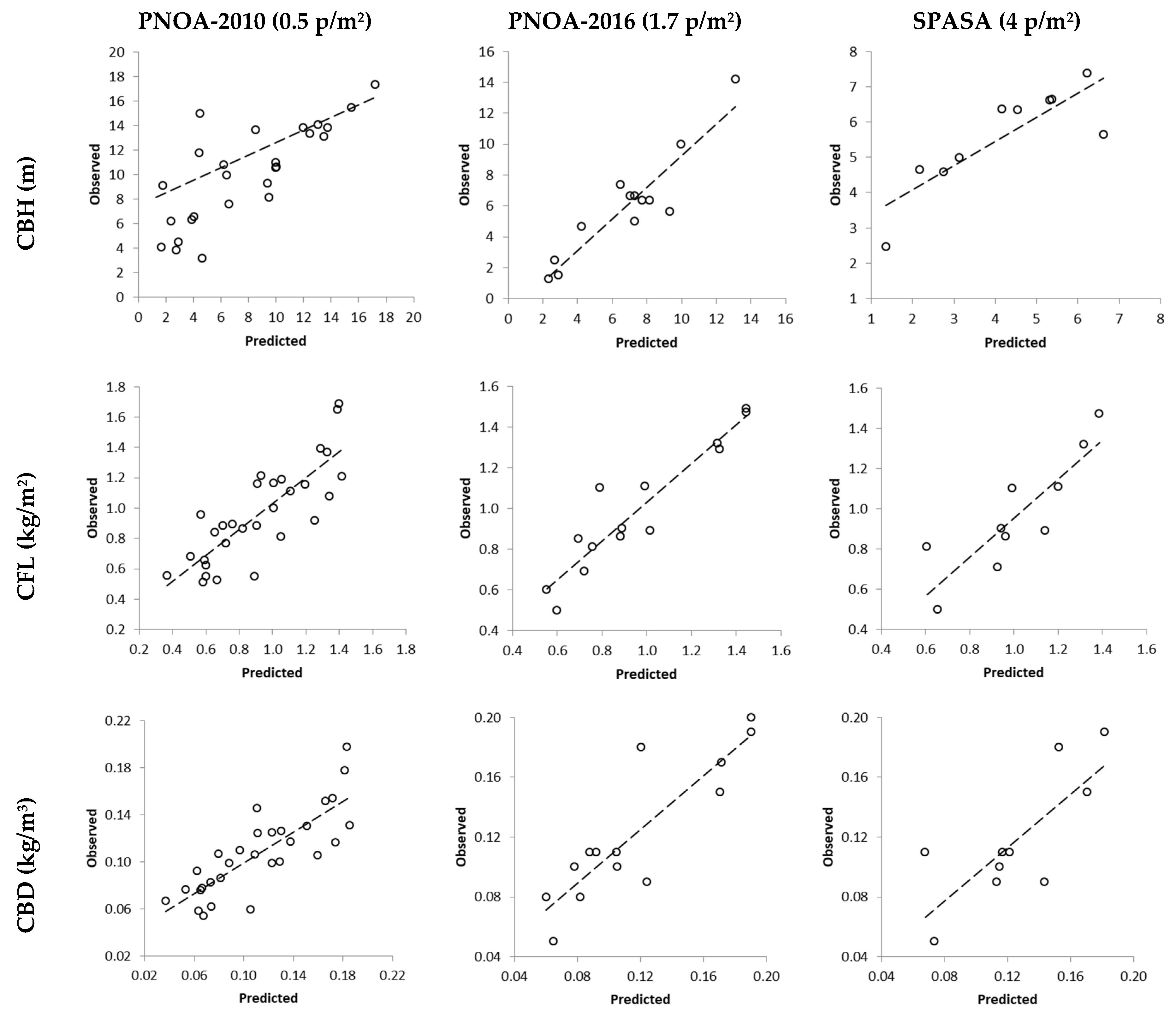
3.2. Transferability Assessment

A regression model was fitted with field data from 2016/2017 forest inventory to estimate CBH field values that could not be directly retrieved from 2009/2010 forest inventory. Equation (7) shows the best model found that provides CBH estimates in the field plots from H values (R2= 0.91, p < 0.00001, RMSE = 1.4 m y MAPE = 15.9%):
CBH = 6.661823 + 0.8841 × H
Once CBH was calculated, CBD at plot level could be also retrieved with the same method used for the 2016/2017 forest inventory (as described in Section 2.1 and Section 2.3). Table 5 summarizes the stand and canopy fuel attributes in the 2009/2010 forest inventory. Similar average values were observed for CFL and CBD, with slightly higher minimum and mean CBH values. Previous statistical analyses reported that there were no significant differences in stand and canopy fuel variables between both forest inventories despite the 7-year time lag in the field datasets [42].
The best fitted models obtained for each canopy fuel variable and formulation (Table 4) were applied to the three other LiDAR datasets available in the study area (Table 1). Model extrapolation resulted in different transferability level depending on pulse density (higher and lower LiDAR returns), type of formulation (linear, power and exponential) and canopy fuel variable (Table 6).
The transferred CBH model resulted in the higher variability of performance and error level, with R2 between observed and predicted values ranging from 0.08 to 0.87, RMSE from 1.4 to 6.9 m, MAPE from 20% to 47% and bias from −1.4 to 4.8 m. Model performance significantly varied depending on the LiDAR dataset and model formulation, with the highest bias in model transfer to the lower pulse density (PNOA-2010).
Transferability assessment for CFL and CBD showed a more consistent model performance between LiDAR datasets. The transferred CFL model resulted in R2 between observed and predicted values from 0.66 to 0.89 with RMSE, MAPE and bias levels ranging 0.11–0.19 kg/m2, 9–18% and −0.05–0.11 kg/m2, respectively, and the best performance in the PNOA-2016 dataset for all formulation methods.
R2 values in transferred CBD models were lower compared to CFL ranging from 0.51 to 0.77. Error level was more homogeneous in terms of RMSE of 0.022–0.029 kg/m3, whereas MAPE ranged 14% to 31% and bias from −0.016 to 0.013 kg/m3. Similar to CFL, the PNOA-2016 dataset showed the best performance for all formulation methods.
Regarding the different LiDAR datasets, all canopy fuel variables showed the best model transfer performance with PNOA-2016 which had a slightly higher pulse density (1.7 p/m2) compared to the PNOA-2018 dataset (1 p/m2) used for calibration. These results were consistent independent of model formulation, thus confirming the effect of return density on model transferability. The extrapolation of CBH models to the PNOA-2016 dataset reported the worse performance in the linear model (R2 = 0.52 y MAPE = 47%), with good level of correlation in power and exponential formulations between observed and predicted values (R2 from 0.85 to 0.87) but high error level (MAPE from 30% to 36%). Transferred CFL model performance in this LiDAR dataset was similar in all formulations with good accuracy (R2 from 0.88 to 0.89, MAPE from 8% to 13%). Extrapolation of the CBD model also resulted in adequate performance for all formulations in this pulse density (R2 from 0.76 to 0.77, MAPE from 14% to 16%).
With regard to the transferability assessment in the higher density LiDAR dataset (SPASA, 4 p/m2), the exponential models showed a significant higher performance for all canopy fuel attributes. Best results between observed and predicted values were found for the extrapolation of the CFL model (R2 = 0.74, MAPE = 15%), followed by CBH model (R2 = 0.72 y MAPE = 31%) and CBD model (R2 = 0.60 y MAPE = 23%).
Model transfer to the lower density LiDAR dataset (PNOA-2010, 0.5 p/m2) resulted in very low performance for CBH estimation in all formulations (R2 < 0.28 y MAPE > 32%). However, transferability of CFL and CBD model showed better results, with a similar or even a better performance compared to model transfer to the higher pulse density (4 p/m2). CFL showed the best results for power formulation (R2 = 0.67 y MAPE = 15%) whereas the exponential formulation had the best transferability level in the CBD models (R2 = 0.68 y MAPE = 21%).
Overall, exponential models showed a better performance, though differences were observed between canopy fuel variables (CBH, CFL, and CDB). Figure 4 represents observed versus predicted values for exponential models transferred to each LiDAR dataset.

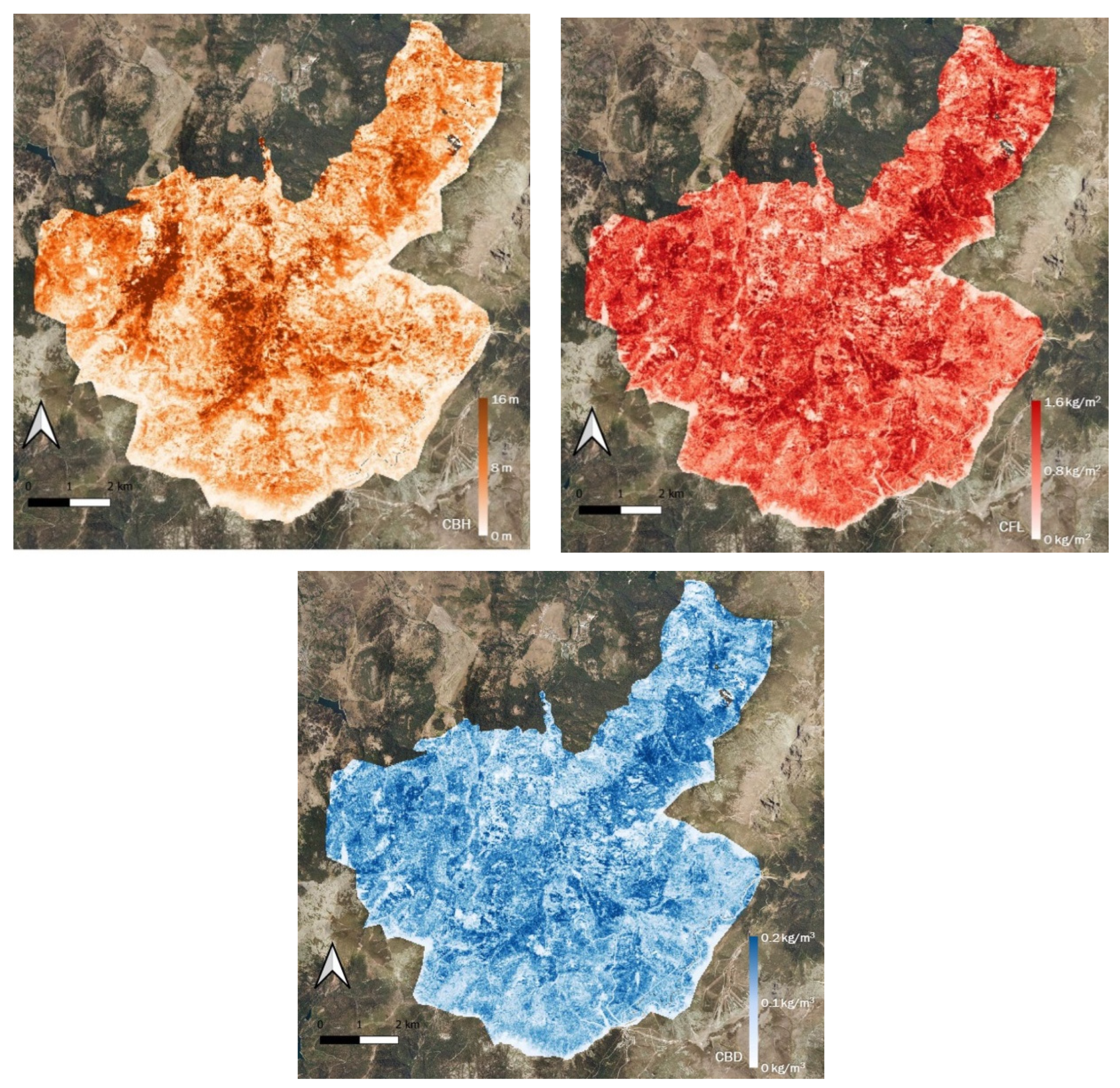
3.3. Canopy Fuel Mapping

According to the previous results, the exponential models were selected to generate wall-to-wall canopy fuel products over the whole area. LiDAR data from PNOA-2018 were processed to obtain raster layers of metrics required as input in each model (CBH, CFL, CBD). Resulting high resolution fuel maps (25 × 25 m) generated for the study area are shown in Figure 5, providing spatially-explicit information of canopy fuels for fire behavior simulations. High CBH values were generally found in lower altitudinal ranges corresponding to mature stands located in high quality sites, whereas low CBH values were located in very high altitudes (i.e., south and east limits of the study area, corresponding to low quality sites) or younger stands (regeneration patches). As expected, we found a similar pattern of CFL and CBD spatial variability distribution, which were highly dependent on forest canopy cover (i.e., PFR metric) in accordance with model formulation.

4. Discussion

This study confirms that low-density LiDAR data (1 p/m2) acquired from aerial platforms to provide large-scale coverage at regional level can be effectively used to retrieve models to estimate canopy fuel variables that are critical for fire behavior simulation. Regression analysis indicated the best fitting model was found for CBH, followed by CFL, with CBD being the canopy fuel variable more difficult to estimate. Our results in a natural pure pine stand (Pinus sylvestris L.) are in agreement with previous findings using very low pulse density (0.5 p/m2) in other conifer or mixed stands from temperate and Mediterranean forest areas [4,27,37,45,46]. However, our study showed significantly better results compared to previous regression models derived from low-density LiDAR for the same pine species [46]. With higher return density, some authors reported similar or higher accuracy for CFL and CBD estimation compared to CBH [26,47] or higher for CFL compared to CBH and CBD [28] in mixed or pure conifer forest stands.
Transferability assessment of the best fitted regression models for each type of formulation to three different point cloud datasets in the same study area indicated varying level of accuracy, depending on LiDAR pulse density (both higher and lower than the calibration dataset) and model formulation (linear, power and exponential). Differences were also observed regarding the canopy fuel attribute (CBH, CFL and CBD).
The best results were generally found for exponential models in all canopy fuel variables, both in the calibration phase with the 1 p/m2 LiDAR dataset and in the extrapolation for model validation in independent LiDAR flights acquired in the same study area with either lower (0.5 p/m2) or higher pulse density (1.7 and 4 p/m2). Linear models have been traditionally among the most commonly used method in parametric regression modelling to predict canopy fuels from airborne LiDAR metrics [4,26,27]. However, our results highlight that direct transfer of this kind of models for canopy fuel mapping may result in higher bias errors compared to other parametric regression forms, suggesting exponential formulation as an alternative for model fitting with calibration datasets.
For all canopy fuel variables addressed in this study, our results indicated a better model performance when transferred to a pulse density of 1.7 p/m2 compared to 0.5 and 4 p/m2, independently of the model formulation used. These findings highlight the effect of LiDAR pulse density on canopy fuel model transferability, indicating that significantly different results in accuracy could be found in direct extrapolation of previous models to LiDAR datasets acquired with different conditions than the one used for model calibration, even for relatively similar low pulse densities.
For example, positive bias (overestimation) was observed for CBH in the lower (0.5 p/m2) and higher (4 p/m2) pulse density, whereas a negative bias (underestimation) resulted in the intermediate pulse density (1.7 p/m2) independent of model formulation. This are relevant result when applying models to map canopy fuels to be used in simulation tools, as CBH overestimation may lead to unrealistic lower perception of crown fire potential in forest stands. From a conservative point of view, fire prevention and management actions based on simulation may benefit from fuel maps with CBH underestimation. Similarly, for all model formulations CFL estimation showed positive bias (overestimation) for the extrapolation to 0.5 and 1.7 p/m2, whereas a negative bias (underestimation) was observed when models were applied to higher pulse density (4 p/m2). Conversely, CBD model showed positive (overestimation) or negative (underestimation) bias for linear or power and exponential formulations, respectively, when transferred to the lower pulse density (0.5 p/m2). In the case of higher pulse density, bias was either negative (underestimation) for 1.7 p/m2 or positive (overestimation) for 4 p/m2 independently of model formulation. In this sense, Mauro et al. [28] found a consistent overestimation in CBH, CFL and CBD in parametric model transfer to pulse densities higher that the ones included in our study (>8 p/m2). These authors reported better results in model transferability in semiparametric models compared to parametric models, highlighting that calibration could substantially reduce bias in the latter.
Despite the fact that CBH was the canopy fuel variable showing a stronger correlation with LiDAR metrics in the calibration phase, error levels were higher compared to CFL and CBD. Exponential formulation considerably reduced RMSE and MAPE compared to the linear model. Transferability assessment indicated that the worse CBH model performance was observed for the lower pulse density LiDAR dataset (0.5 p/m2). This finding may be taken with caution as a propagation error due to CBH estimation in the 2009/2010 forest inventory, where field data to directly retrieve this canopy attribute were unavailable, may be affecting the results. Another potential explanation for the worse performance in CBH model transfer to the PNOA-2010 LiDAR dataset could be due to the lower penetration capacity of a laser pulse with 0.5 p/m2 compared to higher pulse densities, being unable to get sufficient returns from the lower part of the canopy [30]. This effect may be more patent in the metrics used in the CBH model where inputs in the calibration model combined return statistics (mean, skew) and lower strata return density (PRN_3-4), compared to CFL and CBD models where inputs included percentage of first returns (PFR) suggesting that this density metric may be less affected by laser attenuation in our LiDAR datasets. In a previous study, Navarro et al. [35] highlighted the relevance of selecting stable metrics to improve model transferability to different LiDAR data. Further research is required to analyze the pulse density effect on different LiDAR metrics.
Exponential models fitted to estimate canopy fuel attributes with PNOA-2018 dataset (1 p/m2) were used to generate high resolution maps (25 m pixel) of CBH, CFL and CBD over the entire study area. These products increased reliability of previous cartography in the area of interest, providing valuable spatial information to be used in fire behavior simulation models to assess potential crown fire risk and severity in the forest stand and support fuel treatment planning [1,2].
Further work is required to verify that exponential formulation provides more robust results in terms of regression model transferability for canopy fuel mapping in other forest species and LiDAR datasets (pulse density > 4 p/m2). More research is also needed to test non-parametric model transferability to validate our results regarding the effect of pulse density with machine learning techniques that are increasingly used to retrieve forest stand and fuel attributes from LiDAR metrics [28,35,48]. Domingo et al. [34] found better transferability with non-parametric regression to estimate different forest stand attributes. However, the flexibility of these non-parametric methods, that impose no structure in the model errors, makes it difficult to calibrate pre-existing models to new data collections [28]. Navarro et al. [35] suggested a new variable selection method to use stable metrics which enhanced the transfer capacity of Support Vector Regression (SVR) models, demonstrating that SVR models using stable metrics can be transferred not only to point clouds acquired using the same technology (i.e., airborne LiDAR) but also between different technologies (e.g., data from digital aerial photogrammetry) without a significant loss of accuracy to estimate growing stock volume in forest stands. Future work may focus on testing these methods in canopy fuel attributes. Mauro et al. [28] also suggest the use of semiparametric models that combine flexibility in modelling nonlinear patterns of the non-parametric methods with parametric assumptions about the structure of the model errors with the possibility of calibrating predictions.

5. Conclusions

This study provides new models to estimate canopy base height, fuel load and bulk density in pure Pinus sylvestris stands with low density LiDAR data. A transferability assessment to three different LiDAR flights (0.5, 1.7 and 4 p/m2) acquired over the same study area was also conducted. Our results highlight that direct transfer of parametric regression models derived from airborne LiDAR data to generate canopy fuel maps may result in significant bias error. Caution should be taken when extrapolating models to new LiDAR datasets with different pulse density. Type of formulation may be also carefully considered in calibration studies to increase model transferability for critical canopy fuel attribute estimation with future LiDAR acquisition datasets.

Author Contributions

Conceptualization, E.M., J.L.T., J.M., M.G. and C.H.; methodology, E.M. and J.L.T.; software, E.M. and J.L.T.; validation, E.M.; formal analysis, E.M.; investigation, E.M.; writing—original draft preparation, E.M.; visualization, E.M.; supervision, E.M., J.L.T. and J.M.; project administration, E.M., J.L.T. and J.M.; funding acquisition, E.M., J.L.T., J.M., M.G. and C.H. All authors have read and agreed to the published version of the manuscript.

Funding

This research was partially funded by the Spanish National Research Institute for Agriculture (INIA) through projects VIS4FIRE (RTA2017-00042-C05-01) and GEPRIF (RTA2014-00011-C06-06), and co-funded by the EU-FEDER program. Eva Marino’s participation was also partially funded by a postdoctoral grant from the Spanish Ministry of Economy and Competitiveness (Torres-Quevedo program) supported by the European Social Fund (ESF).

Institutional Review Board Statement

Not applicable.

Informed Consent Statement

Not applicable.

Data Availability Statement

Not applicable.

Acknowledgments

The authors thank Centro de Montes y Aserradero de Valsaín from Organismo Autónomo Parques Nactionales for providing 2009/2010 forest inventory and ancillary data of the study area. We acknowledge Servicios Politécnicos Aéreos, S.A. (SPASA) for providing LiDAR data from the 2019 flight. We are also grateful to our colleagues from INIA and AGRESTA that help during the 2016/2017 field inventory, and P. Ascasibar for his help with GPS data postprocessing.

Conflicts of Interest

The authors declare no conflict of interest.

References

  1. Alcasena, F.J.; Salis, M.; Ager, A.A.; Arca, B.; Molina-Terren, D.; Spano, D. Assessing Landscape Scale Wildfire Exposure for Highly Valued Resources in a Mediterranean Area. Environ. Manag. 2015, 55, 1200–1216. [Google Scholar] [CrossRef] [PubMed]
  2. Salis, M.; Laconi, M.; Ager, A.A.; Alcasena, F.J.; Arca, B.; Lozano, O.; Fernandes de Oliveira, A.; Spano, D. Evaluating alternative fuel treatment strategies to reduce wildfire losses in a Mediterranean area. For. Ecol. Manag. 2016, 368, 207–221. [Google Scholar] [CrossRef]
  3. Cardil, A.; Monedero, S.; Schag, G.; de-Miguel, S.; Tapia, M.; Stoof, C.R.; Silva, C.A.; Mohan, M.; Cardil, A.; Ramírez, J. Fire behavior modeling for operational decision-making. Curr. Opin. Environ. Sci. Health 2021, 23, 100291. [Google Scholar] [CrossRef]
  4. Botequim, B.; Fernandes, P.M.; Borges, J.G.; González-Ferreiro, E.; Guerra-Hernández, J. Improving silvicultural practices for Mediterranean forests through fire behaviour modelling using LiDAR-derived canopy fuel characteristics. Int. J. Wildland Fire 2019, 28, 823–839. [Google Scholar] [CrossRef]
  5. Arellano-Pérez, S.; Castedo-Dorado, F.; Álvarez-González, J.G.; Alonso-Rego, C.; Vega, J.A.; Ruiz-González, A.D. Mid-term effects of a thin-only treatment on fuel complex, potential fire behaviour and severity and post-fire soil erosion protection in fast-growing pine plantations. For. Ecol. Manag. 2020, 460, 117895. [Google Scholar] [CrossRef]
  6. Finney, M.A. FARSITE: Fire Area Simulator—Model Development and Evaluation; RMRS-RP-4; USDA Forest Service: Washington, DC, USA, 1998.
  7. Finney, M.A. An Overview of FlamMap Modeling Capabilities; Research Paper RMRS-P-41; USDA Forest Service: Washington, DC, USA; Rocky Mountain Research Station: Fort Collins, CO, USA, 2006.
  8. Alexander, M.E.; Cruz, M.G. Limitations on the accuracy of model predictions of wildland fire behaviour: A state-of-the-knowledge overview. For. Chron. 2013, 89, 372–383. [Google Scholar] [CrossRef]
  9. IPCC. Climate Change 2021: The physical science basis. In Contribution of Working Group I to the Sixth Assessment Report of the Intergovernmental Panel on Climate Change; IPCC: Genva, Switzerland, 2021. [Google Scholar]
  10. Abram, N.J.; Henley, B.J.; Gupta, A.S.; Lippmann, T.J.R.; Clarke, H.; Dowdy, A.J.; Sharples, J.J.; Nolan, R.H.; Zhang, T.; Wooster, M.J.; et al. Connections of climate change and variability to large and extreme forest fires in southeast Australia. Commun. Earth Environ. 2021, 2, 8. [Google Scholar] [CrossRef]
  11. Moreira, F.; Ascoli, D.; Safford, H.; Adams, A.M.; Moreno, J.M.; Pereira, J.C.; Catry, F.X.; Armesto, J.; Bond, W.J.; E González, M.; et al. Wildfire management in Mediterranean-type regions: Paradigm change needed. Environ. Res. Lett. 2020, 15, 011001. [Google Scholar] [CrossRef]
  12. Goss, M.; Swain, D.L.; Abatzoglou, J.T.; Sarhadi, A.; A Kolden, C.; Williams, A.P.; Diffenbaugh, N.S. Climate change is increasing the likelihood of extreme autumn wildfire conditions across California. Environ. Res. Lett. 2020, 15, 094016. [Google Scholar] [CrossRef]
  13. Nolan, R.H.; Boer, M.M.; Collins, L.; Resco de Dios, V.; Clarke, H.G.; Jenkins, M.; Kenny, B.; Bradstock, R.A. Causes and consequences of eastern Australia’s 2019–2020 season of mega-fires. Glob. Chang. Biol. 2020, 26, 1039–1041. [Google Scholar] [CrossRef] [Green Version]
  14. Williams, A.P.; Abatzoglou, J.T.; Gershunov, A.; Guzman-Morales, J.; Bishop, D.A.; Balch, J.K.; Lettenmaier, D.P. Observed Impacts of Anthropogenic Climate Change on Wildfire in California. Earth’s Futur. 2019, 7, 892–910. [Google Scholar] [CrossRef]
  15. Wotton, B.M.; Flannigan, M.D.; Marshall, G.A. Potential climate change impacts on fire intensity and key wildfire suppression thresholds in Canada. Environ. Res. Lett. 2017, 12, 95003. [Google Scholar] [CrossRef]
  16. Van Wagner, C.E. Conditions for the start and spread of crown fire. Can. J. For. Res. 1977, 7, 23–34. [Google Scholar] [CrossRef]
  17. Cruz, M.G.; Alexander, M.E.; Wakimoto, R.H. Assessing canopy fuel stratum characteristics in crown fire prone fuel types of western North America. Int. J. Wildland Fire 2003, 12, 39–50. [Google Scholar] [CrossRef]
  18. Molina, J.R.; Silva, F.R.Y.; Mérida, E.; Herrera, M. Modelling available crown fuel for Pinus pinaster Ait. stands in the “Cazorla, Segura and Las Villas Natural Park” (Spain). J. Environ. Manag. 2014, 144, 26–33. [Google Scholar] [CrossRef] [PubMed]
  19. Lefsky, M.; Cohen, W.; Acker, S.; Parker, G.; Spies, T.; Harding, D. Lidar Remote Sensing of the Canopy Structure and Biophysical Properties of Douglas-Fir Western Hemlock Forests. Remote Sens. Environ. 1999, 70, 339–361. [Google Scholar] [CrossRef]
  20. Hudak, A.T.; Crookston, N.L.; Evans, J.S.; Hall, D.E.; Falkowski, M.J. Nearest neighbor imputation of species-level, plot-scale forest structure attributes from LiDAR data. Remote Sens. Environ. 2008, 112, 2232–2245. [Google Scholar] [CrossRef]
  21. Maltamo, M.; Næsset, E.; Vauhkonen, J. Forestry Applications of Airborne Laser Scanning: Concepts and Case Studies. In Managing Forest Ecosystems; Springer: Brlin/Heidelberg, Germany, 2014. [Google Scholar]
  22. Marino, E.; Ranz, P.; Tomé, J.L.; Noriega, M.A.; Esteban, J.; Madrigal, J. Generation of high-resolution fuel maps from discrete airborne laser scanner data and Landsat-8 OLI: A low-cost and highly updated methodology for large areas. Remote Sens. Environ. 2016, 187, 267–280. [Google Scholar] [CrossRef]
  23. García, M.; Riaño, D.; Chuvieco, E.; Salas, J.; Danson, F. Multispectral and LiDAR data fusion for fuel type mapping using Support Vector Machine and decision rules. Remote Sens. Environ. 2011, 115, 1369–1379. [Google Scholar] [CrossRef]
  24. Huesca, M.; Riaño, D.; Ustin, S.L. Spectral mapping methods applied to LiDAR data: Application to fuel type mapping. Int. J. Appl. Earth Obs. Geoinf. ITC J. 2019, 74, 159–168. [Google Scholar] [CrossRef] [Green Version]
  25. Riaño, D.; Meier, E.; Allgöwer, B.; Chuvieco, E.; Ustin, S.L. Modeling airborne laser scanning data for the spatial generation of critical forest parameters in fire behavior modeling. Remote Sens. Environ. 2003, 86, 177–186. [Google Scholar] [CrossRef]
  26. Andersen, H.-E.; McGaughey, R.J.; Reutebuch, S.E. Estimating forest canopy fuel parameters using LIDAR data. Remote Sens. Environ. 2005, 94, 441–449. [Google Scholar] [CrossRef]
  27. Gonzalez-Ferreiro, E.; Arellano-Pérez, S.; Castedo-Dorado, F.; Hevia, A.; Vega, J.A.; Vega-Nieva, D.J.; Álvarez-González, J.G.; Ruiz-González, A.D. Modelling the vertical distribution of canopy fuel load using national forest inventory and low-density airbone laser scanning data. PLoS ONE 2017, 12, e0176114. [Google Scholar] [CrossRef]
  28. Mauro, F.; Hudak, A.T.; Fekety, P.A.; Frank, B.; Temesgen, H.; Bell, D.M.; Gregory, M.J.; McCarley, T.R. Regional Modeling of Forest Fuels and Structural Attributes Using Airborne Laser Scanning Data in Oregon. Remote Sens. 2021, 13, 261. [Google Scholar] [CrossRef]
  29. González-Ferreiro, E.; Diéguez-Aranda, U.; Miranda, D. Estimation of stand variables in Pinus radiata D. Don plantations using different LiDAR pulse densities. For. Int. J. For. Res. 2012, 85, 281–292. [Google Scholar] [CrossRef]
  30. Jakubowski, M.K.; Guo, Q.; Kelly, M. Tradeoffs between lidar pulse density and forest measurement accuracy. Remote Sens. Environ. 2013, 130, 245–253. [Google Scholar] [CrossRef]
  31. Ruiz, L.A.; Hermosilla, T.; Mauro, F.; Godino, M. Analysis of the Influence of Plot Size and LiDAR Density on Forest Structure Attribute Estimates. Forests 2014, 5, 936–951. [Google Scholar] [CrossRef]
  32. Fekety, P.A.; Falkowski, M.J.; Hudak, A.T. Temporal transferability of LiDAR based imputation of forest inventory attributes. Can. J. For. Res. 2015, 45, 422–435. [Google Scholar] [CrossRef]
  33. Fekety, P.A.; Falkowski, M.J.; Hudak, A.T.; Jain, T.B.; Evans, J.S. Transferability of Lidar-derived Basal Area and Stem Density Models within a Northern Idaho Ecoregion. Can. J. Remote Sens. 2018, 44, 131–143. [Google Scholar] [CrossRef]
  34. Domingo, D.; Alonso, R.; Lamelas, M.T.; Montealegre, A.L.; Rodríguez, F.; de la Riva, J. Temporal Transferability of Pine Forest Attributes Modeling Using Low-Density Airborne Laser Scanning Data. Remote Sens. 2019, 11, 261. [Google Scholar] [CrossRef] [Green Version]
  35. Navarro, J.A.; Tomé, J.L.; Marino, E.; Guillén-Climent, M.; Fernández-Landa, A. Assessing the transferability of airborne laser scanning and digital aerial photogrammetry derived growing stock volume models. Int. J. Appl. Earth Obs. Geoinf. 2020, 91, 102135. [Google Scholar] [CrossRef]
  36. Roussel, J.-R.; Caspersen, J.; Béland, M.; Thomas, S.; Achim, A. Removing bias from LiDAR-based estimates of canopy height: Accounting for the effects of pulse density and footprint size. Remote Sens. Environ. 2017, 198, 1–16. [Google Scholar] [CrossRef]
  37. Engelstad, P.S.; Falkowski, M.; Wolter, P.; Poznanovic, A.; Johnson, P. Estimating Canopy Fuel Attributes from Low-Density LiDAR. Fire 2019, 2, 38. [Google Scholar] [CrossRef]
  38. Montero, G.; Ruiz-Peinado, R.; Múñoz, M. Producción de biomasa y fijación de CO2 por los bosques de España; INIA: Madrid, Spain, 2005; p. 270. [Google Scholar]
  39. McGaughey, R.J. FUSION/LDV: Software for LIDAR Data Analysis and Visualization, Version 3.42; U.S. Department of Agriculture, Forest Service: Washington, DC, USA; Pacific Northwest Research Station: Corvallis, OR, USA; University of Washington: Seattle, WA, USA, 2014; p. 179.
  40. QGIS Development Team; Quantum GIS Geographic Information System. Open Source Geospatial Foundation Project. 2022. Available online: http://qgis.osgeo.org/ (accessed on 22 August 2022).
  41. Skowronski, N.; Clark, K.; Nelson, R.; Hom, J.; Patterson, M. Remotely sensed measurements of forest structure and fuel loads in the Pinelands of New Jersey. Remote Sens. Environ. 2007, 108, 123–129. [Google Scholar] [CrossRef]
  42. Marino, E.; Montes, F.; Tomé, J.L.; Navarro, J.A.; Hernando, C. Vertical forest structure analysis for wildfire prevention: Comparing airborne laser scanning data and stereoscopic hemispherical images. Int. J. Appl. Earth Obs. Geoinf. 2018, 73, 438–449. [Google Scholar] [CrossRef]
  43. Kramer, H.A.; Collins, B.M.; Kelly, M.; Stephens, S.L. Quantifying Ladder Fuels: A New Approach Using LiDAR. Forests 2014, 5, 1432–1453. [Google Scholar] [CrossRef]
  44. R Development Core Team. R: A Language and Environment for Statistical Computing; R Foundation for Statistical Computing: Vienna, Austria, 2014. [Google Scholar]
  45. González-Ferreiro, E.; Diéguez-Aranda, U.; Crecente-Campo, F.; Barreiro-Fernández, L.; Miranda, D.; Dorado, F.C. Modelling canopy fuel variables for Pinus radiata D. Don in NW Spain with low-density LiDAR data. Int. J. Wildland Fire 2014, 23, 350–362. [Google Scholar] [CrossRef]
  46. Fidalgo-González, L.; Arellano-Pérez, S.; Castedo-Dorado, F.; Ruiz-González, A.D.; González-Ferreiro, E. Estimación de la distribución vertical de combustibles finos del dosel de copas en masas de Pinus sylvestris empleando datos LiDAR de baja densidad. Rev. Teledetección 2019, 53, 1–16. [Google Scholar] [CrossRef]
  47. Hevia, A.; Álvarez-González, J.G.; Ruiz-Fernández, E.; Prendes, C.; Ruiz-González, A.D.; Majada, J.; González-Ferreiro, E. Modelling canopy fuel and forest stand variables and characterizing the influence of thinning in the stand structure using airborne LiDAR. Rev. Teledetección 2016, 45, 41–55. [Google Scholar] [CrossRef]
  48. Alonso-Rego, C.; Arellano-Pérez, S.; Guerra-Hernández, J.; Molina-Valero, J.A.; Martínez-Calvo, A.; Pérez-Cruzado, C.; Castedo-Dorado, F.; González-Ferreiro, E.; Álvarez-González, J.G.; Ruiz-González, A.D. Estimating Stand and Fire-Related Surface and Canopy Fuel Variables in Pine Stands Using Low-Density Airborne and Single-Scan Terrestrial Laser Scanning Data. Remote Sens. 2021, 13, 5170. [Google Scholar] [CrossRef]
Figure 1. Plot location in the two field inventories conducted in the study area: 2009/2010 (blue) and 2016/2017 (orange, with plot identification number).
Fire 05 00126 g001
Figure 2. Conceptual diagram of the methods used for canopy fuel modelling and transferability assessment.
Fire 05 00126 g002
Figure 3. Observed vs. predicted values of canopy fuel attributes (CBH, canopy base height; CFL, canopy fuel load; CBD, canopy bulk density) resulting from model fitting with PNOA-2018 LiDAR data (n = 30) for each formulation (linear, power, exponential). Least square trend line (dashed) is shown.
Fire 05 00126 g003
Figure 4. Observed vs. predicted values of canopy fuel attributes (CBH, canopy base height; CFL, canopy fuel load; CBD, canopy bulk density) resulting from applying the best model fitted with PNOA-2018 LiDAR data (exponential) to the LiDAR datasets available in the study area with different pulse density: PNOA-2010 (n = 30), PNOA-2016 (n = 14) and SPASA (n = 10). Least square trend line (dashed) is shown.
Fire 05 00126 g004
Figure 5. Canopy fuel maps of CBH, CFL and CBD generated at 25-m pixel over the study area derived from the application of the best LiDAR model fitted for each variable (exponential formulation).
Fire 05 00126 g005
Table 1. ALS data available and corresponding field plots in the study area, including horizontal (RMSE xy) and vertical (RMSE z) accuracy. RMSE, root mean square error.
ALS DataALS FlightYearPulse DensityField PlotsRMSE xyRMSE zSensor
PNOA-2010PNOA 1st coverage Segovia20100.5 p/m22020.3 m0.4 mLEICA ALS50
PNOA-2018PNOA 2nd coverage Segovia20181.0 p/m2300.2 m0.15 mLEICA ALS80
PNOA-2016PNOA 2nd coverage Madrid *20161.7 p/m2140.2 m0.15 mLEICA ALS70-HP
SPASASpecific flight over the study area20194.0 p/m2100.3 m0.2 mLEICA ALS80
* Mean pulse density registered in the field plots for the overlapping area.
Table 2. ALS metrics extracted in the field plots and tested as potential predictor variables in the canopy fuel models.
Metric AcronymDescription
h_minMinimum of return heights
h_maxMaximum of return heights
h_meanMean of return heights
h_modeMode of return heights
h_stdStandard deviation of return heights
h_varVariance of return heights
h_CVCoefficient of variation of return heights
h_IQInterquartile range of return heights
h_skewSkewness of return heights
h_kurtKurtosis of return heights
h_AADAverage absolute deviation from mean height
h_MADmedianMedian absolute deviation from median height
h_MADmodeMedian absolute deviation from mode height
P05, P10, P20, P25, P30, P40, P50, P60, P70, P75, P80, P90, P95, P99Percentiles 5, 10, 20, 25, 30, 40, 50, 60, 70, 75, 80, 90, 95 and 99 of return heights
CRRCanopy relief ratio (h_mean–h_min)/(h_max–h_min)
PFRiPercentage of first returns above threshold height i
PFRmeanPercentage of first returns above mean height
PFRmodePercentage of first returns above mode height
PARiPercentage of all returns above threshold height i
PARmeanPercentage of all returns above mean height
PARmodePercentage of all returns above mode height
PRN_SiPercentage of returns normalized by height strata, calculated from the number of returns (NR) within and below each strata (Si):
(NRi+1/(NRtotalNRi)) × 100
Table 3. Descriptive statistics of stand variables obtained in the 2016/2017 field inventory plots (n = 30). N, stand density (trees/ha); G, basal area (m2/ha); Dg, Quadratic mean diameter (cm); H, Stand height (m); CBH, canopy base height (m); CFL, canopy fuel load (kg/m2); CBD, canopy bulk density (kg/m3); s.d., standard deviation.
StatisticNGDgHCBHCFLCBD
Minimum240.218.815.611.22.20.470.04
Maximum2273.574.644.932.322.21.730.30
Mean873.441.128.020.48.31.000.12
s.d.490.812.59.15.64.70.310.05
Table 4. Summary of the best canopy fuel models fitted for each formulation with PNOA-2018 LiDAR and field data, with the best performing model in bold for each variable. CBH, canopy base height; CFL, canopy fuel load; CBD, canopy bulk density; R2adj, adjusted R2; RMSE, root mean square error; MAPE, mean absolute percentage error.
VariableModelInput MetricsR2adjRMSEMAPE
CBH (m)linearh_skew
PRN_6-8
0.7012.4438.3%
powerh_mean
PRN_3-4
0.8271.8422.5%
exponentialh_mean
PRN_3-4
0.8711.8518.4%
CFL (kg/m2)linearPFR
PRN_7-8
0.6560.1715.8%
powerPFR
P05
0.6150.1715.9%
exponentialPFR
PRN_1-2
0.6800.1614.4%
CBD (kg/m3)linearPFR
PRN_1-2
0.5850.0321.8%
powerPFR0.4730.0421.6%
exponentialPFR
PRN_1-2
0.5760.0319.7%
Table 5. Descriptive statistics of stand variables obtained in the 2009/2010 field inventory plots (n = 202). N, stand density (trees/ha); G, basal area (m2/ha); H, Stand height (m); CBH, canopy base height (m); CFL, canopy fuel load (kg/m2); CBD, canopy bulk density (kg/m3); s.d., standard deviation.
StatisticsNGHCBH *CFLCBD
Minimum75.314.38.53.10.510.05
Maximum2147.291.035.422.11.690.20
Mean604.141.720.611.50.960.11
s.d.374.114.55.15.20.320.04
* Estimated CBH from H measurements (Equation (7)).
Table 6. Performance of the best canopy fuel models fitted with PNOA-2018 LiDAR for each formulation transferred to the different LiDAR data available in the study area. R2 denotes agreement between observed and predicted values. CBH, canopy base height; CFL, canopy fuel load; CBD, canopy bulk density; RMSE, root mean square error; MAPE, mean absolute percentage error.
VariableModelLiDAR DataR2RMSEMAPEBias
CBH (m)linearPNOA-20100.2575.7936.2%3.27
PNOA-20160.5252.4947.2%−0.86
SPASA0.0852.3233.3%0.71
powerPNOA-20100.2756.9443.6%4.81
PNOA-20160.8752.3936.1%−1.40
SPASA0.4631.3720.4%0.56
exponentialPNOA-20100.2176.2432.3%3.62
PNOA-20160.8531.5230.4%−0.82
SPASA0.7171.6731.0%1.40
CFL (kg/m2)linearPNOA-20100.6640.1918.3%0.05
PNOA-20160.8800.1513.3%0.11
SPASA0.6560.1717.4%−0.05
powerPNOA-20100.6680.1715.5%0.05
PNOA-20160.8940.1310.2%0.09
SPASA0.6930.1616.3%−0.02
exponentialPNOA-20100.6720.1917.3%0.04
PNOA-20160.8810.118.6%0.03
SPASA0.7430.1515.5%−0.05
CBD (kg/m3)linearPNOA-20100.6250.02723.1%0.001
PNOA-20160.7620.02516.4%0.011
SPASA0.5200.02924.4%−0.004
powerPNOA-20100.5760.02219.0%−0.003
PNOA-20160.7710.02514.5%0.013
SPASA0.5050.03331.2%−0.016
exponentialPNOA-20100.6660.02621.1%−0.005
PNOA-20160.7720.02315.4%0.006
SPASA0.6020.02723.6%−0.008
Publisher’s Note: MDPI stays neutral with regard to jurisdictional claims in published maps and institutional affiliations.

