Article

A Mechanism for Large-Amplitude Parallel Electrostatic Waves Observed at the Magnetopause

by
Gurbax Singh Lakhina
1,*,
Satyavir Singh
1,
Thekkeyil Sreeraj
1,
Selvaraj Devanandhan
1 and
Rajith Rubia
2
1
Indian Institute of Geomagnetism, Navi Mumbai 410218, India
2
Space Physics Laboratory, Vikram Sarabhai Space Center, Thiruvananthapuram 695021, India
*
Author to whom correspondence should be addressed.
Plasma 2023, 6(2), 345-361; https://doi.org/10.3390/plasma6020024
Submission received: 28 March 2023 / Revised: 7 May 2023 / Accepted: 24 May 2023 / Published: 1 June 2023
(This article belongs to the Special Issue Feature Papers in Plasma Sciences 2023)

Abstract

:
Large-amplitude electrostatic waves propagating parallel to the background magnetic field have been observed at the Earth’s magnetopause by the Magnetospheric Multiscale (MMS) spacecraft. These waves are observed in the region where there is an intermixing of magnetosheath and magnetospheric plasmas. The plasma in the intermixing region is modeled as a five-component plasma consisting of three types of electrons, namely, two counterstreaming hot electron beams and cold electrons, and two types of ions, namely, cold background protons and a hot proton beam. Sagdeev pseudo-potential technique is used to study the parallel propagating nonlinear electrostatic solitary structures. The model predicts four types of modes, namely, slow ion-acoustic mode, fast ion-acoustic mode, slow electron-acoustic mode and fast electron-acoustic modes. Except the fast ion-acoustic mode, all other modes support solitons. Whereas slow ion-acoustic solitons have positive potentials, both slow and fast electron-acoustic solitons have negative potentials. For the case of 4% cold electron density, the slow ion-acoustic solitons have electric field ∼(40–120) mV m 1 . The fast Fourier transforms (FFT) of slow ion-acoustic solitons produce broadband frequency spectra having peaks between ∼100 Hz to 1000 Hz. These theoretical predictions are in good agreement with the observations. The slow and fast electron-acoustic solitons could be relevant in explaining the low-intensity high (>1 kHz) frequency waves which are also observed at the same time.

1. Introduction

Broadband electrostatic noise (BEN) waves at the magnetopause were observed for the first time by Gurnett et al. [1]. Later on, it was found that the magnetopause BEN consisted of a series of electrostatic solitary waves (ESWs) in the form of a bipolar pulses [2,3], similar to that found by Matsumoto et al. [4] in the Geotail data of plasma sheet boundary layer BEN. ESWs have also been observed in the magnetosheath [5,6,7,8,9] and other flow boundary layer regions of the magnetosphere (see Lakhina et al. [10] for an overview of the earlier observations and theories on BEN and its association with ESWs). The most popular models to explain the existence of ESWs are based on Bernstein–Greene–Kruskal (BGK) modes [11] or phase space holes [12,13,14,15].
The electron and ion holes have been proposed for the positive and negative potential solitary structures, respectively [5,7,13,16,17,18,19,20,21,22]. Based on the results of 1-D electrostatic particle simulations of electron beam-plasma system, Matsumoto et al. [4] and Omura et al. [23] proposed that the ESWs, observed by Geotail in the PSBL, were the BGK mode [11] electron phase-space holes, or simply electron holes (EHs), propagating along the magnetic field formed by the nonlinear evolution of electron beam instabilities. Based on the results of the kinetic simulations [16,17,19,24,25,26], the bipolar structures observed by FAST on the auroral field lines [20,27] were proposed to be due to the nonlinear two-stream instabilities. The phase space holes observed in these simulations are not stable; they are likely to either merge or break up during the evolution of the instabilities. Further, the electron magnetization plays a crucial part in controlling the stability and shape of the phase space holes [26,28]. Recent investigations of ESWs based on Cluster and MMS spacecraft observations lend support to electron (ion) phase space hole models [29,30,31,32,33]. Mozer et al. [30] have reported the first observation of trapped electrons inside the ESW which gives a strong support to positive potential ESWs in terms of electron phase space holes. However, it should be kept in mind that their results are based on the superposition of 37 ESWs (superposed electron hole) and not on a single electron hole.
Statistical analysis of the ESWs observed by many spacecraft indicates that the amplitudes of their electrostatic potential usually tend to increase with their widths. This ESW amplitude—width relationship is opposite to the properties of Korteweg de Vries—(KdV) type solitons that have larger amplitudes associated with smaller widths. There seems to be a misconception prevailing in the space plasma community that all weak solitons should behave like KdV-type solitons. Because of this misconception, the existence mechanisms for ESWs based on ion-acoustic or electron-acoustic solitons were considered unfeasible and ignored [7,20,21,29]. We would like to emphasize that the properties of the arbitrary amplitude ion- and electron-acoustic solitons predicted by the models based on the Sagdeev pseudo-potential [34] techniques are quite different from the KdV-type solitons. Such nonlinear fluid models clearly show that the soliton amplitudes can either decrease or increase with their width depending upon the parametric range [35,36]. This has brought the soliton/double layer models to the forefront of viable models for the existence of ESWs observed by spacecraft.
Recently, the fluid models of ion-acoustic and electron-acoustic solitons/double layers based on Sagdeev pseudo-potential technique have attracted interest as a possible alternative mechanism for ESWs [37,38,39,40,41,42,43,44]. An excellent discussion on BGK/phase space hole models and solitons/solitary wave models as well as application of fluid soliton models to ESWs observed in space can be found in the review papers by Lakhina et al. [45,46].
Large-amplitude parallel electric field structures on the magnetopause associated with magnetic reconnection have been observed by the Magnetospheric Multiscale (MMS) mission [47,48]. Ergun et al. [47] observed large-amplitude electrostatic waves near the electron diffusion region (EDR) at the subsolar magnetopause. Their simulation results suggest that the large-amplitude electrostatic waves are driven by a two-stream instability arising from the mixing of drifting cold (<10 eV) magnetospheric plasma with warm (∼100 eV) drifting plasma from the magnetosheath.
Based on the MMS observations [47], Rufai et al. [49] considered a four-component plasma system, representing a mixture of the magnetosheath and magnetosphere plasma, consisting of cold, warm and hot electron populations and background ions. All the species were modeled as adiabatic fluids except for the hot electrons which have a kinetic vortex-like velocity distribution. The hybrid model employed Sagdeev pseudo-potential technique to study the nonlinear electron-acoustic waves propagating parallel to the magnetic field, and it predicted slow electron-acoustic solitons and double layers on the magnetosphere side of the EDR and beam/electron-acoustic solitons on the magnetosheath side of the EDR. The electric field amplitude of the electrostatic solitary waves (ESWs) predicted by their model were in agreement with MMS observations [47]. Rufai et al. [50,51] carried out the analysis of electron-acoustic waves and their existence domains in the electron and ion diffusion regions of the magnetic reconnection at the magnetopause.
Recently, Wilder et al. [52] reported observations of large-amplitude (up to 100 mV/m) oscillations in the electric field near the dusk flank of a Kelvin–Helmholtz (K–H) unstable magnetopause by the MMS spacecraft crossing on 8 September 2015.
Figure 1, reproduced with permission from Wilder et al. [52], shows the crossing by MMS1 of two periodic vortex-induced current sheets (CSs) (indicated by the dashed vertical black lines) during the 8 September 2015 Kelvin–Helmholtz event. The magnetic field and ion bulk velocity data are shown in geocentric solar ecliptic (GSE) coordinates. The electric field data are shown in magnetic field-aligned coordinates (FACs) where Z is parallel to the background magnetic field ( B 0 ) and is marked with the subscript, “‖”, X is perpendicular to B 0 and in the spacecraft spin plane (P1), and Y completes the right-handed system (P2). The top two panels show electron and ion omnidirectional energy spectra; the next two panels show electron and ion number density, electron and ion temperature, respectively. Panels 5 and 6 show ion bulk velocity and magnetic field vector, respectively. Panels 7, 8 and 9 show electric field power spectral density (EPSD) in (mV/m) 2 /Hz, the electric field in FACs, and total magnetic field fluctuations, respectively. The white line on the spectrum (panel 7) is the ion plasma frequency, and the dotted vertical lines indicate the interval with turbulent region where the magnetopause and magnetosheath plasmas are intermixed.
At the start of the interval shown in Figure 1, the spacecraft observes mainly magneto-sheath-like plasma with an ion temperature of 1 keV and a much lower density population of magnetospheric ions with energies >10 keV (cf. 2nd panel from the top). The B Y (dawn-dusk) component of the magnetic field turns increasingly positive during this period until 10:20:57 UT, when it sharply reverses direction (cf. 6th panel from the top). This reversal in B Y is marked by two vertical dashed lines and is due to a compressed vortex-induced current sheet (CS) [53]. After crossing this current sheet, the spacecraft observes the “turbulent region” where the magnetosheath and magnetospheric plasmas are intermixed (shown by dotted vertical lines), and both plasma and fields (electric and magnetic) show some fluctuations (cf. all panels in Figure 1). Later on, at 10:22:03 UT, the spacecraft observes a second current sheet (CS) crossing.
From Figure 1 (8th panel from the top), there are two enhancements in the parallel electric field, E . One is near the first B Y reversal and is spiky in nature, and has a broadband frequency pulse as seen from the electric field spectrum (cf. 7th panel from the top). Such parallel electric field spikes are likely associated with the dynamics of the current sheet, and are never seen on more than one spacecraft at a time [52]. The second enhancement in E consists of large-amplitude oscillations near the point in the vortex interval where B Y crosses zero and the spacecraft begins to observe a mix of magnetosheath and magnetospheric ions. Similar wave trains were seen at this time on all four MMS spacecraft [52]. The large-amplitude ((up to 100 mV/m) oscillations are purely electrostatic and only occur in E . Wilder et al. [52] suggested that these E oscillations are most likely the ion-acoustic-like waves as their frequencies are below the ion plasma frequency. However, these waves are observed when ion temperature ( T i ) is approximately six times greater than the electron temperature ( T e ) (cf. 4th panel from the top), a condition generally considered as unfavorable for ion-acoustic instability, unless an electron drift is present [54]. Wilder et al. [52] studied the ion and electron distributions at the time of occurrence of large-amplitude E waves and derived the plasma parameters for the stability analysis (see their Figure 3a [52]). For the times between 10:21:40 UT and 10:21:42 UT, the ion distributions could be fitted with a cold ion population with density N i c 20 cm 3 and temperature T i c 40 eV and a small percentage of hot ion population with temperature T i h (500–600) eV drifting with a speed of V i h 300 km s 1 . The electron distributions could be fitted with a hot magnetosheath-like electron population consisting of two equal temperature ( T e h (80–100) eV) counterstreaming beams with drift velocity, V e h , corresponding to that of a 5 eV energy, and a cold electron population which could not be resolved fully, but it could have density of maximum 4% of total electron density and temperature T e c < 10 eV [52].
Wilder et al. [52] undertook the stability analysis for the parallel propagating electrostatic waves by modeling the electron distribution by two hot Maxwellian electron populations and two cold Maxwellian electron populations. For the hot electron populations, they considered each to have the same density of 48%, a temperature of 100 eV with oppositely directed mean drift velocities corresponding to that of a 5 eV electron. They considered the two cold populations, each consisting of 2% of the total electron density; both have a temperature of 2 eV; and their mean drifts respectively correspond to energies of 1.25 eV (toward the left) and 1.5 eV (toward the right). For this case, the system was found to be unstable to the ion-acoustic instability. However, it must be remembered that cold electron distributions considered in the stability analysis are just the model distribution and not the observed distributions as the measurements of cold electrons below ∼10 eV could not be resolved.
In this paper, we investigate the properties of nonlinear ion- and electron-acoustic waves by Sagdeev pseudo-potential technique by taking the observed plasma parameters for the ions and hot electrons [52] and cold electrons as a single species with density of 4% and 1% and temperature of T e c = ( 1 2 ) eV. As the Sagdeev pseudo-potential technique is applicable to the system when all the instabilities have stabilized, the model considered here is much simpler and closer to the cold electron properties in real situation. Our model predicts four types of modes: two slow and fast ion-acoustic modes, and two slow and fast electron-acoustic modes, respectively. Except the fast ion-acoustic mode, all other tree modes support solitons. Therefore, we will study here the properties of only the slow ion-acoustic solitons, slow electron-acoustic solitons and fast electron-acoustic solitons. The FFTs of the electric field of these three types of solitons produce broadband frequencies which match very well with the observations of electrostatic waves by MMS [52].

2. Theoretical Model

The magnetopause turbulent region, where the magnetosheath and magnetospheric plasmas are intermixed, is modeled by an infinite, collisionless and magnetized plasma system consisting of five components, namely, cold ions with density N i c and temperature, T i c , hot ion beam with density N i h , temperature, T i h , and beam speed of V i h along the ambient magnetic field B , two hot electron beams with densities N e 1 and N e 2 , temperatures T e 1 and T e 2 , and counter streaming along the ambient magnetic field with beam speeds of V e 1 and V e 2 , respectively, and the cold electrons with density N e c and temperature, T e c . The subscript j=ic, ih, ec, e1 and e2 refers to the cold ions, hot ion beam, cold electrons, hot electron beam 1 and hot electron beam 2, respectively. To maintain charge neutrality in the equilibrium state, we take N i c + N i h = N e c + N e 1 + N e 2 = N 0 , where N 0 represents the total plasma density. We consider the electrostatic waves propagating parallel to the magnetic field B .
We treat all plasma species as fluid so that their dynamics are governed by the multifluid equations of continuity, momentum, equation of state of each species, and the Poisson equation. In order to investigate the properties of arbitrary amplitude ion- and electron-acoustic solitons, we follow the procedure described in Lakhina et al. [45,46,55], and transform these equations to a stationary frame moving with velocity V, the phase velocity of the electrostatic solitary wave, i.e., ξ = ( x M t ) , where M = V / C i h is the Mach number with respect to the hot ion thermal speed C i h . Then, solving for perturbed density of each plasma component, putting density expressions in the Poisson equation, and assuming appropriate boundary conditions for the localized disturbances along with the conditions that the electrostatic potential ϕ = 0 , and d ϕ / d ξ = 0 at ξ ± , we get the following energy integral [45,56,57]:
1 2 d ϕ d ξ 2 + S ( ϕ , M ) = 0
The Sagdeev pseudo-potential, S ( ϕ , M ) , is given by [42,55]
S ( ϕ , M ) = n e 1 0 μ e 6 3 σ e 1 / μ e { M U e 1 + 3 σ e 1 / μ e 3 M U e 1 + 3 σ e 1 / μ e 2 + 2 ϕ / μ e 3 / 2 M U e 1 3 σ e 1 / μ e 3 + M U e 1 3 σ e 1 / μ e 2 + 2 ϕ / μ e 3 / 2 } + n e 2 0 μ e 6 3 σ e 2 / μ e { M U e 2 + 3 σ e 2 / μ e 3 M U e 2 + 3 σ e 2 / μ e 2 + 2 ϕ / μ e 3 / 2 M U e 2 3 σ e 2 μ e 3 + M U e 2 3 σ e 2 / μ e 2 + 2 ϕ / μ e 3 / 2 } + n e c 0 μ e 6 3 σ e c / μ e { M + 3 σ e c / μ e 3 M + 3 σ c / μ e 2 + 2 ϕ / μ e 3 / 2 M 3 σ e c / μ e 3 + M 3 σ e c / μ e 2 + 2 ϕ / μ e 3 / 2 } + n i c 0 6 3 σ i c { M + 3 σ i c 3 M + 3 σ i c 2 2 ϕ 3 / 2 M 3 σ i c 3 + M 3 σ i c 2 2 ϕ 3 / 2 } + n i h 0 6 3 { M U i h + 3 3 M U i h + 3 2 2 ϕ 3 / 2 M U i h 3 3 + M U i h 3 2 2 ϕ 3 / 2 }
In Equation (2), we have used the normalization as follows: all densities are normalized with the unperturbed total plasma density N 0 , all temperatures with the hot ion temperature, T i h , velocities with the hot ion thermal speed C i h = ( T i h / m i ) 1 / 2 , time with the inverse of ion plasma frequency, ω p i = ( 4 π N 0 e 2 / m i ) 1 / 2 , the lengths with the ion Debye length, λ d i = ( T i h / 4 π N 0 e 2 ) 1 / 2 , and the thermal pressures P j with N 0 T i h . Further, note that n j 0 = N j / N 0 is the normalized equilibrium number density of the jth species, U j = V j / C i h is the normalized beam speed of the jth species in the laboratory frame, μ e = m e / m i (here, m e and m i represent the mass of electron and ion, respectively), and σ j = T j / T i h is the normalized temperature of the jth species. Furthermore, the same adiabatic index, i.e., γ = 3, has been assumed for all the species.
Equation (1) describes the motion of a pseudo-particle of unit mass in a pseudo-potential S ( ϕ , M ) , where ϕ and ξ play the role of displacement from the equilibrium and time, respectively.

2.1. Ion- and Electron-Acoustic Soliton Solutions
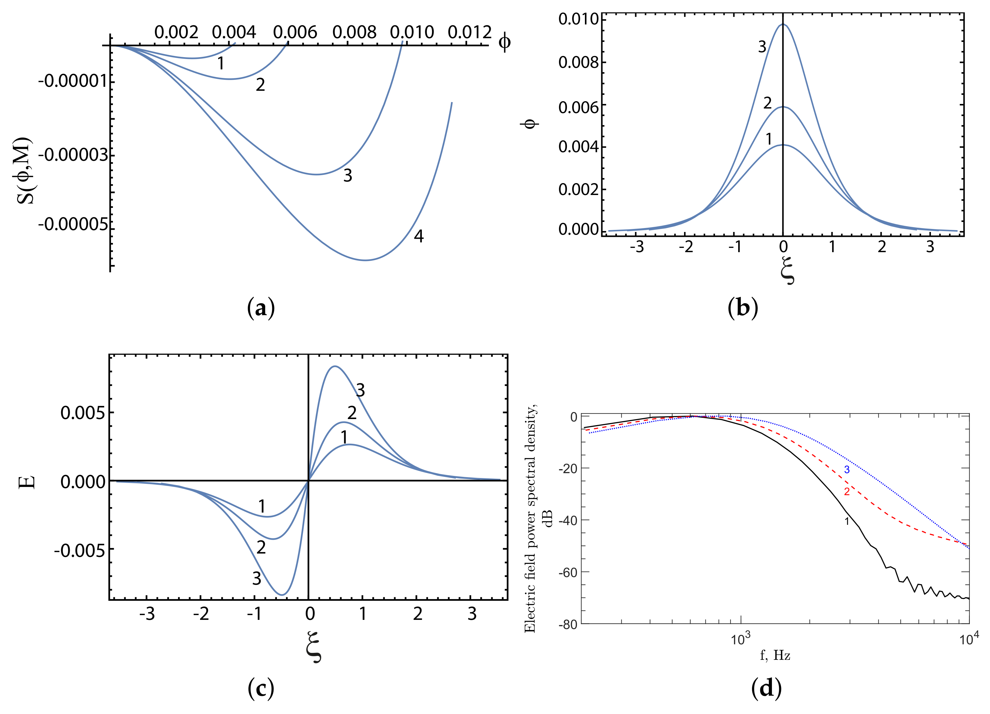
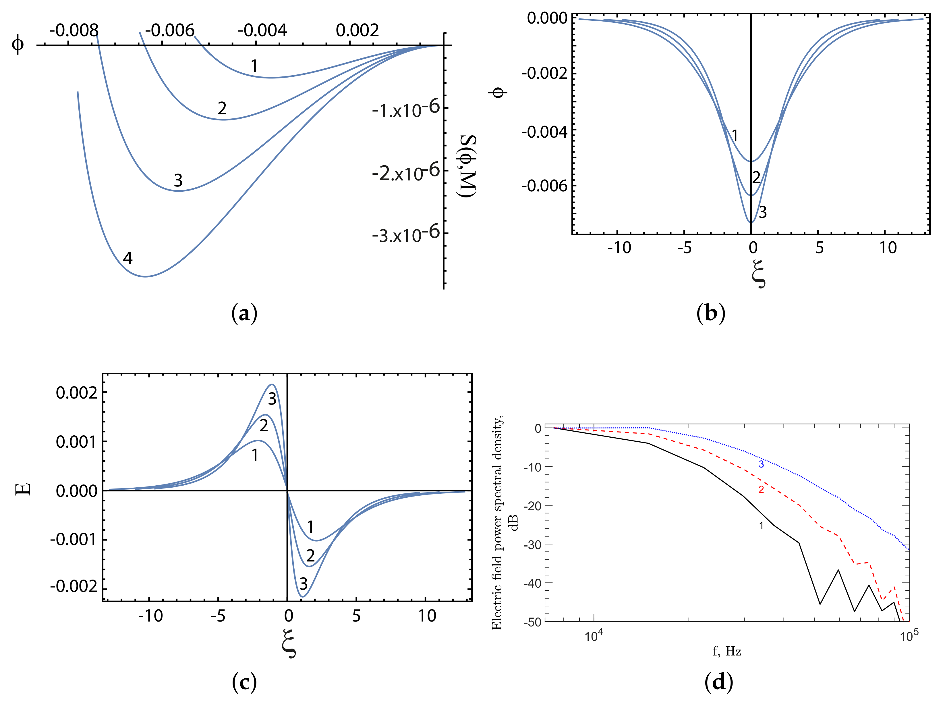
Equation (1) yields ion- and electron-acoustic soliton solutions when the Sagdeev pseudo-potential S ( ϕ , M ) satisfies the following conditions: S ( ϕ , M ) = 0, d S ( ϕ , M ) /d ϕ = 0, d 2 S ( ϕ , M ) /d ϕ 2 < 0 at ϕ = 0 ; S ( ϕ , M ) = 0 at ϕ = ϕ 0 , and S ( ϕ , M ) < 0 for 0 < ϕ < ϕ 0 ; ϕ 0 is the maximum amplitude of the soliton.
It is noted from Equation (2) that Sagdeev pseudo-potential S ( ϕ , M ) and its first derivative with respect to ϕ , i.e., d S ( ϕ , M ) /d ϕ vanish at ϕ = 0. Further, the condition d 2 S ( ϕ , M ) /d ϕ 2 < 0 at ϕ = 0 is satisfied provided M > M 0 , where M 0 is known as the critical Mach number and it satisfies the equation:
n e 1 0 μ e ( M 0 U e 1 ) 2 3 σ e 1 + n e 2 0 μ e ( M 0 U e 2 ) 2 3 σ e 2 + n c e 0 μ e M 0 2 3 σ e c + n i c 0 M 0 2 3 σ i c + n i h 0 ( M 0 U i h ) 2 3 = 0
Equation (3) yields eight roots but all the roots may not be physical. Here, we consider the real positive roots for M 0 , or the critical Mach numbers, as the negative roots have similar properties as the positive ones but propagate anti-parallel to B . In general, four critical positive Mach numbers corresponding to two (slow and fast) ion-acoustic modes and two (slow and fast) electron-acoustic modes are obtained from the numerical solution of Equation (3). However, any one or all the four modes can satisfy the soliton conditions for a given set of plasma parameters.

Numerical Results

For the numerical computation of the critical Mach numbers M 0 , and the profiles of Sagdeev pseudo-potential S ( ϕ , M ) , electric potential ϕ , and electric field E, we use the normalized parameter data set based on the observed plasma parameters, apart from the changes to the cold electron populations, during the occurrence of large-amplitude electric fields at the magnetopause by Wilder et al. [52] and used in their stability analysis. Therefore, for the input to our model, we consider the following plasma parameters: total plasma density N 0 = 20 cm 3 , cold ions density N i c = 18 cm 3 , cold ions temperature T i c = 40 eV, hot ions density N i h = 2 cm 3 , hot ions temperature T i h = 600 eV, hot ion beam speed V i h = 300 km s 1 , equal density hot electron beams with N e 1 = N e 2 = 48% (49.5%) of N 0 for cold electrons density of 4% (1%), respectively. counterstreaming hot electron beam speeds V e 1 = − V e 2 = 1325 km s 1 (corresponding to 5 eV energy), temperature of hot electron beams T e 1 = T e 2 = 80 eV, and cold electrons temperature T e c = 1 eV.
For numerical computations, the normalized plasma parameters are: n i c 0 = 0.9, n i h 0 = 0.1, σ i c = 0.07, σ i h = 1, σ e c = 0.0017, σ e 1 = σ e 2 = 0.13, U i h = 1.25, U e 1 = − U e 2 = 5.52, and n e 1 0 = n e 1 0 = 0.48 (0.495) for n e c 0 = 0.04 (0.01), respectively. The solution of Equation (3) yields four positive critical Mach numbers M 0 = 0.54225 (0.63237), 2.98223 (2.98274), 6.03499 (4.03602), 26.2828 (26.2085) for the case of n e c 0 = 0.04 (0.01), which correspond to slow ion-acoustic, fast ion-acoustic, slow electron-acoustic and fast electron-acoustic modes, respectively. The profiles of Sagdeev pseudo-potential S ( ϕ , M ) versus ϕ for M > M 0 show that fast ion-acoustic profiles are not smooth unlike for other modes, but noisy and weak (i.e., associated ϕ s are much smaller than that for slow ion-acoustic modes), and will not be considered further.
In Figure 2, we have shown the profiles of Sagdeev pseudo-potential S ( ϕ , M ) , electrostatic potential ϕ and electric field E of the slow ion-acoustic solitons computed from Equations (1) and (2) for the normalized plasma parameters for the cold electron density of n e c 0 = 0.04. Figure 2a shows the variation of Sagdeev pseudo-potential S ( ϕ , M ) for the slow ion-acoustic solitons versus the electrostatic potential ϕ for Mach number M = 0.57, 0.58, 0.60 and 0.61 for the curves 1, 2, 3 and 4, respectively. It is seen that the slow ion-acoustic solitons have positive potentials, and the maximum electrostatic potential ϕ 0 increases with the increase of the Mach number, M, as can be seen from the curves 1, 2, and 3. The soliton solution does not exist for curve 4. Hence, there is an upper value for M, say M m a x , above which slow ion-acoustic solitons cannot exist. Figure 2b shows the variation of electrostatic potential ϕ versus ξ for the slow ion-acoustic solitons. The curves 1, 2 and 3 correspond to the same Mach number M as in Figure 2a. It is seen from the curves that the amplitudes of the slow ion-acoustic solitons increase and their widths tend to decrease with the increase of M. Figure 2c shows the variation of electric field E versus ξ for the slow ion-acoustic solitons. The curves 1, 2 and 3 correspond to the same Mach number M as in Figure 2a. It is seen from the curves that the electric field E amplitudes of the slow ion-acoustic solitons increase and their widths tend to decrease with the increase of M. In Figure 2d, we have shown the fast Fourier transform (FFT) power spectra of the unnormalized electric field (in mV m 1 ) for different Mach numbers corresponding to panel c.
From Figure 2d, it is seen that EPSD (electric field power spectral density, in (mV m 1 ) 2 /Hz) expressed in dB for the slow ion-acoustic solitons has broad peaks which tend to shift towards higher frequencies with increasing the Mach number M. The peaks in spectral density occurs at f = 616 Hz, 627 Hz, and 865 Hz for M = 0.57, 0.58 and 0.60, respectively (cf. curves 1, 2 and 3). Further, it is noticed that the broad peaks in the power spectral density occur below ∼1 kHz frequencies, and then the spectral power falls sharply after the peaks. Most of the spectral power is contained in the frequency range ∼(100–1500) Hz.
Figure 3 illustrates the profiles of S ( ϕ , M ) , ϕ and E of the slow electron-acoustic solitons for the same normalized plasma parameters as in Figure 2. Figure 3a shows the variation of Sagdeev pseudo-potential S ( ϕ , M ) versus the electrostatic potential ϕ for Mach number M = 6.5, 6.7, 7.0 and 7.1 for the curves 1, 2, 3 and 4, respectively. It is seen that the slow electron-acoustic solitons have negative potentials, and the maximum electrostatic potential ϕ 0 increases with the increase in the Mach number, M, as can be seen from the curves 1, 2, and 3. The soliton solution does not exist for the M = 7.1 corresponding to curve 4. Hence, the slow electron-acoustic solitons do not exist beyond an upper value of M. Figure 3b shows the variation of electrostatic potential ϕ versus ξ for the slow electron-acoustic solitons. The curves 1, 2 and 3 correspond to the same Mach number M values as in Figure 3a. It is seen from the curves that the amplitudes of the slow electron-acoustic solitons increase and their widths tend to decrease with the increase of M. Figure 3c shows the variation of electric field E versus ξ for the slow electron-acoustic solitons. The curves 1, 2 and 3 correspond to the same Mach number M as in Figure 3a. It is seen from the curves that the electric field E amplitudes of the slow ion-acoustic solitons increase and their widths tend to decrease with the increase in M.
The power spectra of slow electron-acoustic soliton shown in Figure 3d have features similar to those of slow ion-acoustic solitons (Figure 2d, but the spectral power is less than that of slow ion-acoustic solitons (cf. E field column 6 of Table 1, and the peaks occur at higher frequencies, i.e., at f = 3659 Hz, 3772 Hz and 5911 Hz for curve 1 (M = 6.5), curve 2 (M = 6.7) and curve 3 (M = 7.0), respectively. Most of the spectral power resides in the frequency range of ∼(2–10) kHz.
In Figure 4, profiles of S ( ϕ , M ) , ϕ and E of the fast electron-acoustic solitons are shown for the same normalized plasma parameters as in Figure 2. Figure 4a shows the variation of Sagdeev pseudo-potential S ( ϕ , M ) versus the electrostatic potential ϕ for Mach number M = 26.45, 26.50, 26.55 and 26.59 for the curves 1, 2, 3 and 4, respectively. From the curves 1, 2, and 3, it is seen that the fast electron-acoustic solitons have negative potentials, and the maximum electrostatic potential ϕ 0 increases with the increase in the Mach number, M. For M = 26.59 (curve 4) and greater, the soliton solutions do not exist. Figure 4b shows the variation of electrostatic potential ϕ versus ξ for the fast electron-acoustic solitons. The curves 1, 2 and 3 corresponds to the same Mach number M values as in Figure 4a. It is seen from the curves that the amplitudes of the fast electron-acoustic solitons increase and their widths tend to decrease with the increase of M. Figure 4c shows the variation of electric field E versus ξ for the fast electron-acoustic solitons. The curves 1, 2 and 3 correspond to the same Mach number M as in Figure 4a. It is seen from the curves that for fast electron-acoustic solitons, increases in the Mach number M lead to increases in their electric field E amplitudes and decreases in their widths.
From Figure 4d, it is seen that power spectra of fast electron-acoustic soliton also have features similar to those of slow ion-acoustic solitons (Figure 2d) and slow electron-acoustic solitons (Figure 3d), but the spectral power is less than that of the slow ion-acoustic solitons (cf. E field column 6 of Table 1, and the peaks occur at still higher frequencies, i.e., at f = 7445 Hz, 7459 Hz and 14946 Hz for curve 1 (M = 26.45), curve 2 (M = 26.50) and curve 3 (M = 26.55), respectively. Here, most of the spectral power resides in the frequency range of ∼(7–30) kHz.
For the case of cold electron density of 1%, the electric field power spectral density curves of all the modes are similar but the value of the electric field power spectral density is larger by more than an order of magnitude (not shown).

2.2. Predictions of the Model

We have also computed the profiles of Sagdeev pseudo-potential S ( ϕ , M ) , electrostatic potential ϕ and electric field E of the slow ion-acoustic, slow electron-acoustic and fast electron-acoustic solitons for the case of cold electron density of n e c 0 = 0.01. The qualitative behavior of all the three soliton types is found to be similar. In Table 1 and Table 2, we list the properties of the slow ion-acoustic, slow electron-acoustic and fast electron-acoustic solitons for the cases of cold electron density of N e c = 0.04 N 0 and 0.01 N 0 , respectively. In these Tables, columns 1 and 2 describe the mode and the polarity associated with it, respectively. Column 3 gives the Mach numbers associated with the mode, Columns 4–7 give the soliton velocity, V in km s 1 , soliton width, defined as the full width at half maximum, W in m, electric field, E in mV m 1 , and electric potential, Φ in volts, respectively. Column 8 gives the range of f p e a k , the frequency where the peak power in the FFT power spectrum of the electric field occurs. Further, for the parameters of the magnetopause considered here, we get the hot ion thermal speed, C i h = 240 km s 1 , and hot ion Debye length, λ d i = 40 m.
Table 1 for the case of cold electron density N e c = 0.04 N 0 , shows that slow ion-acoustic solitons have positive potentials and the electric fields are in the range of E = (40–120) mV m 1 with solitons velocities V= (137–144) km s 1 , widths W = (59–83) m, electrostatic potentials ϕ = (2.4–5.7) V, and f p e a k (the frequency where electric field spectral power has a peak value) = (616–865) Hz. Both slow and fast electron-acoustic solitons have negative potentials with electric fields, velocity, width, electrostatic potential and frequency of spectral power peaks in the ranges of E = (10–30) mV m 1 and (12–33) mV m 1 , V = (1560–1680) km s 1 and (6348–6372) km s 1 , W = (102–158) m and (169–265) m, and ϕ = (1.3–2.5) V and (3.1–4.5) V, and f p e a k = (3659–5911) Hz and (7445–14946) Hz, respectively.
From Table 2 for the case of cold electron density N e c = 0.01 N 0 , it is seen that slow ion-acoustic solitons have positive potentials and the electric fields are in the range of E = (120–400) mV m 1 with solitons velocities V = (168–184) km s 1 , widths W = (87–123) m, and electrostatic potentials ϕ = (11–28) V. On the other hand, both slow and fast electron-acoustic solitons have negative potentials and electric fields, and spectral power frequency in the range of E = (1–3) mV m 1 and (5–30) mV m 1 , respectively, V = (1008–1044) km s 1 and (6312–6360) km s 1 , respectively, W = (114–177) m and (165–400) m, respectively, and ϕ = (0.15–0.27) V and (1.5–4.2) V, respectively, and f p e a k = (1513–2351) Hz and (4738–9548) Hz, respectively. Further, from Table 1 and Table 2, it is clear that for slow ion-acoustic solitons, their velocities V, electric fields E and electrostatic potential ϕ are increased, but their widths W remain unaffected and f p e a k are decreased when the cold electron density N e c is changed from 0.04 N 0 to 0.01 N 0 . On the other hand, W, V, E, ϕ and f p e a k associated with both slow and fast electron-acoustic solitons are generally increased for N e c = 0.04 N 0 as compared to the case of N e c = 0.01 N 0 .

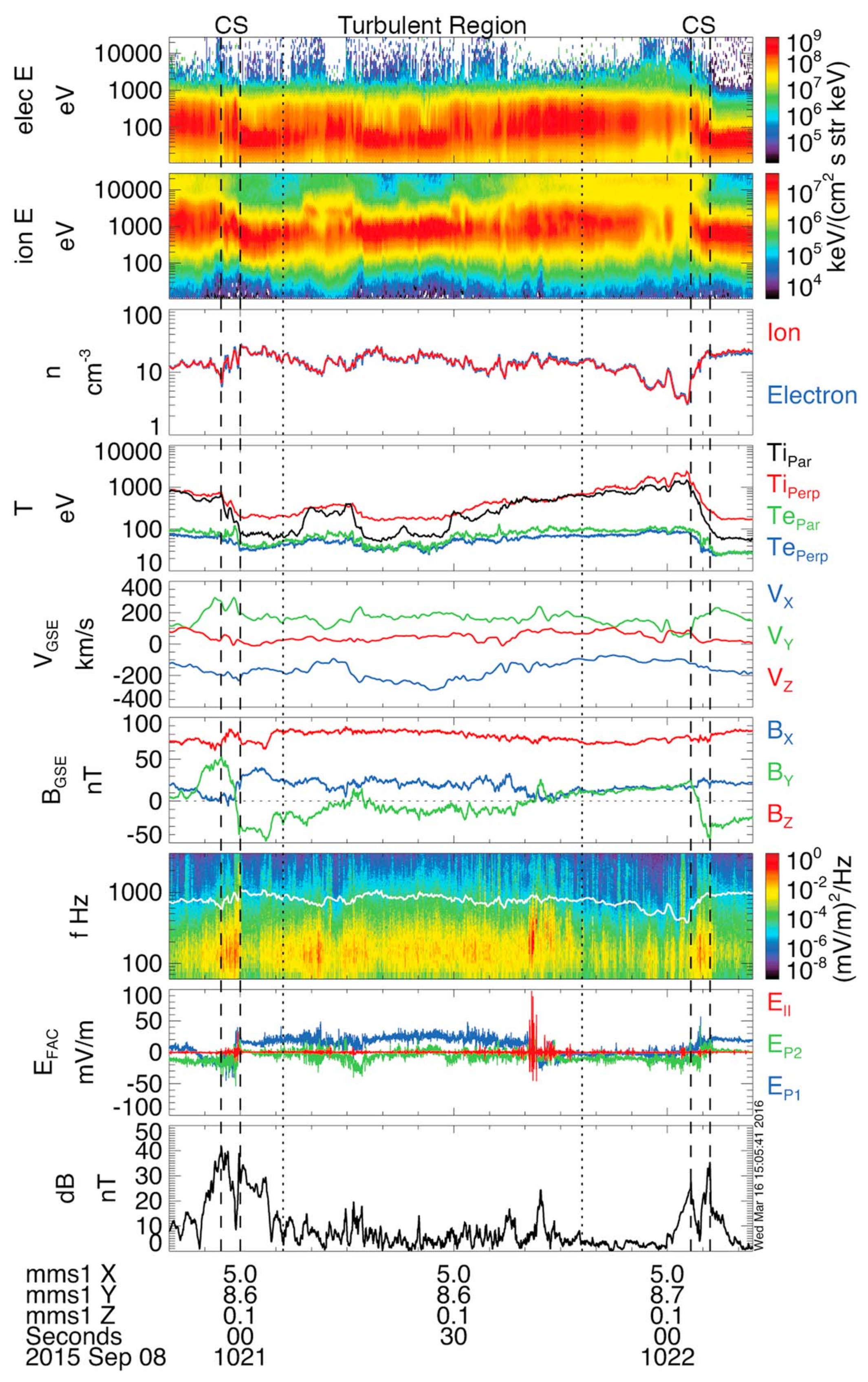
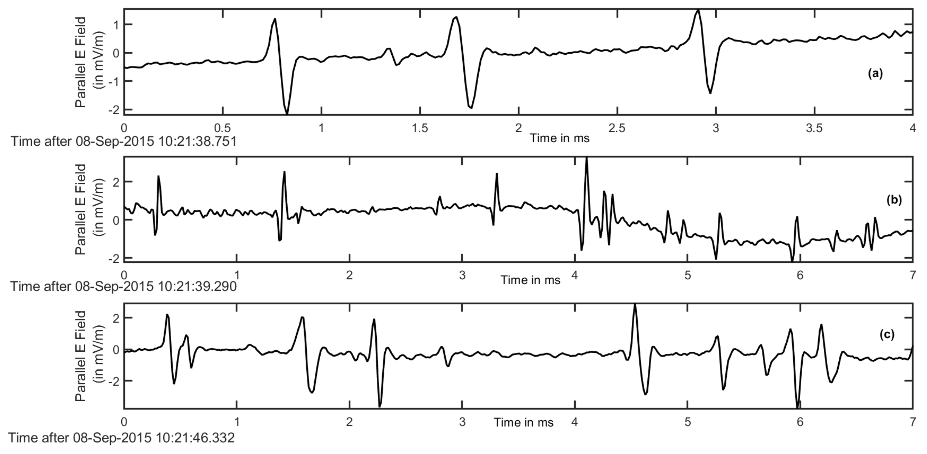
2.3. Comparison of Theoretical Predictions with Observations of Large Amplitude Electrostatic Waves at the Magnetopause

Wilder et al. [52] reported the observation of large-amplitude electrostatic waves propagating parallel to the background magnetic field at the magnetopause in the region where there is an intermixing of magnetosheath and magnetospheric plasmas on 8 September 2015 during (10:20:50–10:22:10) UT by the MMS spacecraft. During the interval 10:21:40 UT to 10:21:42 UT, the electric field power spectral density was concentrated between frequencies range of ∼(100–1000) Hz with peak electric field amplitude in the range of ∼(25–100) mV m 1 . Further, high-frequency waves with f > 1 kHz are also observed but with much lower intensity (cf. Figures 1 and 2 of Wilder et al. [52]).
These observations are explainable in terms of slow ion-acoustic solitons. From Figure 2c,d and Table 1 (which are for case of 4% cold electrons density), it is seen that soliton electric fields E are in the range of (40–120) mV m 1 and the maximum electric field power spectral density occurs in the frequency range ∼(100–1500) Hz. This is an excellent agreement between the observations and theory. However, the predicted E field for M = 0.60 is 120 mV m 1 , which is higher than that observed [52]. The agreement between theory and observations deteriorates for the case of 1% cold electron density as seen from Table 2.
Slow and fast electron-acoustic solitons may be relevant in explaining the low-intensity, high-frequency f > 1 kHz waves observed by Wilder et al. [52]. Their electric field’s FFT power spectra has maximum power (which is much less than the slow ion-acoustic solitons) in the frequency range ∼(3659–5911) Hz (for slow electron-acoustic) and ∼(7445–14946) Hz (fast electron-acoustic) (cf. Table 1, Figure 3 and Figure 4) for the case of 4% cold electron density. For the case of 1% cold electron density (cf. Table 2), the electric fields Es are smaller for both slow and fast electron-acoustic solitons than the case of 4% cold electrons density, and the FFT power spectra has maximum power in frequency range ∼(1513–2351) Hz (for slow electron-acoustic) and ∼(4738–9548) Hz (fast electron-acoustic). We note that the maximum frequency of the FFT in Figure 1 (and Figure 2 of Wilder et al. [52]) is ∼3 kHz (though in principle up to 4 kHz should be resolved from the data), and in Wilder et al. [52] Figure 2, the power seems to fall off above this. It is fair to say that the slow and fast electron-acoustic solitons allow for the existence of low-intensity, high-frequency waves 1.5 kHz and 3.6 kHz for the case of cold electrons having density of 1% and 4%, respectively. However, more support from the data is needed.
We would like to point out that from wave spectra alone it is not clear whether the observed waves are simply ion-acoustic waves as suggested by Wilder et al. [52], or whether they actually have formed into solitary structures. We searched the MMS burst waveform highest resolution HMFE data sampled at 65 kHz to check whether the waves had evolved into solitary structures. Unfortunately, there are no high-resolution waveform HMFE data for the wave interval of our study, i.e., on 8 September 2015 during the interval 10:21:40 UT to 10:21:42 UT. However, highest-resolution HMFE electric field Level 2 data are available both before and after this interval, which we have plotted in Figure 5. Panels a and b are before, and Panel c is after the observed wave interval of interest. It is clear from Panels a, b and c of Figure 5 that the observed waves have evolved into solitary structures. We expect the same behavior for the interval between Panel b and Panel c. This lends support to the soliton model proposed here, but an alternative explanation in terms of ion and electron phase space holes is also a possibility.

3. Conclusions

We have described a fluid model, based on Sagdeev pseudo-potential technique, to investigate the properties of nonlinear ion- and electron-acoustic solitons in a plasma system consisting of five components, namely, cold ions, hot ion beam, two hot electron beams counter streaming along the ambient magnetic field, and the cold electrons. This plasma system represents quite well the magnetopause turbulent region, where the magnetosheath and magnetospheric plasmas are intermixed. We use this model to explain the large amplitude electrostatic waves observed by Wilder et al. [52] at the magnetopause by the MMS spacecraft on 8 September 2015. When we take the observed plasma parameters for the times between 10:21:40 UT and 10:21:42 UT on 8 September 2015 as input for our theoretical model, it predicts three types of stable solitons, namely, slow ion-acoustic, slow and fast electron-acoustic solitons. The fourth type of fast ion-acoustic solitons do not exist for the parameters considered here.
The properties of the electrostatic waves propagating parallel to the magnetic field observed by MMS on 8 September 2015 during the times between 10:21:40 UT and 10:21:42 UT, as discussed by Wilder et al. [52], are: large amplitude electrostatic waves in the frequency range f (100–1000) Hz having electric fields E (25–100) mV m 1 . There are much weaker high-frequency ( f > 1 kHz) waves having electric field power spectral density which is smaller than that of low-frequency waves by four to six orders of magnitude. From Table 1 and Figure 2d, one can see that for 4% cold electron density case, slow ion-acoustic solitons have electric field E = (40–120) mV m 1 and most of the electric field power density is contained in the frequency range 100 Hz < f < 1500 Hz. This shows a good agreement with the observations.
The low-intensity high-frequency ( f > 1 kHz waves could be due to slow and fast electron-acoustic solitons as their electric fields are much smaller than those of slow ion-acoustic modes (cf. Table 1 and Table 2). For the case of 4% cold electron density, the FFT power spectra of their electric fields shows that most of the power is concentrated in the frequency range of 3.6 kHz < f < 5.9 kHz and 7.4 kHz < f < 15 kHz for the slow and fast electron-acoustic solitons, respectively (cf. Figure 3d and Figure 4d). For the case of 1% cold electron density, the FFT power spectra has maximum power in frequency range 1.5 kHz < f < 24 kHz and 4.7 kHz < f < 9.5 kHz for the slow and fast electron-acoustic solitons, respectively (cf. Table 2).
To summarize, it is proposed that the slow ion-acoustic solitons studied here can explain the observations of large amplitude electrostatic waves in the frequency range of f = (100–1000) Hz with electric field of up to E 100 mV m 1 propagating parallel to the ambient magnetic field at the magnetopause reported by Wilder et al. [52]. The low-intensity, high-frequency waves with f > 1 kHz, which were also observed at the time of large amplitude low-frequency waves could be explained in terms of slow and fast electron-acoustic solitons. We would like to emphasize that though the soliton model proposed here can explain the observations of large amplitude electrostatic waves observed by Wilder et al., (2016), in no way it implies that an alternative theory in terms of ion and electron phase space hole cannot do the same. However, there is no theory based on ion/electron phase space holes pertaining to the observations of Wilder et al., (2016) available at present.

Author Contributions

Conceptualization, G.S.L.; methodology, G.S.L. and S.S.; writing—original draft preparation, G.S.L., S.S., T.S. and S.D.; software and formal analysis, R.R., S.S., T.S. and S.D.; validation, G.S.L., S.S., T.S. and S.D.; writing—review and editing, G.S.L., S.S., T.S. and S.D. All authors have read and agreed to the published version of the manuscript.

Funding

Indian National Science Academy: INSA/SP/HS/2021, DST/INSPIRE/04/2021/000366.

Institutional Review Board Statement

Not applicable.

Informed Consent Statement

Not applicable.

Data Availability Statement

Data used in this paper are in the public domain and can be found in the paper by Wilder et al., (2016), Observations of large-amplitude, parallel, electrostatic waves associated with the Kelvin-Helmholtz instability by the magnetospheric multiscale mission, Geophys. Res. Lett., 43, 8859–8866, https://doi.org/10.1002/2016GL070404. The highest resolution HMFE Electric Field, Level 2 burst mode data from MMS1 used in Figure 5 can be downloaded from the website: https://lasp.colorado.edu/mms/sdc/public/ (accessed on 28 February 2023).

Acknowledgments

GSL thanks the Indian National Science Academy, New Delhi for support under the INSA—Honorary Scientist Scheme. RR thanks Department of Science and Technology (DST), Government of India, India for the support under INSPIRE Faculty Fellowship. The authors would like to thank Bharati Kakad for her help in FFT. We acknowledge the use of highest-resolution HMFE Electric Field, Level 2 burst mode data from MMS mission. Data can be accessed from the website: https://lasp.colorado.edu/mms/sdc/public/ (accessed on 28 February 2023).

Conflicts of Interest

The authors declare no conflict of interest.

References

  1. Gurnett, D.A.; Anderson, R.R.; Tsurutani, B.T.; Smith, E.J.; Paschmann, G.; Haerendel, G.; Bame, S.J.; Russell, C.T. Plasma wave turbulence at the magnetopause: Observations from ISEE 1 and 2. J. Geophys. Res. 1979, 84, 7043–7058. [Google Scholar] [CrossRef]
  2. Matsumoto, H.; Deng, X.H.; Kojima, H.; Anderson, R.R. Observation of Electrostatic Solitary Waves associated with reconnection on the dayside magnetopause boundary. Geophys. Res. Lett. 2003, 30, 1326. [Google Scholar] [CrossRef]
  3. Graham, D.B.; Khotyaintsev, Y.V.; Vaivads, A.; André, M. Electrostatic solitary waves with distinct speeds associated with asymmetric reconnection. Geophys. Res. Lett. 2015, 42, 215–224. [Google Scholar] [CrossRef]
  4. Matsumoto, H.; Kojima, H.; Miyatake, T.; Omura, Y.; Okada, M.; Nagano, I.; Tsutsui, M. Electrostatic solitary waves (ESW) in the magnetotail: BEN wave forms observed by GEOTAIL. Geophys. Res. Lett. 1994, 21, 2915–2918. [Google Scholar] [CrossRef]
  5. Kojima, H.; Matsumoto, H.; Chikuba, S.; Horiyama, S.; Ashour-Abdalla, M.; Anderson, R.R. Geotail waveform observations of broadband/narrowband electrostatic noise in the distant tail. J. Geophys. Res. 1997, 102, 14439–14455. [Google Scholar] [CrossRef]
  6. Pickett, J.S.; Menietti, J.D.; Gurnett, D.A.; Tsurutani, B.; Kintner, P.M.; Klatt, E.; Balogh, A. Solitary potential structures observed in the magnetosheath by the Cluster spacecraft. Nonlin. Process. Geophys. 2003, 10, 3–11. [Google Scholar] [CrossRef]
  7. Pickett, J.S.; Chen, L.J.; Kahler, S.W.; Santolík, O.; Gurnett, D.A.; Tsurutani, B.T.; Balogh, A. Isolated electrostatic structures observed throughout the Cluster orbit: Relationship to magnetic field strength. Ann. Geophys. 2004, 22, 2515–2523. [Google Scholar] [CrossRef]
  8. Pickett, J.S.; Chen, L.J.; Kahler, S.W.; Santolík, O.; Goldstein, M.L.; Lavraud, B.; Décréau, P.M.E.; Kessel, R.; Lucek, E.; Lakhina, G.S.; et al. On the generation of solitary waves observed by Cluster in the near-Earth magnetosheath. Nonlinear Process. Geophys. 2005, 12, 181–193. [Google Scholar] [CrossRef]
  9. Holmes, J.C.; Ergun, R.E.; Newman, D.L.; Wilder, F.D.; Sturner, A.P.; Goodrich, K.A.; Torbert, R.B.; Giles, B.L.; Strangeway, R.J.; Burch, J.L. Negative potential solitary structures in the magnetosheath with large parallel width. J. Geophys. Res. 2018, 123, 132–145. [Google Scholar] [CrossRef]
  10. Lakhina, G.S.; Tsurutani, B.T.; Kojima, H.; Matsumoto, H. “Broadband” plasma waves in the boundary layers. J. Geophys. Res. 2000, 105, 27791–27831. [Google Scholar] [CrossRef]
  11. Bernstein, I.B.; Greene, J.M.; Kruskal, M.D. Exact Nonlinear Plasma Oscillations. Phys. Rev. 1957, 108, 546–550. [Google Scholar] [CrossRef]
  12. Schamel, H. Stationary solitary, snoidal and sinusoidal ion acoustic waves. Plasma Phys. 1972, 14, 905–924. [Google Scholar] [CrossRef]
  13. Omura, Y.; Matsumoto, H.; Miyake, T.; Kojima, H. Electron beam instabilities as generation mechanism of electrostatic solitary waves in the magnetotail. J. Geophys. Res. 1996, 101, 2685–2697. [Google Scholar] [CrossRef]
  14. Schamel, H. Particle trapping: A key requisite of structure formation and stability of Vlasov–Poisson plasmas. Phys. Plasmas 2015, 22, 042301. [Google Scholar] [CrossRef]
  15. Hutchinson, I.H. Electron holes in phase space: What they are and why they matter. Phys. Plasmas 2017, 24, 055601. [Google Scholar] [CrossRef]
  16. Goldman, M.V.; Oppenheim, M.M.; Newman, D.L. Nonlinear two-stream instabilities as an explanation for auroral bipolar wave structures. Geophys. Res. Lett. 1999, 26, 1821–1824. [Google Scholar] [CrossRef]
  17. Oppenheim, M.; Newman, D.L.; Goldman, M.V. Evolution of Electron Phase-Space Holes in a 2D Magnetized Plasma. Phys. Rev. Lett. 1999, 83, 2344–2347. [Google Scholar] [CrossRef]
  18. Muschietti, L.; Ergun, R.E.; Roth, I.; Carlson, C.W. Phase-space electron holes along magnetic field lines. Geophys. Res. Lett. 1999, 26, 1093–1096. [Google Scholar] [CrossRef]
  19. Singh, N. Space-time evolution of electron-beam driven electron holes and their effects on the plasma. Nonlinear Process. Geophys. 2003, 10, 53–63. [Google Scholar] [CrossRef]
  20. Ergun, R.E.; Carlson, C.W.; McFadden, J.P.; Mozer, F.S.; Muschietti, L.; Roth, I.; Strangeway, R.J. Debye-Scale Plasma Structures Associated with Magnetic-Field-Aligned Electric Fields. Phys. Rev. Lett. 1998, 81, 826–829. [Google Scholar] [CrossRef]
  21. Franz, J.R.; Kintner, P.M.; Pickett, J.S.; Chen, L.J. Properties of small-amplitude electron phase-space holes observed by Polar. J. Geophys. Res. 2005, 110, A09212. [Google Scholar] [CrossRef]
  22. Chen, L.J.; Pickett, J.; Kintner, P.; Franz, J.; Gurnett, D. On the width-amplitude inequality of electron phase space holes. J. Geophys. Res. 2005, 110, A09211. [Google Scholar] [CrossRef]
  23. Omura, Y.; Kojima, H.; Matsumoto, H. Computer simulation of electrostatic solitary waves: A nonlinear model of broadband electrostatic noise. Geophys. Res. Lett. 1994, 21, 2923–2926. [Google Scholar] [CrossRef]
  24. Singh, N.; Schunk, R.W. Plasma response to the injection of an electron beam. Plasma Phys. Control Fusion 1984, 26, 859. [Google Scholar] [CrossRef]
  25. Singh, N.; Thiemann, H.; Schunk, R.W. Simulations of auroral plasma processes: Electric fields, waves and particles. Planet. Space Sci. 1987, 35, 353–395. [Google Scholar] [CrossRef]
  26. Singh, N.; Loo, S.M.; Wells, E. Electron hole structure and its stability depending on plasma magnetization. J. Geophys. Res. 2001, 106, 21183–21198. [Google Scholar] [CrossRef]
  27. Ergun, R.E.; Carlson, C.W.; McFadden, J.P.; Mozer, F.S.; Delory, G.T.; Peria, W.; Chaston, C.C.; Temerin, M.; Roth, I.; Muschietti, L.; et al. FAST satellite observations of large-amplitude solitary structures. Geophys. Res. Lett. 1998, 25, 2041–2044. [Google Scholar] [CrossRef]
  28. Muschietti, L.; Roth, I.; Carlson, C.W.; Ergun, R.E. Transverse Instability of Magnetized Electron Holes. Phys. Rev. Lett. 2000, 85, 94–97. [Google Scholar] [CrossRef]
  29. Graham, D.B.; Khotyaintsev, Y.V.; Vaivads, A.; André, M. Electrostatic solitary waves and electrostatic waves at the magnetopause. J. Geophys. Res. Space Phys. 2016, 121, 3069–3092. [Google Scholar] [CrossRef]
  30. Mozer, F.S.; Agapitov, O.V.; Giles, B.; Vasko, I. Direct Observation of Electron Distributions inside Millisecond Duration Electron Holes. Phys. Rev. Lett. 2018, 121, 135102. [Google Scholar] [CrossRef]
  31. Steinvall, K.; Khotyaintsev, Y.V.; Graham, D.B.; Vaivads, A.; Lindqvist, P.A.; Russell, C.T.; Burch, J.L. Multispacecraft analysis of electron holes. Geophys. Res. Lett. 2019, 46, 55–63. [Google Scholar] [CrossRef]
  32. Lotekar, A.; Vasko, I.Y.; Mozer, F.S.; Hutchinson, I.; Artemyev, A.V.; Bale, S.D.; Bonnell, J.W.; Ergun, R.; Giles, B.; Khotyaintsev, Y.V.; et al. Multisatellite MMS analysis of electron holes in the Earth’s magnetotail: Origin, properties, velocity gap, and transverse instability. J. Geophys. Res. Space Phys. 2020, 125, e2020JA028066. [Google Scholar] [CrossRef]
  33. Wang, R.; Vasko, I.Y.; Artemyev, A.V.; Holley, L.C.; Kamaletdinov, S.R.; Lotekar, A.; Mozer, F.S. Multisatellite observations of ion holes in the Earth’s plasma sheet. Geophys. Res. Lett. 2022, 49, e2022GL097919. [Google Scholar] [CrossRef]
  34. Sagdeev, R.Z. Cooperative Phenomena and Shock Waves in Collisionless Plasmas. In Reviews of Plasma Physics; Leontovich, M.A., Ed.; Consultants Bureau: New York, NY, USA, 1966; Volume 4, pp. 23–91. [Google Scholar]
  35. Ghosh, S.S.; Iyengar, A.N.S. Anomalous width variations for ion acoustic rarefactive solitary waves in a warm ion plasma with two electron temperatures. Phys. Plasmas 1997, 4, 3204–3210. [Google Scholar] [CrossRef]
  36. Ghosh, S.S.; Lakhina, G.S. Anomalous width variation of rarefactive ion acoustic solitary waves in the context of auroral plasmas. Nonlinear Process. Geophys. 2004, 11, 219–228. [Google Scholar] [CrossRef]
  37. Singh, S.V.; Reddy, R.V.; Lakhina, G.S. Broadband electrostatic noise due to nonlinear electron-acoustic waves. Adv. Space Res. 2001, 28, 1643–1648. [Google Scholar] [CrossRef]
  38. Ghosh, S.S.; Pickett, J.S.; Lakhina, G.S.; Winningham, J.D.; Lavraud, B.; Décréau, P.M.E. Parametric analysis of positive amplitude electron acoustic solitary waves in a magnetized plasma and its application to boundary layers. J. Geophys. Res. 2008, 113, A06218. [Google Scholar] [CrossRef]
  39. Lakhina, G.S.; Kakad, A.P.; Singh, S.V.; Verheest, F. Ion- and electron-acoustic solitons in two-electron temperature space plasmas. Phys. Plasmas 2008, 15, 062903. [Google Scholar] [CrossRef]
  40. Lakhina, G.S.; Singh, S.V.; Kakad, A.P.; Verheest, F.; Bharuthram, R. Study of nonlinear ion- and electron-acoustic waves in multi-component space plasmas. Nonlinear Process. Geophys. 2008, 15, 903–913. [Google Scholar] [CrossRef]
  41. Devanandhan, S.; Singh, S.V.; Lakhina, G.S. Electron acoustic solitary waves with kappa-distributed electrons. Phys. Scr. 2011, 84, 025507. [Google Scholar] [CrossRef]
  42. Maharaj, S.K.; Bharuthram, R.; Singh, S.V.; Lakhina, G.S. Existence domains of arbitrary amplitude nonlinear structures in two-electron temperature space plasmas. I. Low-frequency ion-acoustic solitons. Phys. Plasmas 2012, 19, 072320. [Google Scholar] [CrossRef]
  43. Dillard, C.S.; Vasko, I.Y.; Mozer, F.S.; Agapitov, O.V.; Bonnell, J.W. Electron-acoustic solitary waves in the Earth’s inner magnetosphere. Phys. Plasmas 2018, 25, 022905. [Google Scholar] [CrossRef]
  44. Lakhina, G.S.; Singh, S.V.; Rubia, R. A mechanism for electrostatic solitary waves observed in the reconnection jet region of the Earth’s magnetotail. Adv. Space Res. 2021, 68, 1864–1875. [Google Scholar] [CrossRef]
  45. Lakhina, G.S.; Singh, S.V.; Rubia, R.; Sreeraj, T. A review of nonlinear fluid models for ion-and electron-acoustic solitons and double layers: Application to weak double layers and electrostatic solitary waves in the solar wind and the lunar wake. Phys. Plasmas 2018, 25, 080501. [Google Scholar] [CrossRef]
  46. Lakhina, G.S.; Singh, S.V.; Rubia, R.; Devanandhan, S. Electrostatic Solitary Structures in Space Plasmas: Soliton Perspective. Plasma 2021, 4, 681–731. [Google Scholar] [CrossRef]
  47. Ergun, R.E.; Holmes, J.C.; Goodrich, K.A.; Wilder, F.D.; Stawarz, J.E.; Eriksson, S.; Newman, D.L.; Schwartz, S.J.; Goldman, M.V.; Sturner, A.P.; et al. Magnetospheric Multiscale observations of large-amplitude, parallel, electrostatic waves associated with magnetic reconnection at the magnetopause. Geophys. Res. Lett. 2016, 43, 5626–5634. [Google Scholar] [CrossRef]
  48. Ergun, R.E.; Goodrich, K.A.; Wilder, F.D.; Holmes, J.C.; Stawarz, J.E.; Eriksson, S.; Sturner, A.P.; Malaspina, D.M.; Usanova, M.E.; Torbert, R.B.; et al. Magnetospheric multiscale satellites observations of parallel electric fields associated with magnetic reconnection. Phys. Rev. Lett. 2016, 116, 235102. [Google Scholar] [CrossRef]
  49. Rufai, O.R.; Khazanov, G.V.; Singh, S.V.; Lakhina, G.S. Large-amplitude electrostatic fluctuations at the Earth’s magnetopause with a vortex-like distribution of hot electrons. Results Phys. 2022, 35, 105343. [Google Scholar] [CrossRef]
  50. Rufai, O.R.; Khazanov, G.V.; Singh, S.V. Finite amplitude electron-acoustic waves in the electron diffusion region. Results Phys. 2021, 24, 104041. [Google Scholar] [CrossRef]
  51. Rufai, O.R.; Singh, S.V.; Lakhina, G.S. Nonlinear electrostatic structures and stopbands in a three-component magnetosheath plasma. Astrophys. Space Sci. 2023, 368, 35. [Google Scholar] [CrossRef]
  52. Wilder, F.D.; Ergun, R.E.; Schwartz, S.J.; Newman, D.L.; Eriksson, S.; Stawarz, J.E.; Goldman, M.V.; Goodrich, K.A.; Gershman, D.J.; Malaspina, D.M.; et al. Observations of large-amplitude, parallel, electrostatic waves associated with the Kelvin-Helmholtz instability by the magnetospheric multiscale mission. Geophys. Res. Lett. 2016, 43, 8859–8866. [Google Scholar] [CrossRef]
  53. Nakamura, T.K.M.; Daughton, W.; Karimabadi, H.; Eriksson, S. Three-dimensional dynamics of vortex-induced reconnection and comparison with THEMIS observations. J. Geophys. Res. Space Phys. 2013, 118, 5742–5757. [Google Scholar] [CrossRef]
  54. Kindel, J.M.; Kennel, C.F. Topside current instabilities. J. Geophys. Res. 1971, 76, 3055. [Google Scholar] [CrossRef]
  55. Lakhina, G.S.; Singh, S.V.; Kakad, A.P.; Pickett, J.S. Generation of electrostatic solitary waves in the plasma sheet boundary layer. J. Geophys. Res. 2011, 116, A10218. [Google Scholar] [CrossRef]
  56. Lakhina, G.S.; Singh, S.V.; Kakad, A.P. Ion acoustic solitons/double layers in two-ion plasma revisited. Phys. Plasmas 2014, 21, 062311. [Google Scholar] [CrossRef]
  57. Lakhina, G.S.; Singh, S.V.; Rubia, R. A new class of Ion-acoustic solitons that can exist below critical Mach number. Phys. Scr. 2020, 95, 105601. [Google Scholar] [CrossRef]
Figure 1. Overview example of ESWs observed during a single period of K–H instability oscillations on 8 September 2015 by MMS spacecraft. From top to bottom, electron and ion omnidirectional energy spectra, electron and ion number density, electron and ion temperature, ion bulk velocity in geocentric solar ecliptic (GSE) coordinates, magnetic field vector in GSE, electric field power spectral density (EPSD) in (mV/m) 2 /Hz, the electric field in field-aligned coordinates(FAC), and total magnetic field fluctuations. The white line on the spectrum is the ion plasma frequency, the dashed vertical black lines indicate crossings of the vortex-induced current sheets, and the dotted vertical lines indicate the interval with turbulent region where the magnetopause and magnetosheath plasmas are intermixed. (Figure reprinted with permission from [52]).
Plasma 06 00024 g001
Figure 2. Panel (a) shows variation of Sagdeev pseudo-potential S ( ϕ , M ) for the slow ion-acoustic solitons versus the electrostatic potential ϕ , for the cold electron density of n e c 0 = 0.04 and for n i c 0 = 0.9, n i h 0 = 0.1, σ i c = 0.07, σ i h = 1, σ e c = 0.0017, σ e 1 = σ e 2 = 0.13, U i h = 1.25, U e 1 = U e 2 = 5.52, and n e 1 0 = n e 1 0 = 0.48, and for Mach number M = 0.57, 0.58, 0.60 and 0.61 for the curves 1, 2, 3 and 4, respectively. Curve 4 shows that slow ion-acoustic solitons do not exist for M 0.61. Panel (b) shows soliton profiles of electrostatic potential ϕ versus ξ for the Mach numbers corresponding to curves 1, 2 and 3 of Panel (a). Panel (c) shows profiles of the electric field E versus ξ for the Mach numbers corresponding to curves 1, 2 and 3 of Panel (a). Panel (d) shows FFT power spectra of the unnormalized slow ion-acoustic solitons electric field E (in mV m 1 ). The x-axis represents the frequency, f, in Hz. The y-axis represents the electric field power spectral density ((mV m 1 ) 2 /Hz), normalized with the peak power spectral density, expressed in units of decibel, dB. The power spectral density peaks at f = 616 Hz, 627 Hz, and 865 Hz for M = 0.57 (curve 1), 0.58 (curve 2) and 0.60 (curve 3), respectively.
Plasma 06 00024 g002
Figure 3. Panel (a) shows variation of Sagdeev pseudo-potential S ( ϕ , M ) for the slow electron-acoustic solitons versus the electrostatic potential ϕ , for the same plasma parameters as in Figure 2 and for Mach number M = 6.5, 6.7, 7.0 and 7.1 for the curves 1, 2, 3 and 4, respectively. Curve 4 shows that slow electron-acoustic solitons do not exist for M 7.1. Panel (b) shows soliton profiles of electrostatic potential ϕ versus ξ for the Mach numbers corresponding to curves 1, 2 and 3 of Panel (a). Panel (c) shows profiles of the electric field E versus ξ for the Mach numbers corresponding to curves 1, 2 and 3 of Panel (a). Panel (d) shows FFT power spectra of the unnormalized slow electron-acoustic solitons electric field E (in mV m 1 ) for the Mach numbers corresponding to panel c of Figure 3, and in the same format as that of Figure 2d.
Plasma 06 00024 g003
Figure 4. Panel (a) shows variation of Sagdeev pseudo-potential S ( ϕ , M ) for the fast electron-acoustic solitons versus the electrostatic potential ϕ , for the same plasma parameters as in Figure 2 and for Mach number M = 26.45, 26.50, 26.55 and 26.59 for the curves 1, 2, 3 and 4, respectively. Curve 4 shows that fast electron-acoustic solitons do not exist for M 26.59. Panels (b,c) show profiles of electrostatic potential ϕ and electric field E versus ξ , respectively, for the Mach numbers corresponding to curves 1, 2 and 3 of Panel (a). Panel (d) shows FFT power spectra of the unnormalized fast electron-acoustic solitons electric field E (in mV m 1 ) in the same format as that of Figure 2d.
Plasma 06 00024 g004
Figure 5. Plot of parallel electric field from MMS1 highest resolution HMFE Electric Field, Level 2 burst mode data sampled at 65 kHz. The y-axis shows the parallel electric field in mV/m and the x-axis represents the time in milliseconds after the start of the event.
Plasma 06 00024 g005
Table 1. Properties of the slow ion-acoustic, slow electron-acoustic and fast electron-acoustic solitons for the case of cold electron density of N e c = 0.04 N 0 for the magnetopause parameters observed by MMS spacecraft by Wilder et al. [52]: N 0 = 20 cm 3 , cold ions density N i c = 18 cm 3 , cold ions temperature T i c = 40 eV, hot ions density N i c = 2 cm 3 , hot ions temperature T i h = 600 eV, hot ion beam speed V i h = 300 km s 1 , N e 1 = N e 2 = 0.48 N 0 , cold electron density N e c = 0.04 N 0 , V e 1 = V e 2 = 1325 km s 1 , T e 1 = T e 2 = 80 eV, and T e c = 1 eV. Then, we get the hot ion thermal speed, C i h = 240 km s 1 , and hot ion Debye length, λ d i = 40 m.
ModesPolarityMach
Number
V
(km s 1 )
W
(m)
E
(mV m 1 )
Φ
(V)
f peak
(Hz)
Slow ion-acousticPositive0.5713783402.4616
0.5813972603.6627
0.60144591205.7865
Slow electron-acousticNegative6.51560158101.33659
6.71608134151.83772
7.01680102302.55911
Fast electron-acousticNegative26.456348265123.17445
26.506360211213.87459
26.556372169334.514,946
Table 2. Properties of the slow ion-acoustic, slow electron-acoustic and fast electron-acoustic solitons for the case of cold electron density of N e c = 0.01 N 0 , N e 1 = N e 2 = 0.495 N 0 and for all other plasma parameters as given in Table 1.
ModesPolarityMach
Number
V
(km s 1 )
W
(m)
E
(mV m 1 )
Φ
(V)
f peak
(Hz)
Slow ion-acousticPositive0.7016812312011504
0.751809732024541
0.7651848740028551
Slow electron-acousticNegative4.20100817710.151513
4.30103213120.232324
4.35104411430.272351
Fast electron-acousticNegative26.30631240051.54738
26.406336240153.07134
26.506360165304.29548
Disclaimer/Publisher’s Note: The statements, opinions and data contained in all publications are solely those of the individual author(s) and contributor(s) and not of MDPI and/or the editor(s). MDPI and/or the editor(s) disclaim responsibility for any injury to people or property resulting from any ideas, methods, instructions or products referred to in the content.

