
Fundamentals and Applications of Nonthermal Plasma Fluid Flows: A Review
Department of Mechanical Engineering, Osaka Metropolitan University, 1-1 Gakuen-cho, Sakai 599-8531, Japan
Plasma 2023, 6(2), 277-307; https://doi.org/10.3390/plasma6020020
Submission received: 24 January 2023
/
Revised: 23 April 2023
/
Accepted: 4 May 2023
/
Published: 10 May 2023
(This article belongs to the Special Issue Feature Papers in Plasma Sciences)
Abstract
:A review is presented to integrate fluid engineering, heat transfer engineering, and plasma engineering treated in the fields of mechanical engineering, chemical engineering, and electrical engineering. A basic equation system for plasma heat transfer fluids is introduced, and its characteristics are explained. In such reviews, generally, the gap between fundamentals and application is large. Therefore, the author attempts to explain the contents from the standpoint of application. The derivation of formulas and basic equations are presented with examples of application to plasmas. Furthermore, the heat transfer mechanisms of equilibrium and nonequilibrium plasmas are explained with reference to the basic equation system and concrete examples of analyses.
1. Introduction
Nonthermal plasma flows have been widely applied in various industries. However, the gap between fundamentals and applications is large. To design and predict the performance of industrial plasma equipment, numerical simulation or prediction for nonthermal plasma fluid flows is important and necessary. This study aims to integrate fluid engineering, heat transfer engineering, and plasma engineering treated in the fields of mechanical engineering, chemical engineering, and electrical engineering. A basic equation system for plasma heat transfer fluids is introduced, and its characteristics are explained. Subsequently, convective heat transfer, thermal conduction, streamer formation, electron temperature increase in nonequilibrium plasma flows, Joule heat generation by voltage application, thermal conduction from electrodes to fluids, and nonequilibrium states in supersonic plasma flows are discussed. The flow of analysis is explained by considering heat transfer phenomena that occur in plasma equipment. Basic equation systems of plasma heat transfer have been discussed based on previous works and texts [1,2,3,4,5,6,7]. Another work has considered these phenomena from an engineering point of view [8]. In this paper, we attempt to review these contents from the standpoint of application. The derivation of formulas and basic equations are presented with application examples of nonthermal plasmas.
2. Fundamental System of Equations for Heat Transfer in Plasma Fluids
2.1. Plasma Fluid Concept
As an example, when dealing with atmospheric pressure plasma, there exists macroscopic “convection”. Thus, it is essential to treat it as a “fluid” when considering plasma heat transfer. When considering the particles of the plasma fluid in the “fluid” explained here, the concept of “continuous media” is applied, and the particles contained in the plasma, namely neutral particles, ions, and radicals, which are known as heavy particles, do not correspond to individual particles of electrons. Consider a volume ΔV that is small compared to the representative dimension L of the device but sufficiently large compared to the Langmuir dimension and the mean-free path λ. Assume that the volume ΔV in the plasma contains a sufficient number of heavy particles and electrons. Therefore, high-vacuum plasma with an extremely long mean-free path is out of scope. The ratio of λ and L, K = λ/L is known as the Knudsen number. It should be noted that the limit that can be treated as a continuum is when K is sufficiently small.
The volume of this minute volume ΔV is taken to be close to 0, ΔV → 0, and can be described by the spatial stationary inertial-system position vector x. In other words, it is a feature of continuum dynamics to consider a minute volume as a point, define a position vector, and consider it with coordinates fixed to an inertial system. In this case, physical quantities such as the density and velocity of the plasma fluid at the position vector x must be defined as the mean value of the particles in the minute volume element. For example, density ρ as a field quantity, momentum per unit volume, or mass flux density ρu can be defined as
where mi and ui are the mass and velocity of individual particles, respectively. Physical quantities appearing in the basic equations described in Section 2.7, namely specific enthalpy, temperature, component concentrations, or quantities of electromagnetic fields such as magnetic field H, magnetic flux density B, electric field E, etc., are scalar or vector quantities similar to density or momentum. Therefore, field quantities can be defined as the average value in the particle in the same way as Equations (1) and (2). Furthermore, it is difficult to consider the averaging operation for second-order tensor quantities such as stress, but if the normal vector of the acting surface at position x is specified, it can be converted to the force vector by stress, which is a linear transformation. Therefore, the average can be defined inversely from the operation. On the other hand, if we assume an ideal gas, the temperature of fluid particles can be clearly defined, as discussed in the next section.
2.2. Plasma Fluid Temperature
The temperature can be clearly defined only if the kinetic energy of each individual particle follows the Maxwellian velocity distribution. The definition of temperature in non-Maxwell states is not described here. For weakly ionized atmospheric nonthermal plasma, Maxwellian electron distribution can be used with a good approximation [9]. It is confirmed that a model implying Maxwellian electron distribution is sufficient for the present fundamental equations for plasma heat transfer fluids in Section 2.5. Non-Maxwell treatment should be part of future research work. The electron temperature Te can be defined for electrons, the ion temperature for ions, and the normal gas temperature Tg for gas molecules. As the mass of electrons is usually much smaller than that of heavy particles such as neutral particles, ion particles, and radical particles, their velocities can be large. This is nonequilibrium plasma (Te >> Tg).
Here, the plasma electron temperature Te is explained. It is assumed that sufficient collisions between electrons and heavy particles occur inside the particle. Moreover, if their collisions are considered to be almost completely elastic collisions, their behavior can be approximated to that of an ideal gas. In this case, the electrons are moving randomly, but overall, they follow the following simple law:
Each component (u1, u2, u3) = (ux, uy, uz) of the particle velocity u follows the probability density function of Equation (3), and the magnitude u follows the cumulative distribution function (Equation (4)). Here, electrons are used as an example, but heavy particles can be considered in the same way. Gas molecular kinetic theory is applied to gas molecules. In order to facilitate the demonstration of Equations (3) and (4), variable transformation is performed to introduce xi and xu.
Equations (5) and (6) are shown in Figure 1. The distribution of f(xi) is symmetrical and is maximum at xi = 0. The distribution of F(xu) is maximum at xu = 1 and is not symmetrical. It becomes zero at xu = 0. Because u is the magnitude of velocity, u > 0 and xu is also positive. If the speed of the most probable electron with xu = 1 is up, then,
Equation (7) defines the electron temperature.
2.3. Kinetic Energy and Internal Energy
Let xc be the position vector of the center of gravity of the considered fluid particle, as shown in Figure 2. xi is the position vector of individual particle (heavy particle and electron) i in the fluid particle, and Δxi is the difference between xi and xc. Consider the total kinetic energy K, which is decomposed by xi = xc + Δxi as follows:
Kc is the kinetic energy of the center of gravity assumed to bear the total mass, and KM is the sum of the kinetic energies around the center of gravity. In other words, Kc is the energy of the macroscopic motion of fluid particles, KM is the energy of the thermal motion of individual particles in it, and the internal energy U in the case of an ideal gas. The relationship between the distribution functions, i.e., Equations (3) and (8), is as follows:
In the above description targeting a set of mass points, the kinetic energy around the center of gravity and the potential of the force acting on the point are considered as the internal energy. If rotations and vibrations are present, all kinetic energies and potentials associated with those degrees of freedom must be considered as internal energies. Furthermore, in the case of fluids, it is useful to use the specific enthalpy h = U + pV in the basic equations to account for work due to pressure. Macro-fluid particles can be defined even in continuum concept similarly to the kinetic modeling.
2.4. Thermal Conduction, Convection, and Radiation
The fundamental laws related to heat transfer that appear in the basic equations are explained. Heat or energy moves from hot to cold. This irreversible phenomenon is called heat transfer, and there are three basic forms: thermal conduction, convection heat transfer, and thermal radiation.
2.4.1. Thermal Conduction
In solids and fluids (liquids and gases), the form in which heat is directly transferred between substances in contact with each other is called heat conduction. The amount of heat (heat flux) q that passes through an object per unit area per unit of time is proportional to the temperature gradient in the heat flow direction, which is called Fourier’s law.
The negative sign on the right side indicates that heat is transmitted in the direction of decreasing temperature. The constant of proportionality, λ, varies with materials and is called thermal conductivity.
2.4.2. Heat Transfer
Heat transfer between a solid surface and a flowing fluid in contact with it is called convection heat transfer. Conductive heat transfer in flowing fluids is closely related to fluid flow. When fluid flow is caused only by buoyancy based on the temperature difference, it is known as free convection heat transfer or natural convection heat transfer. Forced convection heat transfer is when this is forced.
When measuring the temperature distribution of the fluid during convective heat transfer between the wall and the fluid in the flow along the wall, it is found to often change rapidly in a relatively thin layer near the wall, especially when the flow velocity is high. This layer is called the thermal boundary layer. Hereinafter, this extra layer is referred to as the mainstream. Additionally, the subscripts w and ∞ represent the wall surface and the mainstream, respectively. The heat flux at the wall surface is taken as the temperature difference between the wall surface and the mainstream, and is generally expressed as follows:
where h is the heat transfer coefficient, which depends on the shape and size of the object, the type of fluid, the cause of flow, and its state.
2.4.3. Thermal Radiation
In plasmas, high-temperature gases (e.g., pulverized coal combustion gas.) and fluids emit and absorb energy in the form of electromagnetic waves. This phenomenon is called thermal radiation. In general, the radiant energy from the surface of an object is proportional to the fourth power of absolute temperature. Heat transfer by radiation is often dominant in high-temperature plasmas.
2.5. Method to Express Inertia Term for Field Quantities
In order to establish an equation for analyzing the volume-average behavior of particles as described above, a method of expressing the state of the flow at a certain time using the position vector x and time t at that time as independent variables is needed; this is known as Euler’s method. In this description, the time variation ∂A/∂t of a physical quantity A at a point x is not the time variation of A for one plasma fluid particle but for different plasma fluid particles passing through point x one after another. In other words, the Euler expression overlooks the entire flow field at each time, and not the behavior of individual fluid particles. On the other hand, if x0 is the position coordinate of a specific volume element at time t, the Lagrange equation is used to describe the behavior of the plasma thermal fluid with x0 and t as independent variables. The relationship between the Lagrangian time derivative (left side of Equation (12)) and the Euler time derivative (right side of Equation (12)) of a certain physical quantity A is as follows:
The Lagrangian time derivative is represented by D/Dt. In ordinary continuum mechanics texts, the Euler equation, which is suitable for describing field quantities, is used to describe basic equations. We will also adopt this below.
2.6. Constitutive Equation
The strain tensor, which is the spatial gradient of the displacement vector w and the field quantity, is as follows:
Among solids, the “elastic body” is defined by a continuum where the internal stress τ is proportional to ε. This is called Hooke’s law of elasticity, and is written in the form
where E is a fourth-order symmetric tensor, written using subscripts, e.g., Eijkl. This is also one of the quantities of fields.
On the other hand, the strain rate tensor, which is the spatial gradient of the velocity field vector u, can be given as
A “fluid” is defined by a continuum where the internal stress τ is proportional to e. This can be assumed for ordinary fluids such as water, air, and plasma. This is called Newton’s law of viscosity and is written in the form
where C’ and C are tensors of the second- and fourth-orders, respectively. It is noted from Equations (13) and (15) that the dimensions of ε and e differ only by time. In Equation (14) for the elastic body, the stress is τ = 0 for ε = 0. In other words, no internal stress exists when the strain ε is 0. However, in fluids, it becomes a constant value of τ = C’ at e = 0. C’ is called pressure. From the viewpoint of classical mechanics of the field, fluid mechanics deals with fluids, solid mechanics the theory of elasticity, and the strength of materials deals with solids (elastic bodies). It is noted that the subject of this paper is limited to plasma as a “fluid”.
If C’ represents the isotropic pressure and the symmetry of e, e = eT is taken into account, and the fluid stress tensor equation (Equation (16)) finally becomes
where p is the pressure, χV is the volume viscosity (≈0), I is the unit tensor (=δij), and μ is the viscosity coefficient. This is called the stress constitutive equation. By substituting this constitutive equation into Cauchy’s equation of motion (Equation (18)), a general equation of motion for a continuum, the equation of motion (Equation (20)) can be obtained.
2.7. Fundamental Equations for Plasma Heat Transfer Fluids
In order to analyze heat transfer in plasma fluids and their closely related dynamics, the fundamental equations should be analyzed in parallel with Maxwell’s equations for the electromagnetic field. Heat transfer and fluid dynamics are inextricably linked. However, unlike the equations for ordinary fluid dynamics, there are no established fundamental equations for plasma fluids, and the analysis methods themselves are still in the process of development. A consideration of various authors’ previous texts and papers [1,2,3,4,5,6,7,8,9,10,11,12,13,14,15,16,17,18,19,20,21,22,23,24,25,26,27,28,29], and a generalization of the fundamental equations for two-temperature nonequilibrium plasmas which have been used in various plasma analyses and which have been trusted and evaluated, is given next.
Continuity equation (law of conservation of mass):
Equation of motion (law of conservation of momentum):
(When considering electrostatic and Lorentz forces).
Heavy particle energy equation (equation of state and law of conservation of energy):
Assuming an ideal gas, dh = Cp dT strictly holds between specific enthalpy h and heavy particle temperature T. Therefore, Equation (22) is expressed using T as follows:
Chemical species transport equation (species conservation law):
or
Electron transport equation (conservation law of electron number density):
Electron energy equation (electron energy conservation law):
Maxwell’s equations (electromagnetic field equations):
Potential ϕ is introduced by E = −∇ϕ, and Poisson’s equation is obtained from Equation (36).
Furthermore, taking the divergence of both sides of Equation (34) and considering Equation (36), we obtain Equation (40) for the continuity of the current density.
The symbols that appear in the basic equations are as follows: t: time, ρ: density, u: velocity, p: pressure, μ: viscosity coefficient, R: gas constant, T: absolute temperature, h: specific enthalpy, λ: thermal conductivity ψD: dissipation energy loss, Sc: Chemical reaction heat generation term, ne: electron number density, εk: energy loss, Kk: equilibrium constant, nk: number density of neutral particles, Cp: specific heat at constant pressure, Yi: mass fraction, Ji: mass flux, Mi: molecular weight, ωi: molecular formation rate, Di = μ/(ρSc): diffusion coefficient, udi: drift velocity, Jci: mass flux, ν′ij and ν″ij: forward and reverse equivalence coefficients, respectively, NR: number of chemical reactions, Ns: number of chemical species, cm: molar concentration, Kcj: equilibrium constant, kj: reaction rate coefficient, Tj (=Te or T): absolute temperature of species j, Aj, n, Ej: Coefficients related to chemical reaction for species j, σcol: collision cross section of species j (function of Te), f: electron energy distribution function (Maxwellian distribution), Ge: electron density flux vector, Se: chemical reaction, μe: electron mobility (=e/(meνe), e: electron charge, me: electron mass, νe: collision frequency), De: electron diffusion coefficient (=μe Te), ϕ: potential, χ = 5 ne De/2: thermal diffusion coefficient, J: current density, E: electric field, Ra: radiation energy loss, H: magnetic field, D: electric flux density, B: magnetic flux density, εr: relative permittivity, ε0: vacuum permittivity, and ρe: volume charge density.
2.8. Boundary Conditions
To solve the abovementioned fundamental equations, it is necessary to consider three types of boundary conditions: (1) thermo-hydrodynamic boundary conditions, (2) electromagnetic field boundary conditions, and (3) plasma (electron and ion) boundary conditions. Regarding (1), there are conditions such as zero velocity at the wall surface, constant velocity gradient, constant temperature, constant heat flux, and free inflow and outflow conditions. Regarding (2), when a physical quantity such as the potential ϕ is given on the boundary, or a boundary surface of two media with different conductivity values σ exists inside the system, the normal component of the current density J is continuous, and the tangential component of the electric field E is continuous. Meanwhile, when an interface of two media with different permeability values μ exists inside the system, the condition that the normal component of the magnetic flux density B is continuous and the tangential component of the magnetic field H is continuous is imposed. Regarding (3), there are conditions such as the conservation of electron number density on the boundary and the conservation of number density in surface chemical reactions.
The boundary conditions should be given in line with the actual system, and it is difficult to describe them in a unified manner. They will be explained individually in examples of analysis that are discussed later.
2.9. Analysis Procedure for the System of Fundamental Equations
The equations governing the plasma heat transfer described above are coupled and solved to find the velocity field, temperature field, concentration field, chemical reaction, and electromagnetic field of the plasma. Then, the amount of heat transfer is calculated. In this case, a system of partial differential equations is being solved. There exist both analytical and numerical methods to solve each equation. However, when dealing with very complicated situations, it is difficult to solve them analytically. Analytical solutions can be obtained for parallel flows in pipes corresponding to so-called Poiseuille flows and flows along flat plates, but only in extremely limited cases. Therefore, complex systems are solved numerically by devising equations, as described later.
3. Characteristics of Plasma Fluid Heat Transfer
Unlike ordinary gas flows, charged particles such as ions and electrons in the plasma are greatly involved in heat transfer. Each term in the underlying equation represents its effect. In particular, in atmospheric-pressure plasma, the effect of convection on heat transfer is greater than that in low-pressure plasma. In addition, heat transfer can be subdivided according to whether the plasma is of a laminar or turbulent flow or a continuous or free molecular flow. Each term used in the basic formula will be explained.
3.1. Effect on Transport Coefficient
Physical properties, especially transport coefficients, are highly dependent on ionization due to the collision processes between particles. For example, the electrical conductivity σ and Hall coefficient β of plasma are expressed by the following equations according to the charged particle model.
where e is the elementary charge of the electron. This collision process is determined by the potential between particles. The potential between charged particles is the Coulomb potential, which is an electrostatic field. Coulomb collisions are very likely to occur, resulting in a small transport coefficient, and the presence of charged particles has a negative effect on transport phenomena. Therefore, the physical property values of plasma do not change monotonously with temperature and have a maximum and minimum.
3.2. Effect on Thermal Conductivity
Electrons have a mass of 9.109 × 10⁻³¹ kg, and they are extremely light compared to molecules and atomic ions. Because the speed of thermal motion is inversely proportional to the square root of the mass, the speed of an electron with such a small mass becomes very high. As the transport coefficient is proportional to this thermal velocity, electrons act in a positive direction in transport phenomena, which is in contrast to the Coulomb collisions described earlier. However, because the mass of electrons is small, the momentum transfer is small, implying only a small contribution to the viscosity coefficient. Electrons make a large contribution to thermal conductivity as they carry the same energy as heavy particles and are actively moving; therefore, the presence of electrons can transfer a large amount of heat.
3.3. Effects of Ionization and Chemical Reactions
Ionization reactions, in which neutral particles dissociate into ions and electrons, and recombination reactions, in which ions and electrons combine to form neutral particles, always occur in plasma. Ions and electrons in the high-temperature part move to the low-temperature part by diffusion and recombine to release ionization energy. In other words, ionization energy is transferred by mutual diffusion between ion–electron pairs and neutral particles. This mechanism accounts for a large proportion of the amount of heat transfer in plasma. An example in which the reaction energy is carried by diffusion can also be seen in heat transfer phenomena in so-called reactive fluids in which chemical reactions occur.
3.4. Effects of Electromagnetic Fields
The presence of charged particles implies that the plasma is a conductive gas. The electrical conductivity of plasma is comparable to that of metals. Therefore, the electromagnetic force causes the plasma field to receive force and work, resulting in a change in heat transfer. Furthermore, when current flows in the plasma, Joule heating occurs. When current flows into and out of an object, energy transfer occurs, and the anisotropic property is different in the direction perpendicular to the magnetic field and in the direction parallel to the magnetic field. The amount of heat transfer is considerably affected by the presence of an electromagnetic field.
3.5. Effects of Joule Heating
When there is an electric field in the plasma, current flows, and Joule heat is generated, raising the temperature of the field. Moreover, if there is a potential difference between the plasma and an object to be heated (for example, a container wall or an electrode), current flows into or out of the object from the plasma. In either case, the electric field affects the amount of current that flows, and as a result, the amount of heat transfer is also affected by the electric field.
In general, the Joule heat in a solid conductor is calculated as the resistance multiplied by the square of the current, and plasma, which is a gas conductor, can be considered similarly. At a microscopic scale, the Joule heat in the plasma is generated as follows: First, charged particles of ions and electrons gain energy from the electric field, and their kinetic energy increases. The energy is transferred to neutral particles, such as gas molecules, by collisions. The collisions also increase the energy of the surrounding particles. Sufficient collisional energy transfer transitions all particles to the same energy state. This is the equilibrium plasma state. In contrast, the nonequilibrium plasma state involves extreme acceleration of light electrons due to insufficient heat transfer.
The amount of Joule heat qj generated per unit volume/unit time is given by qj = J2/σ = σ E2, where J is the current density, σ is the electrical conductivity, and E is the electric field strength. From the above, it is confirmed that Joule heat is transferred to fluid particles via charged particles such as electrons.
In addition, in low-pressure plasma with few collisions, the mean-free path is long; therefore, collisions are not sufficient, and the increase in kinetic energy of charged particles often does not lead to thermalization. Figure 3 shows an example of plasma pressure, electron temperature Te, and gas temperature Tg. Since electrons impart only a small amount of energy to heavy particles in a single collision, the energy obtained from the electric field of electrons is only owing to the acceleration of the electrons, which tends to result in nonequilibrium plasma in which only the electron temperature is high.
In contrast, in atmospheric pressure plasma with many collisions, equilibrium plasma tends to occur. However, nonequilibrium plasma with a high electron temperature can be formed by, for example, applying a high-speed pulse of high voltage between electrodes to rapidly accelerate electrons by an electric field. The time-average power consumption for this purpose is relatively small, and it is used for exhaust gas treatment utilizing high chemical activity.
3.6. Meaning of Terms Characteristic of Plasma Heat Transfer in the Fundamental Equations
Next, we explain the characteristic terms that appear in the basic equations and new equations. In contrast to the usual conservation equation of fluid dynamics, plasma is affected by electromagnetic fields such as ionization reaction, current flow, and magnetic field generation; therefore, new terms are added to the basic equation.
Equation of motion (20):
- J × B: This body force acts perpendicular to both the current and magnetic field, which is the Lorentz force.
- ρeE: Electrostatic force. If there is a charge density, this body force is exerted by the electric field.
Energy equation of heavy particle (21)–(24):
- Sc: Generation term of chemical reaction heat including ionization reaction.
- represents the interphase energy transfer from electrons to heavy particles.
Transport equations of chemical species (25)–(30):
- In Equation (25) for chemical species, not only chemical reactions but also ionization reactions are considered.
- Miωi generation term. In reactive fluids, the components change due to reactions; thus, the conservation equation for the changing components requires terms for the generation and extinction rates associated with reactions.
- Equations (29) and (30) regarding ionization reactions are newly introduced.
Transport equations of electrons (31) and (32):
- These equations are newly introduced to represent the law of conservation of electron generation and vanishing.
- ∇●Ge: Transfer term due to the electric field. This term is necessary in the electron transport equation because the electrons are forced to move by the electric field.
- Se: An electron generation term. This term is required in the electron transport equation.
Energy equation of electrons (33):
- Newly introduced as the law of conservation of energy for electrons.
- Pelec = J●E: Joule heating. When current flows in plasma, Joule heat is generated per unit volume and is given by the product of current density and electric field strength.
- ∇●(5/2)TeGe: Electron enthalpy transfer due to current by drift flux model.
- Ra: Radiant energy. Plasma is hot and emits electromagnetic waves by several mechanisms. Higher densities and higher temperatures result in greater heat transfer.
3.7. Boundary Conditions for the Effects of Current Flow in and out of Bodies and Heat Transfer
The heat transfer due to the inflow and outflow of electric current to and from the object can be calculated as a boundary condition based on the following mechanism. When ions reach the surface of an object, they pick up electrons from the surface of the object and recombine (current inflows), releasing ionization energy. In this case, the energy given to the object is obtained by subtracting the energy (work function) required to extract electrons from the ionization energy; thus, the amount of heat qi transferred per unit of time and unit of area is
where Ji is the ion current density, e is the unit charge, Ei is the ionization energy, and ϕ is the work function. In contrast, when electrons are absorbed by the object (current outflows), an energy corresponding to the work function is transferred to the solid, and the heat flux qe is
where Je is the electron current density. By analyzing the basic equation system, Equations (43) and (44) can be used to calculate, for example, the transfer of heat due to the inflow and outflow of current from the plasma to the object through the electrode, an example of which will be described later.
4. Analysis Example of Fundamental Equations Systems
Next, the author describes an analysis of a real system that the author’s group performed using the above basic system of equations. We are interested in heat transfer to metal particles emitted in a plasma jet [24], thermal fluid dynamics of streamers in atmospheric pressure plasma flow [25,26,27], and exhaust gas from semiconductor manufacturing equipment using inductively coupled plasma (ICP). Four example analyses included the heat transfer and pyrolysis of CF4 [28] and the supersonic flow in nonequilibrium magnetohydrodynamic (MHD) generators [29]. From the viewpoint of computational cost, each analysis does not take into account all the terms in the basic equations, and approximation is performed without considering the terms having a small effect. Furthermore, the method of numerical analysis using a computer is completely different for nonequilibrium plasma, thermal equilibrium plasma, supersonic flow, and subsonic flow. Here, at the beginning of each section, we provide a self-contained description of the highlights of the analysis, including relevant information. Interested readers should refer to the respective papers for details.
4.1. Heat Transfer and Heat Conduction to Metal Particles Emitted in a Plasma Jet (Equilibrium Plasma Heat Transfer)
As a basic example of plasma heat conduction and convective heat transfer, we consider the heating and melting of particles released into a thermal equilibrium plasma jet, which is an impinging jet on a substrate [24]. An example of the “plasma spray” system is shown in Figure 4. Considering the actual experimental equipment, the case where the distance between the nozzle outlet and the substrate is 15.75 times the nozzle radius is targeted here.
Consider a single spherical metal particle emitted with plasma from the nozzle exit. The heat conduction equation that determines the internal temperature change T(r, t) is as follows, assuming spherical symmetry:
where ρp is the particle density, cp is the specific heat of the particle, kp is the particle thermal conductivity, and r is the particle radial coordinate. The boundary condition of the particle temperature T = Tp at the particle surface r = rp is given by
where σS is the Stefan–Boltzmann constant, ξ is the emissivity, and To is the core temperature. The heat transfer coefficient h is given by Equation (47) using the plasma thermal conductivity and kinematic viscosity at film temperature, :
where dp is the particle diameter, Rep is the particle Reynolds number, and Pr is the Prandtl number. The conditions at the particle center r = 0 and the solid–liquid interface r = rs inside the particle during melting are as follows:
where QL is the latent heat of the particle. Since a thermal equilibrium plasma is treated, T = Te. As an analysis method, the flow field is divided into a number of control volumes, and a discretization method (control volume method) is adopted to obtain the turbulent thermal fluid flow field. At that time, in the direct simulation, the mesh in the vicinity of the substrate must be considered to be extremely small. Therefore, the analysis is performed using the k–ε model, which is a type of turbulence model [31]. Using the calculated velocity U and temperature T of the fluid field as input data, an equation of motion for a single metal particle is established. At that time, the forces acting on the particles, i.e., Stokes resistance force, Basset resistance force, Saffman force, rotational lift force, and forces due to turbulent flow are considered. It is noted that the Saffman force acts on the particle perpendicular to the flow when the particle exists in a shear flow field, rotational lift force acts on the particle when the particle is rotating, and Basset force is a resistance force that acts when the particle is in unsteady motion. A time-dependent analysis is performed using the fourth-order Runge–Kutta method. Then, an arbitrarily large value is set as the upper limit of the time step Δt. At this time, the upper limit value should be set considerably smaller than the time required for the particles to pass through the control volume, but if it is too small, the calculation time will increase accordingly. The obtained speed becomes the next initial speed; the temperature rise value of the particles in motion is obtained, and the correct temperature is judged using the latent heat. These steps are performed for each control volume until the particles reach the substrate.
Two examples of particle calculation results are shown below. Figure 5 shows the calculation results of the internal temperature distribution in the case of alumina (Al2O3) particles, where z is the axial length dimensionless with the nozzle radius (x < 15.75). Tc is the temperature at the particle center. Calculations are performed for two particle diameters, 10 and 50 μm. The nozzle exit velocity of the plasma flow is U0 = 223.3 m/s, the temperature is T0 = 10,000 K, and the initial particle ejection velocity is Up0 = 0. As can be seen from Figure 5, even with a small particle diameter of 10 μm, the temperature difference between the surface and the center is approximately 60 K, which is quite large due to the relatively low thermal conductivity of alumina and the short residence time. In the case of 10 μm, the temperature difference exists only on the surface at z = 10 and z = 15 because the particles are in a phase change (melting) state.
Figure 6 shows the calculation results of the average temperature change inside each particle of alumina (Al2O3), nickel (Ni), and tungsten (W) with a particle size of 10 μm. Here, the temperature change of each particle of Al2O3, Ni, and W is indicated. In addition, the values of their melting points (M.P.) and boiling points (B.P.) are shown by straight lines parallel to the horizontal axis, labeled as “A.M.P” and N.M.P” (Al2O3), “W.M.P” and “A.B.P” (W), and “N.B.P” and “W.B.P” (Ni). As can be seen from the figure, the surfaces of all particles are melted, but only alumina and nickel reach the metal boiling point. In the vicinity of the nozzle exit, the relative velocity between the particles and the surrounding air flow is large, and the particle Reynolds number is large; thus, the heat transfer coefficient also increases, as in Equation (47). Therefore, most of the temperature rise occurs near the nozzle exit.
From the above analysis, we are able to predict the dissolution of the metal particles released into the plasma flow.
4.2. Thermal Fluid Dynamics of Streamers in Atmospheric Pressure Plasma Flow (Nonequilibrium Plasma Heat Transfer)
Next, as an example of atmospheric nonequilibrium plasma streamer and nonequilibrium heat transfer, we consider environmental cleaning nonthermal plasma (NTP) obtained with nanosecond pulse corona discharge [25,26]. Such a discharge and plasma reactor are widely used in basic experiments for environmental cleaning, such as those flowing exhaust gas through the reactor to clean it, as shown in Figure 7.
4.2.1. Model for Analysis
For the analysis, we used the general-purpose CFD analysis system CFD-ACE+ (ESI Group, France), which specializes in the analysis of plasma reaction flows [25,26]. The “plasma module” of this system has been improved by many researchers, mainly for plasma CVD, but the application of plasma to environmental protection has only begun recently. Here, we explain the flow of analytical techniques using quasi-one-dimensional and two-dimensional models.
The analysis model is the coaxial dielectric barrier discharge atmospheric pressure NTP reactor shown in Figure 7. The reactor consists of a wire electrode (diameter = 1.5 mm, positive polarity) held by a perforated PTFE plate, a quartz glass tube (inner diameter = 30 mm, outer diameter = 34 mm), and a ground copper mesh wound around the outside of the glass tube. Consider a situation in which a positive nanosecond pulsed high voltage is applied to a wire electrode by a pulsed high-voltage power supply.
Figure 8 shows the nonuniform calculation grid and cells in the calculation. Figure 8a represents a quasi-one-dimensional model. In the cylindrical coordinate system, the components of physical quantities in the (r, θ, z) direction are considered, but the gradient is considered only in the r direction. (∂/∂θ = ∂/∂z = 0). In other words, it is a model in which the physical quantities are averaged in the θ and z directions and is not suitable for understanding the detailed structure of the discharge; however, the model can be used to analyze complex plasma equations in a relatively short time, which is useful for reactor design guidance. The calculation area is r = 0.75–17 mm, and the high-voltage electrode surface is located at r = 0.75 mm. A ground electrode is present at r = 17 mm. The mesh size is smaller near the high-voltage wire electrode because of larger gradients of physical quantities. A plasma is formed in the gas region with r = 0.75–15 mm. The region of r = 15–17 mm is made of dielectric quartz glass. Notably, the discharge region and electric field inside the dielectric are analyzed. A two-dimensional model is shown in Figure 8b. In a cylindrical coordinate system, the component in the (r, θ, z) direction is considered; however, the model is asymmetric, and only the gradients in the r and z directions are considered (∂/∂θ = 0). In other words, it is a model in which physical quantities are averaged in the θ direction, and it is possible to understand the detailed structure of nonuniform streamers in the z direction. The mesh size is smaller near the high-voltage wire electrode because of larger gradients of physical quantities.
4.2.2. Analysis Procedure
Twenty-five chemical species (N, N+, N2, N2+, N2(a1Σu+), N2(A3Σu+), N2(B3Πg), N2(X3Πu), N3+, N4+, O, O(1D), O(1S), O+, O−, O2, O2 **, O2(a1Δ), O2(b1Σ), O2+, O2−, O2(v), O3, O3−, and O4+) of the air plasma (air components are N2 and O2, N2:O2 = 79:21), 197 gas-phase reactions of the species, and 21 surface reactions on the dielectric barrier surface are considered and incorporated from various literature references in the air plasma under atmospheric pressure based on the papers by Bogdanov et al. [9], Ségur and Massines [32], and NIST (National Institute of Standards and Technology) Atomic Spectra Database [33]. The chemical model or many reaction rates used are given as Supplemental data (Tables S1–S3.1–46). All calculation conditions and boundary conditions are determined based on experimental conditions. Based on the waveform measured in the experiment, the potential at the wire discharge electrode is assumed to change with respect to the ground potential, as shown in Figure 9 (nanosecond pulse high voltage, peak voltage 35 kV, width 600 ns). The above system of equations is solved under appropriate electromagnetic fields and flow boundary conditions at the interface. The initial conditions are T = 300 K, Te = 0.2 eV, and ϕ = 0. It is noted that Te = 0.2 eV was used as an initial value of Te for unsteady calculation, and it is a non-zero empirical value.
The system of governing equations is simultaneously solved by the CFD-ACE+ solver. The fluid, heat, and species transport equations (Equations (19)–(30)) are solved using the time-implicit SIMPLEC method [31]. A Sharfetter–Gummel (exponential) scheme is used for the plasma analysis (Equations (31)–(33)) [30]. An implicit Poisson equation solver is used for electrical potential analysis (Equation (39)). The boundary conditions of the interface between the plasma and the dielectric barrier at that time are as follows:
where [] represents the difference at the interface, En and Et represent the normal and tangential components of the electric field at the interface, and σs represents the surface charge density.
The biggest problem in unsteady calculations of plasma flow is the huge difference between the time constants of plasma and fluid changes. Since the plasma reaction is rapid, in the current calculation, unless the time step is reduced to approximately Δt = 6 × 10⁻¹² s = 6 ps, the plasma calculation diverges; therefore, this value is adopted. The total time step of the calculation is 100,000, and the calculation is performed up to one pulse at t = 600 ns. Although domain decomposition and adaptive mesh are possible in the plasma simulation [34], they are not carried out in the present study. The inflow condition is that a laminar flow with a parabolic velocity distribution at a temperature of 300 K is introduced at 5 L/min. The viscosity coefficient is calculated using Sutherland’s law, with Schmidt and Prandtl numbers of 0.7 and 0.707, respectively. The thermal conductivity, specific heat, and dielectric constant of the quartz dielectric barrier are set to 2.0 W/(m K), 1000 J/(kg K), and 3.5, respectively.
4.2.3. Quasi-One-Dimensional Model Calculation
The quasi-one-dimensional calculation is convenient for comprehensively understanding the discharge phenomenon. Figure 10a shows the calculation results of the time-dependent radial change of ϕ. The electric potential is varied, as shown in Figure 9, at the wire electrode surface r = 7.5 mm. Due to the accumulation of positive charges (charge-up) on the r = 15 mm dielectric barrier surface, the potential in the plasma region becomes almost uniform at 300 ns. A negative slope of ϕ is finally observed at t = 600 ns. Figure 10b shows the calculation results of the time-dependent radial change of the electron temperature Te. A streamer with a high electron temperature head of approximately 3 eV develops from the wire pole and reaches the glass surface at t = 200 ns. Te increases as the applied voltage V increases and reaches approximately 1.0 eV (=11,600 K) at t = 300 ns, i.e., the time when V reaches its maximum. After that, Te decreases once but then increases again and becomes a nearly constant value of approximately 1.7 eV (=19,700 K).
Theoretically, Te is determined from the electron energy equation (Equation (33)). Therefore, in order to increase Te and activate the chemical reaction by plasma, it is necessary to improve the energy balance in Equation (33), but the value of Te hardly changes even if a large amount of power is applied. In general, it is not clear how to raise Te by generating nonequilibrium plasma heat transfer, which is an important issue to be solved in the future.
Figure 10c shows the calculation results of the time-dependent radial change of the electron number density ne. It reaches ne = 1015 m−3 at the tip of the streamer but exceeds 1015 m−3 at t = 300 ns. After that, ne decreases temporarily but increases again, reaching 1015 m−3 at the end of the pulse. Furthermore, near the surface of the dielectric barrier (r = 15 mm), ne increases and reaches 1016 m−3 or more. This relatively strong ionization causes charge accumulation and actively generates radicals or active species (O, N, and O3). During a single pulse, the O3 concentration reached 40 ppm near the surface.
The above results are the average values in the entire space; the actual streamers are spatially localized, and the maximum values of Te and ne are higher than these average values. The calculation was performed using a PC with a Pentium IV and a 3.2-GHz clock, and required approximately 12 h [25].
4.2.4. Two-Dimensional Model Calculation Result
A two-dimensional numerical simulation can be performed as an extension of the one-dimensional simulation. Figure 11 shows an example of the calculation results of the time variation of the r–z plane distribution of the electron number density ne. In the figure, a primary streamer that is nonuniform in the z-direction propagates from the wire to the glass surface and disappears once at a time near t = 300 ns, corresponding to the peak voltage. Next, a secondary streamer with a shorter wavelength in the z-direction appears and disappears at the end of the applied voltage pulse without reaching the glass surface. The term “streamer” is used like this in this field and corresponds to electrically non-uniform discharges. The non-uniformity in the z-direction is considered to be caused by a type of unstable plasma wave, and it is evident that the wavelength is determined by the balance of the plasma and external load.
The above simulation results are considered to be smaller than the actual values, because the distribution of ne is averaged in the θ direction. However, these results are in qualitative agreement with experimental observations made using high-speed video on fast-pulsed corona discharges at the Eindhoven Institute of Technology [35]. In the calculation, the voltage peaks at t = 40 ns, but in the experiment, the secondary streamer occurs near t = 40 ns. This is an astonishing result obtained from a purely theoretical analysis. In the present simulation, the plasma was only simulated during the first period of the applied voltage because the calculation took approximately one month with a fast personal computer (PC) (Precision T5500 Workstation, Dell Japan Co., Tokyo, Japan) in 2015. Further detailed numerical results are reported by the author [27].
4.3. Heat Transfer and Decomposition of Exhaust Gas CF4 from Semiconductor Manufacturing Equipment
As an example of heat conduction and convection heat transfer through plasma from the electrode, heat transfer and thermal decomposition of semiconductor manufacturing equipment exhaust gas CF4 by ICP are considered [28]. CF4 makes a large contribution to global warming; therefore, it is preferable to decompose it into CO2 before exhausting it. A coil is wound 17 times around the alumina tube shown in Figure 12. A gas mixture comprising CF4 and O2 is passed through this system, and a high-frequency current of 2 MHz is passed through the coil; then, plasma is generated in the tube, and CF4 is decomposed.
4.3.1. Analytical Model and Boundary Conditions
Figure 12 shows a model analyzing heat transfer and thermal decomposition of CF4 exhaust gas from semiconductor manufacturing equipment by ICP. We consider the same system as the author’s group’s experimental setup. Gas enters from the left and exits from the right under the action of plasma. For the basic Equations (1)–(33), we derive and use stationary equations obtained by time-averaging physical quantities with nonstationary terms set to 0. In addition, assuming an axisymmetric two-dimensional flow in a cylindrical coordinate system (r, θ, x), setting the velocity vector u = (ur, 0, ux) and the gas component mass fraction Yi, the vector potential A of the magnetic flux density B is introduced by B = ∇ × A, and the boundary conditions are given as follows:
- Inlet boundary condition (gas inlet):
- Outlet boundary condition (gas outlet):
- Conditions for the center line of the reactor:
- Inner wall boundary condition:
- Outer wall boundary condition:
- Side wall boundary condition:
- Horizontal wall boundary condition:
- Conditions for vertical walls:
4.3.2. Calculation Conditions
Table 1 lists the calculation conditions for the numerical simulation. The current frequency, pressure, power, mass flow rate, and initial mass fractions of CF4 and O2 are the same as those in the experiment. The inlet gas temperature and outlet gas temperature are assumed to be equal to the ambient temperature. The viscosity coefficient is obtained from Sutherland’s law. The thermal conductivity is set to 3 W/(m K) to stabilize the calculation. The Schmidt number is set to 0.7. Analyses were performed using CFD-ACE+.
4.3.3. Calculation Results and Discussion
Figure 13 shows the calculation results of the plasma gas temperature distribution in the ICP reactor. As shown in the figure, the gas temperature rose downstream of the plasma reactor and reached 575 K. The value of thermal conductivity (3 W/(m k)) used in the simulation is rather low, and the maximum gas temperature is lower than expected.
Figure 14 shows the electron temperature distribution. The electron temperature increases from the reactor centerline toward the inner wall. This is due to the high-frequency skin effect. The electron temperature becomes approximately 1.33 eV near the wall. Although the dissociation energy of the C–F bond is approximately 5 eV, based on the Maxwell distribution assumption, approximately 6% of the electrons have an electron temperature greater than 5 eV, and CF4 decomposition can occur.
Figure 15 shows the electron number density distribution. The distribution is strongly related to electron temperature. The maximum value of the electron number density is between the inner wall and the center line, resulting in a ring-shaped distribution.
According to these figures, the distributions of electron number density and electron temperature do not match the distribution of gas temperature, and there is a large nonequilibrium. A possible reason is that the gas is cooled near the reactor tube wall.
Figure 16 shows the distribution of CF4 number density. It is observed that CF4 is decomposed downstream; conversely, it is partially recombined near the exit of the reactor. Considering the complex systems studied, it is difficult to get an exact idea of the advantages of the methods used. For detailed results, please refer to the original paper [28].
4.4. Thermo-Fluid Analysis in Nonequilibrium Plasma MHD Generator
As another example of heat conduction and convective heat transfer through plasmas, the analysis of a disk-shaped MHD generator plasma driven by a shock tube is considered [29]. Figure 17 shows an analysis model based on the experimental device (named Disk RLN2). Argon heated to a high temperature (approximately 2500 K) by a shock tube is passed as a supersonic flow through the flow path of a concentric disk-type MHD generator. A small amount of cesium, which is easily ionized in the flow path, is added as a seed to form a cesium–argon plasma. A magnetic field (2.7 T) is applied perpendicular to the flow, and a resistance load is connected to the electrodes installed in the flow direction of the flow channel to extract Hall current and generate power. With a heat input of approximately 2000 kW, an output of approximately 300 kW can be obtained. It is noted that the term “MHD” corresponds to direct electrical power generation by rare gas plasma.
4.4.1. Model for Analysis
Figure 17 shows the analysis model. This model simulates the shock tube-driven disk-type MHD generator used in the experiments by the authors. In the figure, A1, A2, and C2 are the first anode, second anode, and second cathode, respectively, and C1 is an acrylic dummy electrode. The cross-sectional area ratio of the MHD channel exit (second cathode upstream end) to the throat is 4.25. The calculation area is from the throat located inside the nozzle to the MHD channel exit, and only a semicircle is considered in the tangential direction. A high-temperature, high-pressure working fluid flows into a disk-shaped channel and is accelerated by a supersonic nozzle. Due to the effects of the magnetic field applied in the z direction, the Hall current Jr, and the Faraday current Jθ, nonequilibrium ionization rapidly progresses in the nozzle. As a result, nonequilibrium plasma with a high electron temperature is formed and flows into the MHD channel to generate electricity. The electrical output is tapped by an external load resistor RL connected between A2 and C2. The calculations are performed for the same operating conditions as those in the experiments, which are listed in Table 2.
As the basic equation system, we adopted the governing equation system in the two-dimensional r–θ plane for the nonequilibrium two-temperature plasma MHD flow on the disk. A model that approximates the basic Equations (19)–(33), (35), (38), and (40) and is averaged in the channel height direction is used. The heat loss QL to the wall and pressure loss by wall friction PL are approximately considered by semi-empirical formulae.
4.4.2. Calculation Procedure
The steady-state or periodic solutions of the above equations are obtained by the calculation procedure described below. Conservation Equations (19)–(33) are solved by the cubic interpolated pseudo-particle (CIP) method, which is used for the analysis of the supersonic flow of compressible fluids. Parameters such as the current and electric field are obtained by solving the electromagnetic field Equations (35), (38), and (40) at each time step using the Galerkin method, which is a type of finite element method. The electron temperature is determined by solving an algebraic equation, which is a stationary approximation of the electron energy Equation (33), at each time step, using the bisection method. For the calculations, the author made his own Fortran programs and analyzed them on a supercomputer.
4.4.3. Initial and Boundary Conditions
The steady-state solution in the quasi-one-dimensional calculation at the optimum load operation with the same seed rate is used as the initial condition for this calculation. The boundary value at the throat is fixed at the value of the initial condition. The electron temperature at the throat is relatively low (approximately 2500 K in this calculation) but slightly higher than the gas temperature and considerably larger than the value calculated from the equilibrium relationship. Moreover, in the scope of this calculation, the MHD channel outlet is always the supersonic downstream boundary; therefore, the flow variables are uniquely determined by the upstream conditions, and boundary conditions are unnecessary. For the boundary in the circumferential direction, both sides of the semicircle, which is the computational domain, are connected by periodic boundary conditions. The number of grid points is set to 77 × 70 in each of the r and θ directions.
Transient calculations are continued until the solution is stationary or periodic. The time step is 0.2 μs, the same as in previous studies. In this study, the maximum time step is set to 5000, but in most cases, the solution is almost stationary or periodic at a maximum of 500 steps, except for conditions with a low seed rate.
4.4.4. Calculated Results and Comparison with Experiments
Figure 18a–c shows a comparison of the discharge photographs and the calculation results of the degree of ionization ne/nCs under the same operating conditions when the external load resistance is constant at RL = 0.125 Ω, and the three cases of higher seed rates (ne: electron number density, nCs: total number density of cesium). In the upper visualization photograph, the first anode A1, the disk support rod, the second anode A2, and some measurement ports appear black as shown in the figure. In the lower figure of the calculation results, under conditions (a) and (b), the solution becomes stationary at approximately 500 steps from the start of the calculation; therefore, the steady solution is shown. A periodic solution in which the spiral structure rotates counterclockwise in 400 steps is obtained, and the instantaneous distribution of the solution is shown.
Figure 18a shows the results when the seed fraction SF is lower than the optimum value for maximum performance, where SF is a mole fraction of injected gaseous Cs; however, in the photograph, a single relatively bright annular emission can be seen between A2 and C1. As a result of examining the series of photographs in detail, it is found that this emission is constant and appeared at almost the same position. Moreover, in the calculation results, an annular region with an ionization degree exceeding 1 appears at a position close to A2 in the nozzle. This annular discharge is caused by the weak ionization of argon due to the rapid increase in the electron temperature at the nozzle, but it becomes steady as the seed rate increases. A shockwave-like pressure surge occurs at approximately the same location as this toroidal discharge.
Figure 18b shows the results when the seed rate is close to the optimum value for maximum performance. In the calculation results, a nearly uniform and fully seed-ionized plasma is formed in the MHD channel. In contrast, although the discharge is relatively uniform in the experiment, some nonuniform fringe structures can be seen.
Figure 18c shows the results when the seed rate is higher than the optimum value for maximum performance. Furthermore, in the calculation results, weak ionization of argon occurs in a narrow annular region near A2. In contrast, an unsteady and nonuniform discharge structure is also observed in the experiment, but its shape is concentric, unlike that from the calculation. The reason for this shape mismatch is not clear, but it may be related to boundary layer delamination at the disk wall, which is not considered in this model.
Figure 19 shows the calculated electron temperature distribution, and Figure 20 shows the calculated ionization degree distribution. These results are obtained by spatially averaging the distribution in the r–θ plane in the θ direction and averaging over one period in cases where unsteady solutions are obtained. The conditions of (b), (c), and (d) in Figure 19 and Figure 20 are the same as the conditions of (a), (b), and (c) in Figure 18. In the cases of Figure 19a,b and Figure 20a,b, where the seed rate is relatively low, the electron temperature rises sharply at the nozzle between A1 and A2, mainly due to the effect of Joule heating. As a result, weak ionization of argon occurs near A2. The electron temperature is relatively high even in the MHD channel, and especially in case (a), where there is a streak-like region with extremely high argon ionization; thus, the average degree of ionization is high even in the MHD channel.
In the cases of Figure 19c and Figure 20c, which show seed rates close to the optimum value that maximizes the enthalpy extraction rate, the electron temperature is approximately 4800 K near A2, and the ionization degree of argon is low. However, a state close to full seed ionization is achieved in the MHD channel.
In the cases of Figure 19d and Figure 20d, where the seed rate is relatively high, the number of cesium atoms is relatively large; therefore, the electron temperature and degree of ionization gradually increase in the nozzle at first. Subsequently, ionization progresses rapidly in the nozzle near A2, and weak ionization of argon occurs. However, the electron temperature in the MHD channel is relatively low, and cesium is weakly ionized. Such weak ionizations of argon and cesium coexist in the computational domain simultaneously.
Figure 21 shows calculated and experimental values of the relationship between the output voltage Vh and the output current Ih. The performance parameters of the disk-type MHD generator, such as the enthalpy extraction rate, output voltage, and output current, can be calculated with fairly good accuracy within the range of this calculation condition.
5. Conclusions
The heat transfer mechanisms of equilibrium and nonequilibrium plasmas are explained with reference to the basic equation system and concrete examples of analyses. Heat transfer phenomena in plasma are extremely complex and intricately related to chemical reactions, electromagnetic fields, changes in physical properties, and fluid flow. There are difficulties modeling this type of plasma in connection with the existence of spatial and temporal multiscales, therefore, the author turns to fluid modeling. However, some aspects and results presented in the paper also suggest the importance of kinetic effects, especially in the modeling of electron dynamics. It is noted that, with the increasing power of supercomputers today, some kinetic codes have now been used for several years to model this type of plasma, in particular particle-in-cell (PIC) codes, and especially for heat transfer processes in plasmas. In writing this article, the author specifically referred to the following books [1,2,3,4,5,6,7,8,10,11,12,13,14,15,16,17,18,19,20,21,22]. Other references useful for understanding the paper are listed [36,37,38,39,40,41,42,43,44,45,46,47,48,49,50,51,52,53,54,55,56,57,58,59,60,61,62,63,64,65,66,67,68]. Many thanks again to the authors.
Supplementary Materials
The following supplemental data can be downloaded at: https://www.mdpi.com/article/10.3390/plasma6020020/s1, Table S1: Considered chemical reactions; Table S2: Considered surface chemical reactions; Tables S3.1–46: Collision cross section 1–46.
Funding
This research received no external funding.
Data Availability Statement
Not applicable.
Acknowledgments
The author would like to thank T. Shimada (Graduate student of Osaka Prefecture University) for his support of preparing Supplemental data.
Conflicts of Interest
The author declares no conflict of interest.
References
- Van Kampen, N.G.; Felderhof, B.U. Theoretical Methods in Plasma Physics; North-Holland Publishing Company: Amsterdam, The Netherlands, 1967. [Google Scholar]
- Mitchner, M.; Kruger, C.H., Jr. Partially Ionized Gases; A Wiley-Interscience Publication: Hoboken, NJ, USA, 1973. [Google Scholar]
- Cambel, A.B. Plasma Physics and Magnetofluidmechanics; McGraw-Hill Inc.: New York, NY, USA, 1963. [Google Scholar]
- Rosa, R.J. Magnetohydrodynamic Energy Conversion; McGraw-Hill Inc.: New York, NY, USA, 1968. [Google Scholar]
- Shercliff, J.A. A Textbook of Magnetohydrodynamics; Pergamon Press: Oxford, UK, 1965. [Google Scholar]
- Lifschitz, E.M.; Pitaevskii, L.P. Butsuriteki Undogaku 1 (English Translated Title: Physical Kinetics 1); Inoue, T.; Tsuneto, T., Translators; Translators; Tokyo Tosho Co., Ltd.: Tokyo, Japan, 1982. (In Japanese) [Google Scholar]
- Landau, L.D.; Lifschitz, E.M. Bano Kotenron (English Title: The Classical Theory of Fields); Hiroshige, T., Translator; Tokyo Tosho Co., Ltd.: Tokyo, Japan, 1978. (In Japanese) [Google Scholar]
- Kanzawa, J. Purazuma Dennetsu (English Translated Title: Plasma Heat Transfer); Shinzansha Saitech Co., Ltd.: Tokyo, Japan, 1992. (In Japanese) [Google Scholar]
- Bogdanov, E.A.; Kudryavtsev, A.A.; Tsendin, L.D.; Arslanbekov, R.R.; Kolobov, V.I.; Kudryavtsev, V.V. Substantiation of The Two-Temperature Kinetic Model by Comparing Calculations within the Kinetic and Fluid Models of the Positive Column Plasma of a Dc Oxygen Discharge. Tech. Phys. 2003, 48, 983–994, Translated from Zhurnal Tekhnicheskoi Fiz. 2003, 73–78, 45–55. [Google Scholar] [CrossRef]
- Tomita, Y. Ryutai Rikigaku Jyosetsu (English Translated Title: Introduction to Fluid Mechanics); Yokendo Co. Ltd.: Tokyo, Japan, 1981. (In Japanese) [Google Scholar]
- Tatsumi, T. Ryutai Rikigaku (English Translated Title: Fluid Mechanics); Baifukan Co., Ltd.: Tokyo, Japan, 1982. (In Japanese) [Google Scholar]
- White, F.M. Viscous Fluid Flow; McGraw-Hill Inc.: New York, NY, USA, 1974. [Google Scholar]
- Landau, L.D.; Lifschitz, E.M. Fluid Mechanics; Pergamon Press: Oxford, UK, 1959. [Google Scholar]
- Katsuki, M.; Nakayama, A. Netsuryutai no Suichi Simulation, Kiso Kara Puroguramu Made (English Translated Title: Numerical Simulation of Thermal Flow—From Basics to Programming–); Morikita Publishing Co., Ltd.: Tokyo, Japan, 1990. (In Japanese) [Google Scholar]
- Kadotani, N. Renzokutai Rikigaku (English Translated Title: Mechanics of Continuous Media); Kyoritsu Shuppan Co., Ltd.: Tokyo, Japan, 1969. (In Japanese) [Google Scholar]
- Shimizu, A. Renzokutai Rikigaku no Waho (English Translated Title: Discourse of Continuous Media Mechanics); Morikita Publishing Co., Ltd.: Tokyo, Japan, 2012. (In Japanese) [Google Scholar]
- Rosensweig, R.E. Ferrohydrodynamics; Cambridge University Press: Cambridge, UK, 1985. [Google Scholar]
- Landau, L.D.; Lifschitz, E.M. Theory of Elasticity; Sato, T., Translator; Tokyo Tosho Co., Ltd.: Tokyo, Japan, 1972. (In Japanese) [Google Scholar]
- Adachi, C. Bekutoru to Tensoru, (English Translated Title: Vectors and Tensors); Baifukan Co., Ltd.: Tokyo, Japan, 1957. (In Japanese) [Google Scholar]
- Fujita, K. Denjikigaku Note (Kaiteiban) and Zoku Denjikigaku Note (English Translated Title: Notes on Electromagnetism (Revised Edition) and Note on Electromagnetism 2); Corona Publishing Co., Ltd.: Tokyo, Japan, 1971. (In Japanese) [Google Scholar]
- Giedt, W.H. Principles of Engineering Heat Transfer, 1st ed.; D. Van Nostrand Co., Inc.: New York, NY, USA, 1957. [Google Scholar]
- Takeyama, T.; Ohtani, S.; Aihara, T. Dennetsu Kogaku (English Translated Title: Heat Transfer Engineering); Maruzen Co., Ltd.: Tokyo, Japan, 1983. (In Japanese) [Google Scholar]
- Yamamoto, T.; Okubo, M.; Hung, Y.T.; Zhang, R. Advanced Air and Noise Pollution Control; Wang, L.K., Pereira, N.C., Hung, Y.T., Eds.; Humana Press; Springer: Berlin/Heidelberg, Germany, 2004. [Google Scholar]
- Nam, S.-W.; Okubo, M.; Nishiyama, H.; Kamiyama, S. Numerical Analysis of Heat Transfer and Fluid Flow on High-Temperature Jet Including Particles in Plasma Spraying. Trans. Jpn. Soc. Mech. Eng. 1993, 59, 2135–2141. (In Japanese) [Google Scholar] [CrossRef]
- Okubo, M.; Yoshida, K.; Yamamoto, T. Numerical and Experimental Analysis of Nanosecond Pulse Dielectric Barrier Discharge-Induced Nonthermal Plasma for Pollution Control. IEEE Trans. Ind. Appl. 2008, 44, 1410–1417. [Google Scholar] [CrossRef]
- Okubo, M. Air and Water Pollution Control Technologies Using Atmospheric Pressure Low-Temperature Plasma Hybrid Process. J. Plasma Fusion Res. 2008, 84, 121–134. (In Japanese) [Google Scholar]
- Okubo, M. Evolution of Streamer Groups in Nonthermal Plasma. Phys. Plasmas 2015, 22, 123515. [Google Scholar] [CrossRef]
- Kuroki, T.; Tanaka, S.; Okubo, M.; Yamamoto, T. Numerical Investigations for CF4 Decomposition Using RF Low Pressure Plasma. IEEE Trans. Ind. Appl. 2007, 43, 1075–1083. [Google Scholar] [CrossRef]
- Okubo, M.; Okuno, Y.; Kabashima, S.; Yamasaki, H. Numerical Simulation of Discharge Structures in Ar/Cs Plasma Disk MHD Generator. IEEJ Trans. Power Energy 1999, 119, 820–827. (In Japanese) [Google Scholar] [CrossRef]
- CFD-ACE-GUI Modules Manuals (Flow, Heat Transfer, Chemistry, Electric, Plasma Modules); CFD Res. Corp.: Huntsville, AL, USA, 2004.
- Zhang, M.-L.; Li, C.W.; Shen, Y.-M. A 3D Non-Linear k–ε Turbulent Model for Prediction of Flow and Mass Transport in Channel with Vegetation. Appl. Math. Model. 2010, 34, 1021–1031. [Google Scholar] [CrossRef]
- Ségur, P.; Massines, F. The Role of Numerical Modelling to Understand the Behaviour and to Predict the Existence of an Atmospheric Pressure Glow Discharge Controlled by a Dielectric Barrier. In Proceedings of the 13th International Conference on Gas Discharges and their Applications, Glasgow, UK, 3–8 September 2000; pp. 15–24. [Google Scholar]
- NIST (National Institute of Standards and Technology). Atomic Spectra Database. Available online: http://physics.nist.gov/cgi-bin/AtData/main_asd (accessed on 24 January 2023).
- Kolobov, V.I.; Arslanbekov, R.R. Towards Adaptive Kinetic-Fluid Simulations of Weakly Ionized Plasmas. J. Comput. Phys. 2012, 231, 839–869. [Google Scholar] [CrossRef]
- Winands, G.J.J.; Liu, Z.; Pemen, A.J.M.; van Heesch, E.J.M.; Yan, K.; van Veldhuizen, E.M. Temporal Development and Chemical Efficiency of Positive Streamers in a Large Scale Wire-Plate Reactor as a Function of Voltage Waveform Parameters. J. Phys. D Appl. Phys. 2006, 39, 3010–3017. [Google Scholar] [CrossRef]
- Zhang, H.; Mauer, G.; Liu, S.; Liu, M.; Jia, Y.; Li, C.; Li, C.; Vaßen, R. Modeling of the Effect of Carrier Gas Injection on the Laminarity of the Plasma Jet Generated by a Cascaded Spray Gun. Coatings 2022, 12, 1416. [Google Scholar] [CrossRef]
- Xu, C.; Ye, Z.; Xiao, H.; Li, L.; Zhang, J. Numerical Simulation of Temperature Field and Temperature Control of DC Arc Plasma Torch. J. Phys. Conf. Ser. 2021, 2005, 012134. [Google Scholar] [CrossRef]
- Tsai, J.H.; Hsu, C.M.; Hsu, C.C. Numerical Simulation of Downstream Kinetics of an Atmospheric Pressure Nitrogen Plasma Jet Using Laminar, Modified Laminar, and Turbulent Models. Plasma Chem. Plasma Process. 2013, 33, 1121–1135. [Google Scholar] [CrossRef]
- Sun, J.H.; Sun, S.R.; Zhang, L.H.; Wang, H.X. Two-Temperature Chemical Non-Equilibrium Modeling of Argon DC Arc Plasma Torch. Plasma Chem. Plasma Process. 2020, 40, 1383–1400. [Google Scholar] [CrossRef]
- Sun, J.-H.; Sun, S.-R.; Niu, C.; Wang, H.-X. Non-Equilibrium Modeling on the Plasma–Electrode Interaction in an Argon DC Plasma Torch. J. Phys. D Appl. Phys. 2021, 54, 465202. [Google Scholar] [CrossRef]
- Trelles, J.P.; Pfender, E.; Heberlein, J. Multiscale Finite Element Modeling of Arc Dynamics in a DC Plasma Torch. Plasma Chem. Plasma Process. 2006, 26, 557–575. [Google Scholar] [CrossRef]
- Liu, S.H.; Trelles, J.P.; Murphy, A.B.; Li, L.; Zhang, S.L.; Yang, G.J.; Li, C.X.; Li, C.J. Numerical Simulation of the Flow Characteristics inside a Novel Plasma Spray Torch. J. Phys. D Appl. Phys. 2019, 52, 335203. [Google Scholar] [CrossRef]
- Huang, R.; Fukanuma, H.; Uesugi, Y.; Tanaka, Y. Comparisons of Two Models for the Simulation of a DC Arc Plasma Torch. J. Therm. Spray Technol. 2013, 22, 183–191. [Google Scholar] [CrossRef]
- Ramachandran, K.; Marqués, J.L.; Vaßen, R.; Stöver, D. Modelling of Arc Behaviour inside a F4 APS Torch. J. Phys. D Appl. Phys. 2006, 39, 3323–3331. [Google Scholar] [CrossRef]
- Huang, R.; Fukanuma, H.; Uesugi, Y.; Tanaka, Y. Simulation of Arc Root Fluctuation in a DC Non-Transferred Plasma Torch with Three Dimensional Modeling. J. Therm. Spray Technol. 2012, 21, 636–643. [Google Scholar] [CrossRef]
- Alaya, M.; Chazelas, C.; Mariaux, G.; Vardelle, A. Arc-Cathode Coupling in the Modeling of a Conventional DC Plasma Spray Torch. J. Therm. Spray Technol. 2014, 24, 3–10. [Google Scholar] [CrossRef]
- Zhukovskii, R.; Chazelas, C.; Vardelle, A.; Rat, V.; Distler, B. Effect of Electromagnetic Boundary Conditions on Reliability of Plasma Torch Models. J. Therm. Spray Technol. 2020, 29, 894–907. [Google Scholar] [CrossRef]
- El-Hadj, A.A.; Ait-Messaoudene, N. Comparison between Two Turbulence Models and Analysis of the Effect of the Substrate Movement on the Flow Field of a Plasma Jet. Plasma Chem. Plasma Process. 2005, 25, 699–722. [Google Scholar] [CrossRef]
- Cheng, K.; Chen, X.; Wang, H.X.; Pan, W. Modeling Study of Shrouding Gas Effects on a Laminar Argon Plasma Jet Impinging upon a Flat Substrate in Air Surroundings. Thin Solid Films 2006, 506–507, 724–728. [Google Scholar] [CrossRef]
- Pan, W.X.; Meng, X.; Li, G.; Fei, Q.X.; Wu, C.K. Feasibility of Laminar Plasma-Jet Hardening of Cast Iron Surface. Surf. Coat. Technol. 2005, 197, 345–350. [Google Scholar] [CrossRef]
- Liu, S.H.; Trelles, J.P.; Li, C.J.; Guo, H.B.; Li, C.X. Numerical Analysis of the Plasma-Induced Self-Shadowing Effect of Impinging Particles and Phase Transformation in a Novel Long Laminar Plasma Jet. J. Phys. D Appl. Phys. 2020, 53, 375202. [Google Scholar] [CrossRef]
- Boulos, M.I.; Fauchais, P.; Pfender, E. Thermal Plasmas Fundamentals and Applications; Plenum Press: New York, NY, USA, 1994; Volume 1, ISBN 9781489913395. [Google Scholar]
- Chau, S.-W.; Lin, Y.-T.; Chen, S.-H. Decomposition Modeling of Carbon Tetrafluoride with Nitrogen Thermal Plasma. IEEE Trans. Plasma Sci. 2019, 47, 1185. [Google Scholar] [CrossRef]
- Pfender, E. Thermal Plasma Technology: Where Do We Stand and Where Are We Going? Plasma Chem. Plasma Process. 1999, 19, 1–31. [Google Scholar] [CrossRef]
- Chau, S.W.; Hsu, K.L. Modeling Steady Axis-Symmetric Thermal Plasma Flow of Air by a Parallelized Magneto-Hydrodynamic Flow Solver. Comput. Fluids 2011, 45, 109–115. [Google Scholar] [CrossRef]
- Chau, S.-W.; Tai, C.-M.; Chen, S.-H. Nonequilibrium Modeling of Steam Plasma in a Nontransferred Direct-Current Torch. IEEE Trans. Plasma Sci. 2014, 42, 3797–3808. [Google Scholar] [CrossRef]
- Stone, H.L. Iterative Solution of Implicit Approximations of Multidimensional Partial Differential Equations. SIAM J. Numer. Anal. 1968, 5, 530–558. [Google Scholar] [CrossRef]
- Hsu, S.C. Air Plasma Flow Simulation Inside a Non-Transferred Welltype Cathode Direct Current Torch at Different Pressures. Master’s Thesis, Departments of the National Taiwan Institute of Technology, Taipei, Taiwan, 2013. [Google Scholar]
- Sasaki, R.; Fujino, T.; Takana, H.; Kobayashi, H. Theoretical Analysis of Annular Laminar Flows with MHD Interaction Driven by Rotating Co-axial Cylinder. Electron. Commun. Jpn. 2021, 104, 12311, Translated from IEEJ Trans. Power Energy (Denki Gakkai Ronbunshi B) 2021, 141, 280–286. [Google Scholar] [CrossRef]
- Takana, H.; Tanida, A. Development and Fundamental Characteristics of Co-axial MHD Energy Conversion Device. Mech. Eng. J. 2017, 4, 16-00500. [Google Scholar] [CrossRef]
- Tanaka, R.; Kawata, T.; Tsukahara, T. DNS of Taylor-Couette Flow Between Counter-Rotating Cylinders at Small Radius Ratio. Int. J. Adv. Eng. Sci. Appl. Math. 2018, 10, 159–170. [Google Scholar] [CrossRef]
- Kobayashi, H. Large eddy Simulation of Magnetohydrodynamic Turbulent Channel Flows with Local Subgrid-Scale Model Based on Coherent Structures. Phys. Fluids 2006, 18, 045107. [Google Scholar] [CrossRef]
- Kobayashi, H. Large Eddy Simulation of Magnetohydrodynamic Turbulent Duct Flows. Phys. Fluids 2008, 20, 015102. [Google Scholar] [CrossRef]
- Tanaka, Y. Two-Temperature Chemically Non-Equilibrium Modelling of High-Power Ar-N2 Inductively Coupled Plasmas at Atmospheric Pressure. J. Phys. D Appl. Phys. 2004, 37, 1190–1205. [Google Scholar] [CrossRef]
- Tochikubo, F.; Uchida, S. Modeling of Atmospheric Pressure Nonthermal Plasma for Engineering Design. OYO Butsuri 2005, 74, 1081–1086. (In Japanese) [Google Scholar]
- Golubovskii, Y.B.; Maiorov, V.A.; Behnke, J.F.; Tepper, J.; Lindmayer, M. Study of the Homogeneous Glow-Like Discharge in Nitrogen at Atmospheric Pressure. J. Phys. D Appl. Phys. 2004, 37, 1346–1356. [Google Scholar] [CrossRef]
- Pancheshnyi, S.V.; Starikovskii, A.Y. Two-Dimensional Numerical Modelling of the Cathode-Directed Streamer Development in a Long Gap at High Voltage. J. Phys. D Appl. Phys. 2003, 36, 2683–2691. [Google Scholar] [CrossRef]
- Sato, T.; Ito, D.; Nishiyama, H. Reactive Flow Analysis of Nonthermal Plasma in a Cylindrical Reactor. IEEE Trans. Ind. Appl. 2005, 41, 900–905. [Google Scholar] [CrossRef]
Figure 1.
Shapes of functions f(xi) and F(xu).

Figure 2.
Position vector xc of the center of gravity of fluid particles, position vector xi of individual particle i, and the difference between xi and xc, Δxi.
Figure 2.
Position vector xc of the center of gravity of fluid particles, position vector xi of individual particle i, and the difference between xi and xc, Δxi.

Figure 3.
Relationship between plasma pressure, electron temperature Te, and gas temperature Tg (nonequilibrium plasma, 1 Torr is 133.3 Pa) in DC discharge of mercury and rare gas mixture at different gas pressures and the same current [30].
Figure 3.
Relationship between plasma pressure, electron temperature Te, and gas temperature Tg (nonequilibrium plasma, 1 Torr is 133.3 Pa) in DC discharge of mercury and rare gas mixture at different gas pressures and the same current [30].

Figure 4.
Schematic diagram of plasma spraying [24].
Figure 4.
Schematic diagram of plasma spraying [24].

Figure 5.
Particle internal temperature distribution [24].
Figure 5.
Particle internal temperature distribution [24].

Figure 6.
Average temperature distribution of particles [24].
Figure 6.
Average temperature distribution of particles [24].

Figure 7.
Model for analysis [25].
Figure 7.
Model for analysis [25].

Figure 8.
Computational grids and cells [25,26]. (a) One-dimensional model. (b) Two-dimensional model.

Figure 9.
Waveform of a nanosecond-pulse applied voltage [25].
Figure 9.
Waveform of a nanosecond-pulse applied voltage [25].

Figure 10.
Time-dependent radial change of ϕ, Te, and ne (quasi-one-dimensional calculation) [25]. (a) Electrical potential ϕ. (b) Electron temperature Te. (c) Electron number density ne.
Figure 10.
Time-dependent radial change of ϕ, Te, and ne (quasi-one-dimensional calculation) [25]. (a) Electrical potential ϕ. (b) Electron temperature Te. (c) Electron number density ne.

Figure 11.
Time-dependent spatial change in distribution of electron number density ne (calculation of primary and secondary streamer propagation by two-dimensional calculation) [26].
Figure 11.
Time-dependent spatial change in distribution of electron number density ne (calculation of primary and secondary streamer propagation by two-dimensional calculation) [26].

Figure 12.
Model for analysis of CF4 decomposition [28].
Figure 12.
Model for analysis of CF4 decomposition [28].

Figure 13.
Gas temperature distribution inside the reactor [28].
Figure 13.
Gas temperature distribution inside the reactor [28].

Figure 14.
Distribution of electron temperature inside the reactor [28].
Figure 14.
Distribution of electron temperature inside the reactor [28].

Figure 15.
Distribution of electron number density inside the reactor [28].
Figure 15.
Distribution of electron number density inside the reactor [28].

Figure 16.
Distribution of CF4 number density inside the reactor [28].
Figure 16.
Distribution of CF4 number density inside the reactor [28].

Figure 17.
Analysis model for numerical calculation. In the system, plasma is generated by a heat transfer from a power-source combustor to Ar gas with Cs seeding to obtain higher ionization degree: direct power generation without a turbine [29].
Figure 17.
Analysis model for numerical calculation. In the system, plasma is generated by a heat transfer from a power-source combustor to Ar gas with Cs seeding to obtain higher ionization degree: direct power generation without a turbine [29].

Figure 18.
Comparison of photographs taken by a high-speed camera of discharge and calculation results of the degree of ionization ne/nCs under the same operating conditions [29].
Figure 18.
Comparison of photographs taken by a high-speed camera of discharge and calculation results of the degree of ionization ne/nCs under the same operating conditions [29].

Figure 19.
Calculation result of electron temperature distribution [29].
Figure 19.
Calculation result of electron temperature distribution [29].

Figure 20.
Calculated result of ionization degree distribution [29].
Figure 20.
Calculated result of ionization degree distribution [29].

Figure 21.
Relationship between output voltage and output current [29].
Figure 21.
Relationship between output voltage and output current [29].


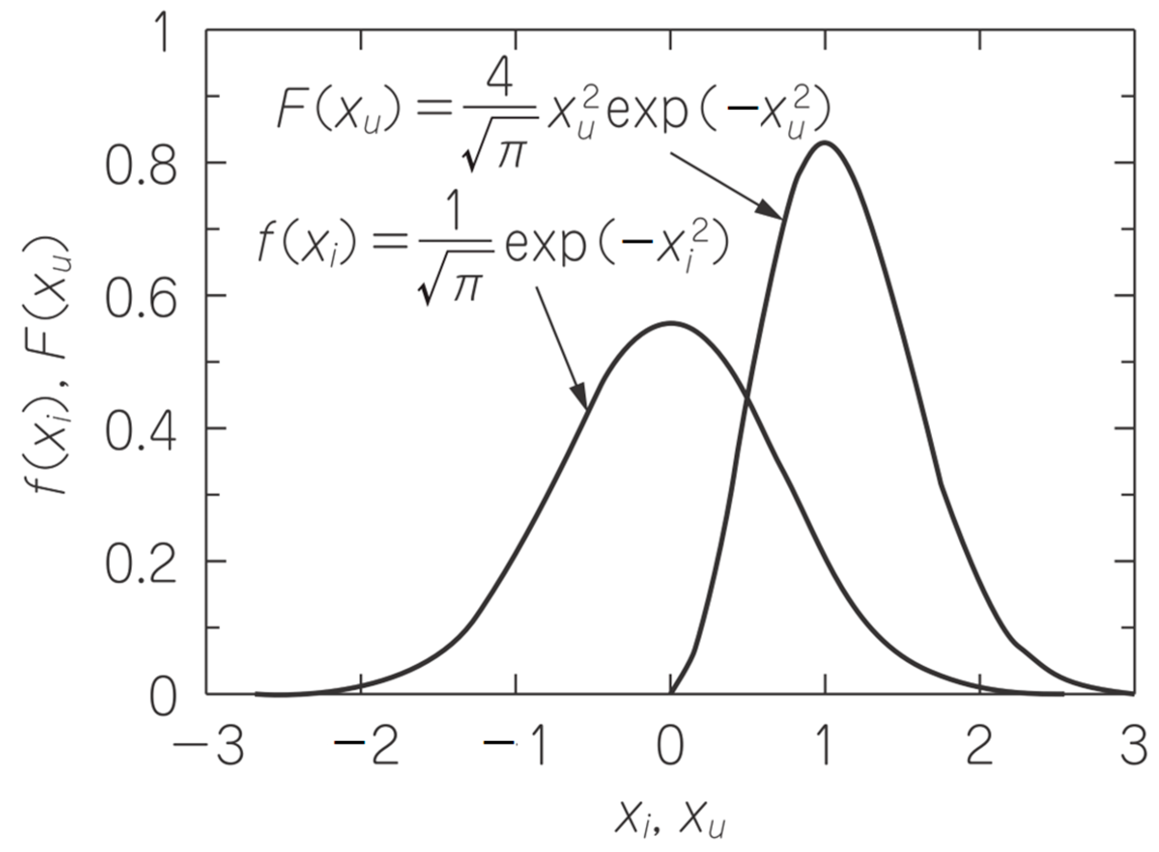
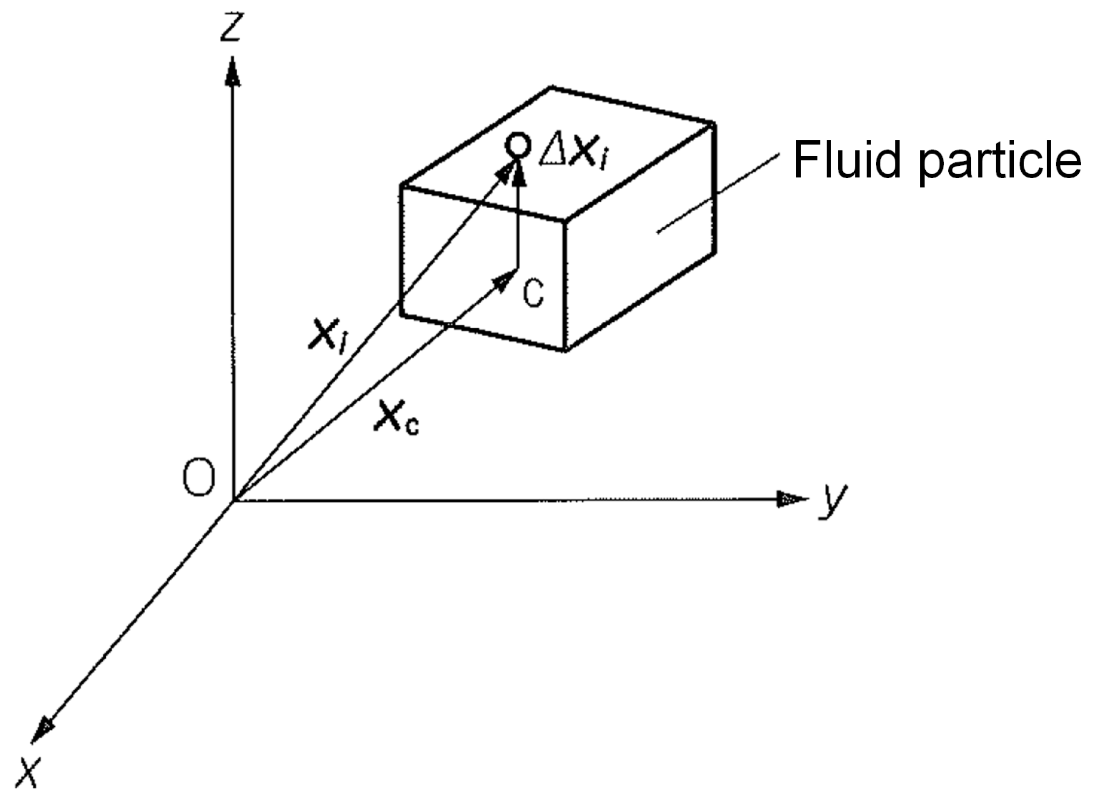
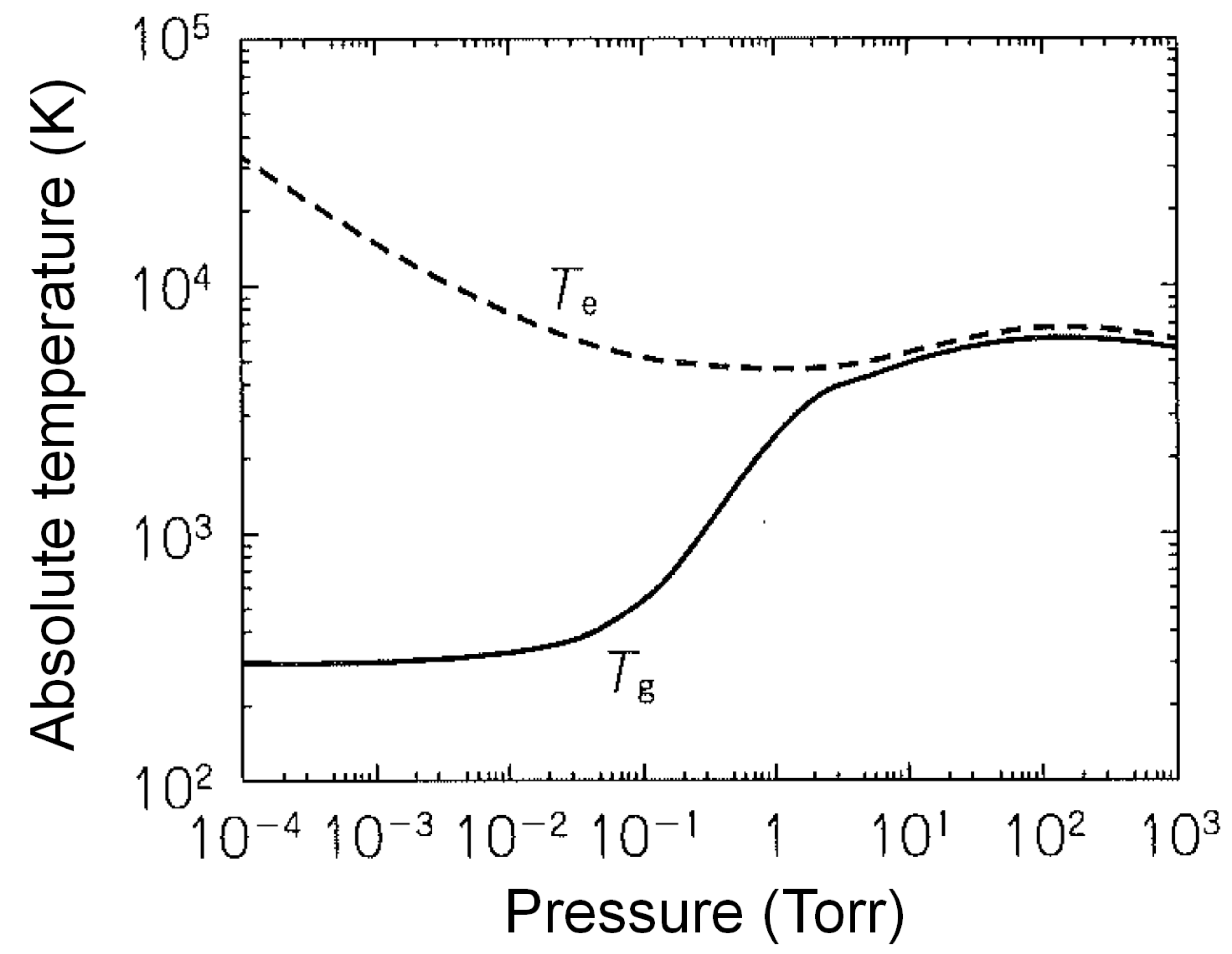
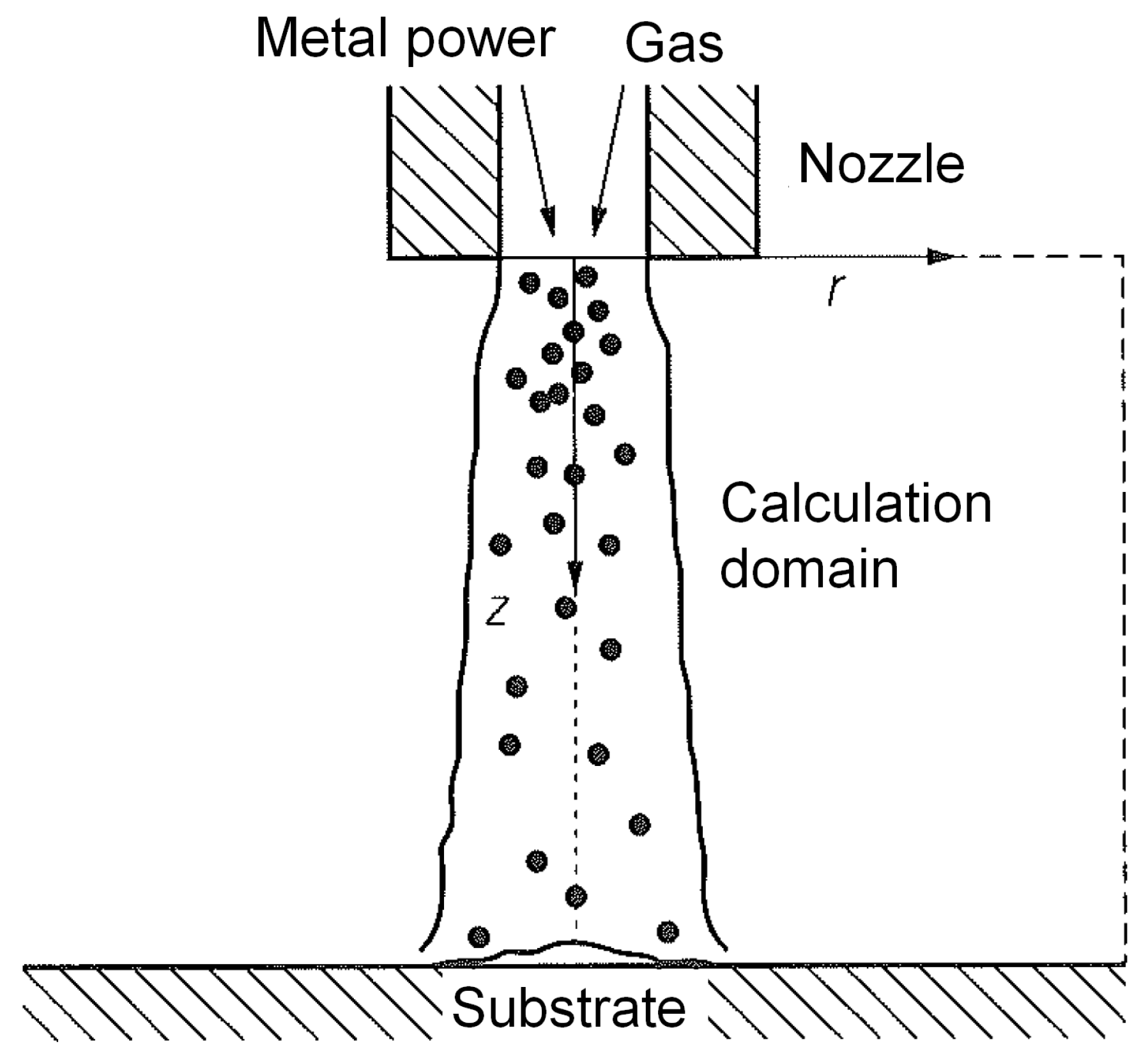
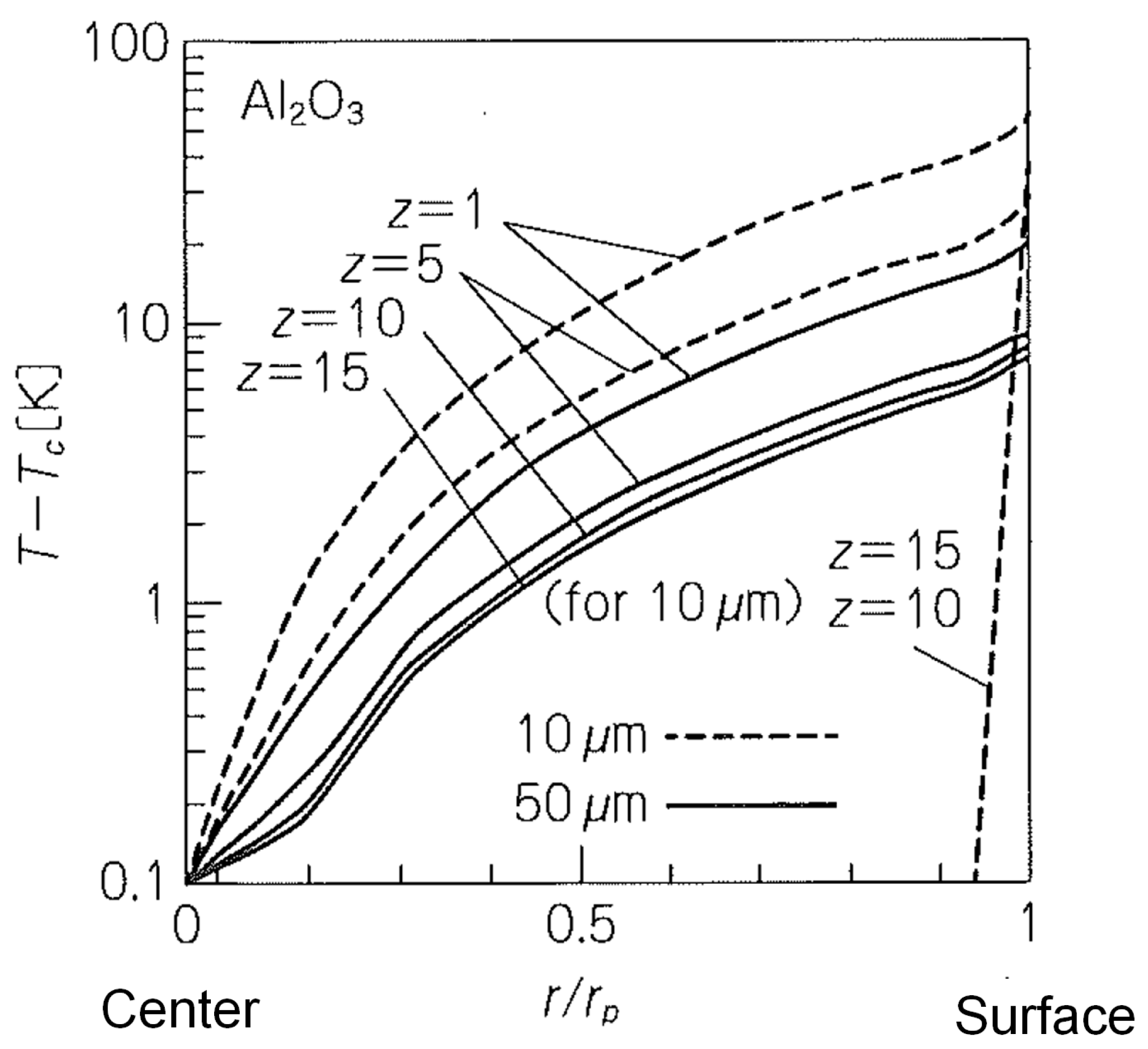
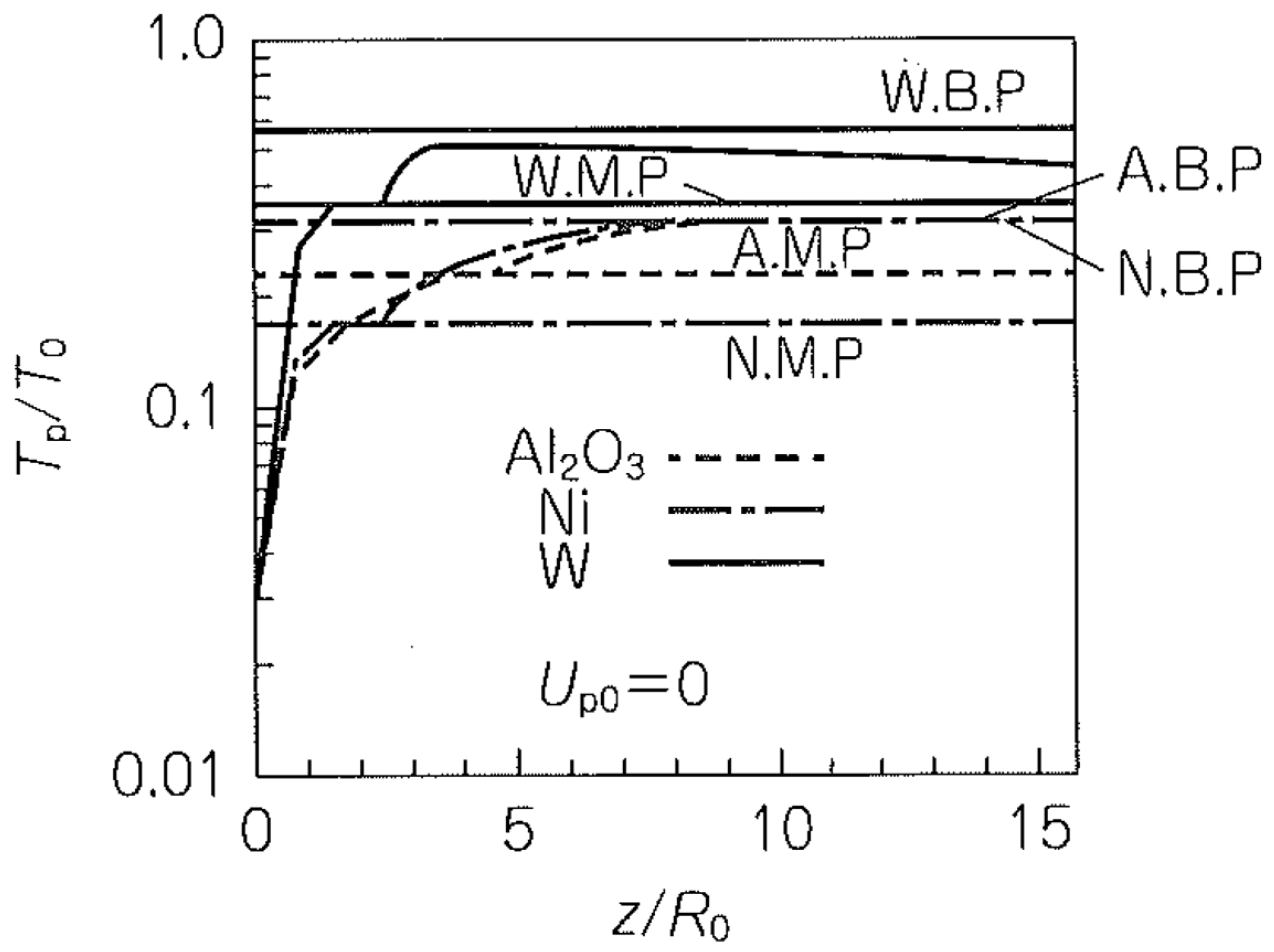
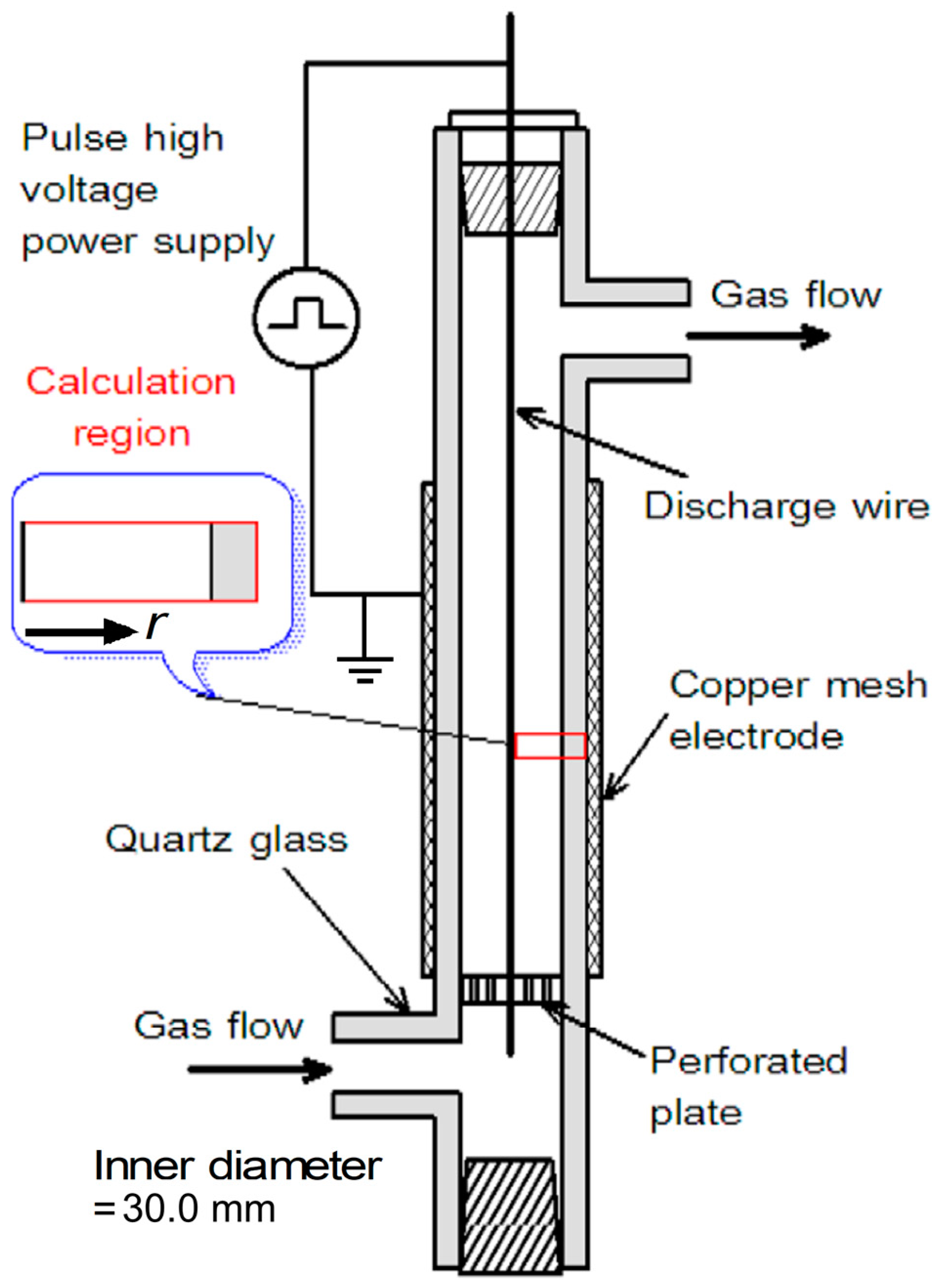
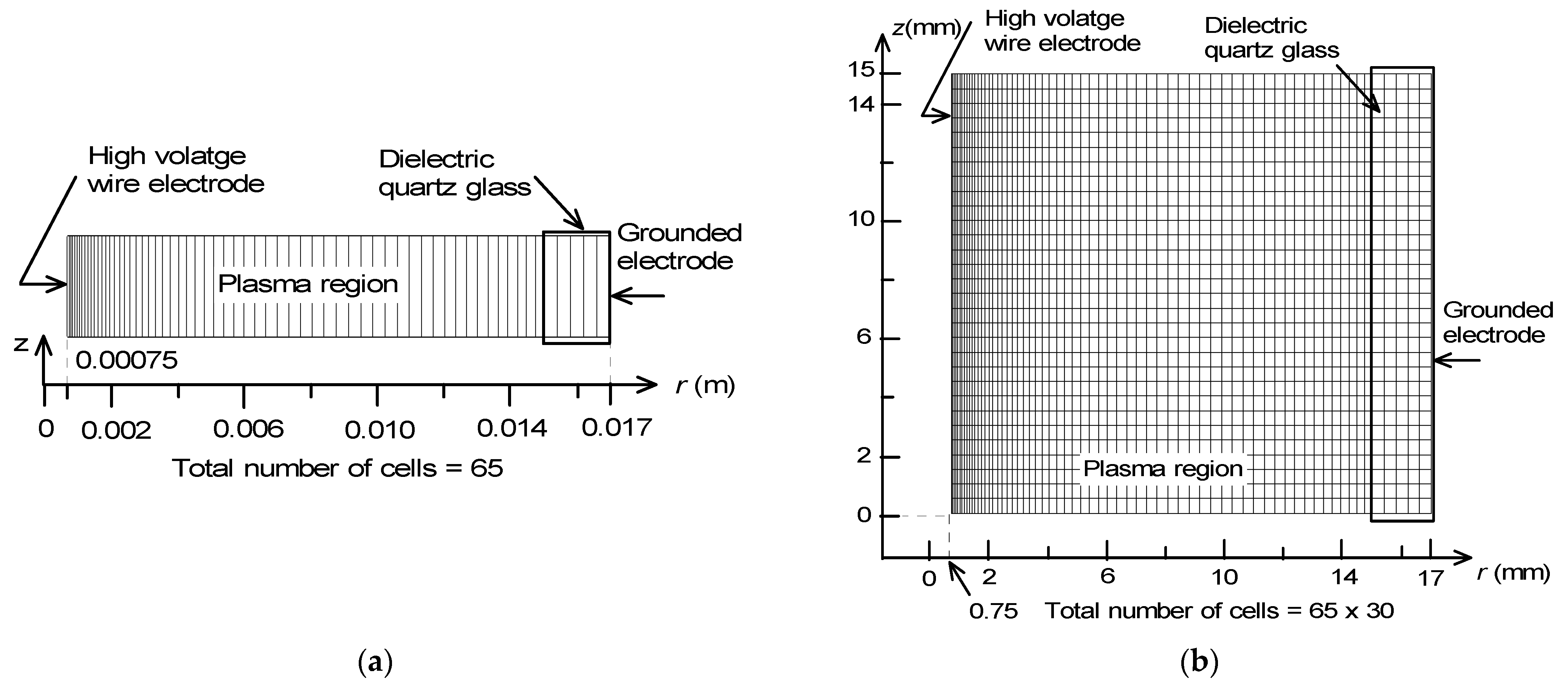
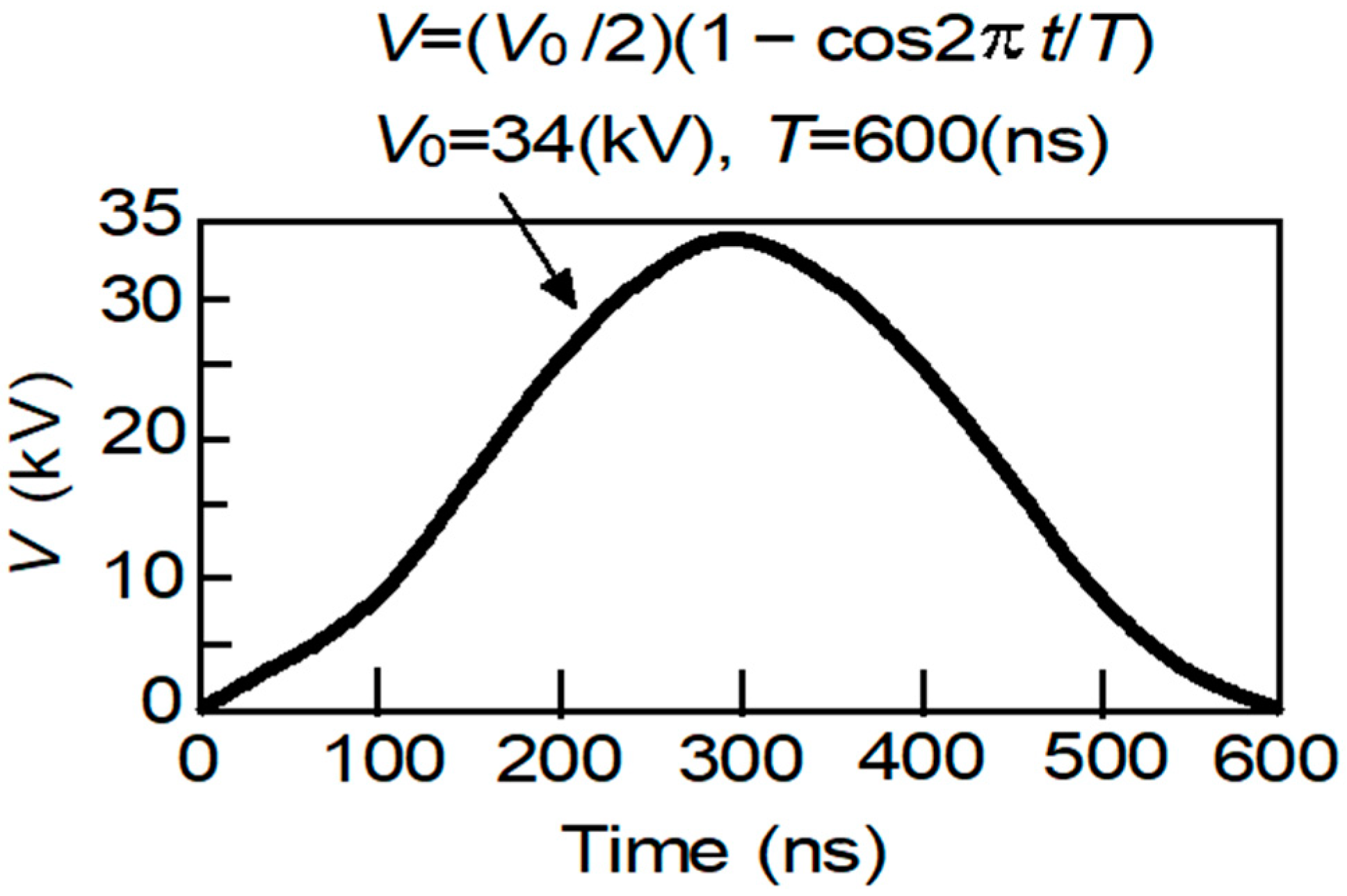
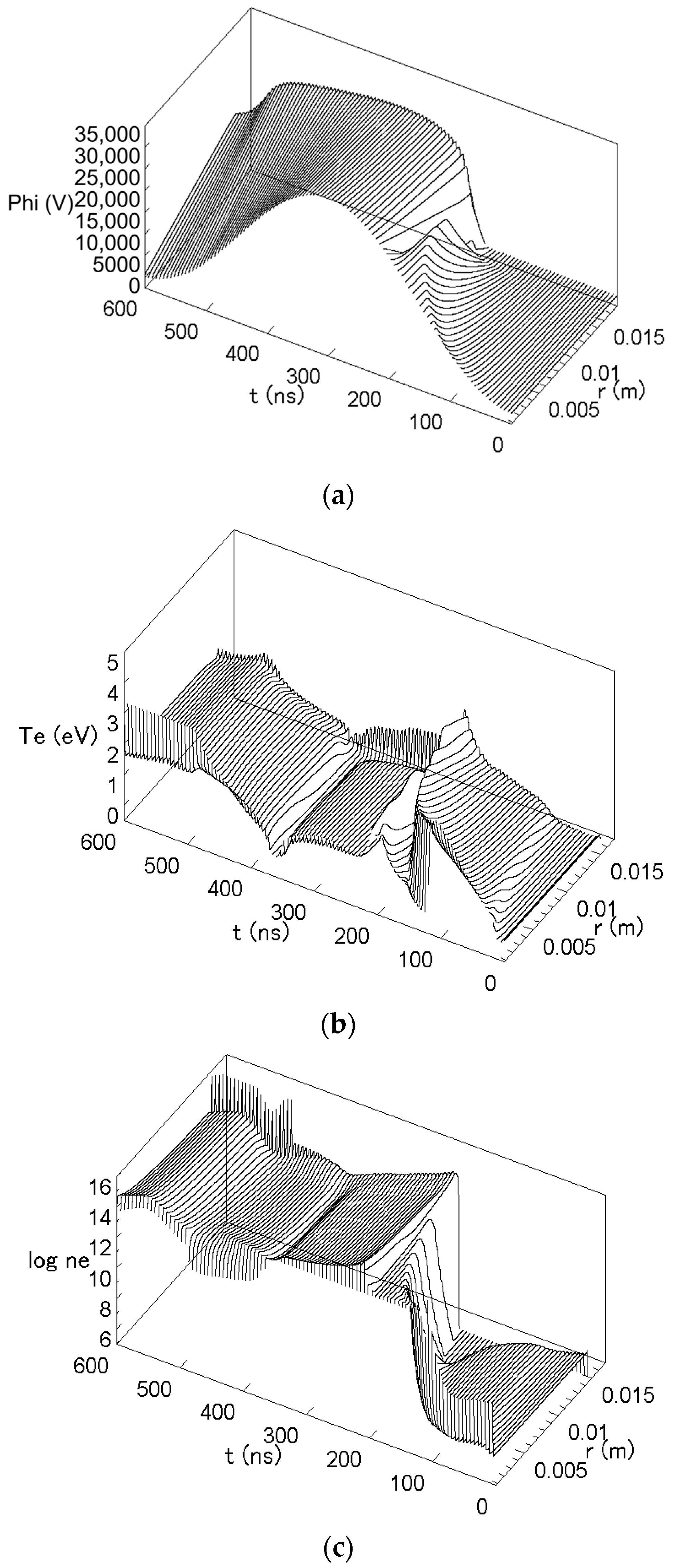
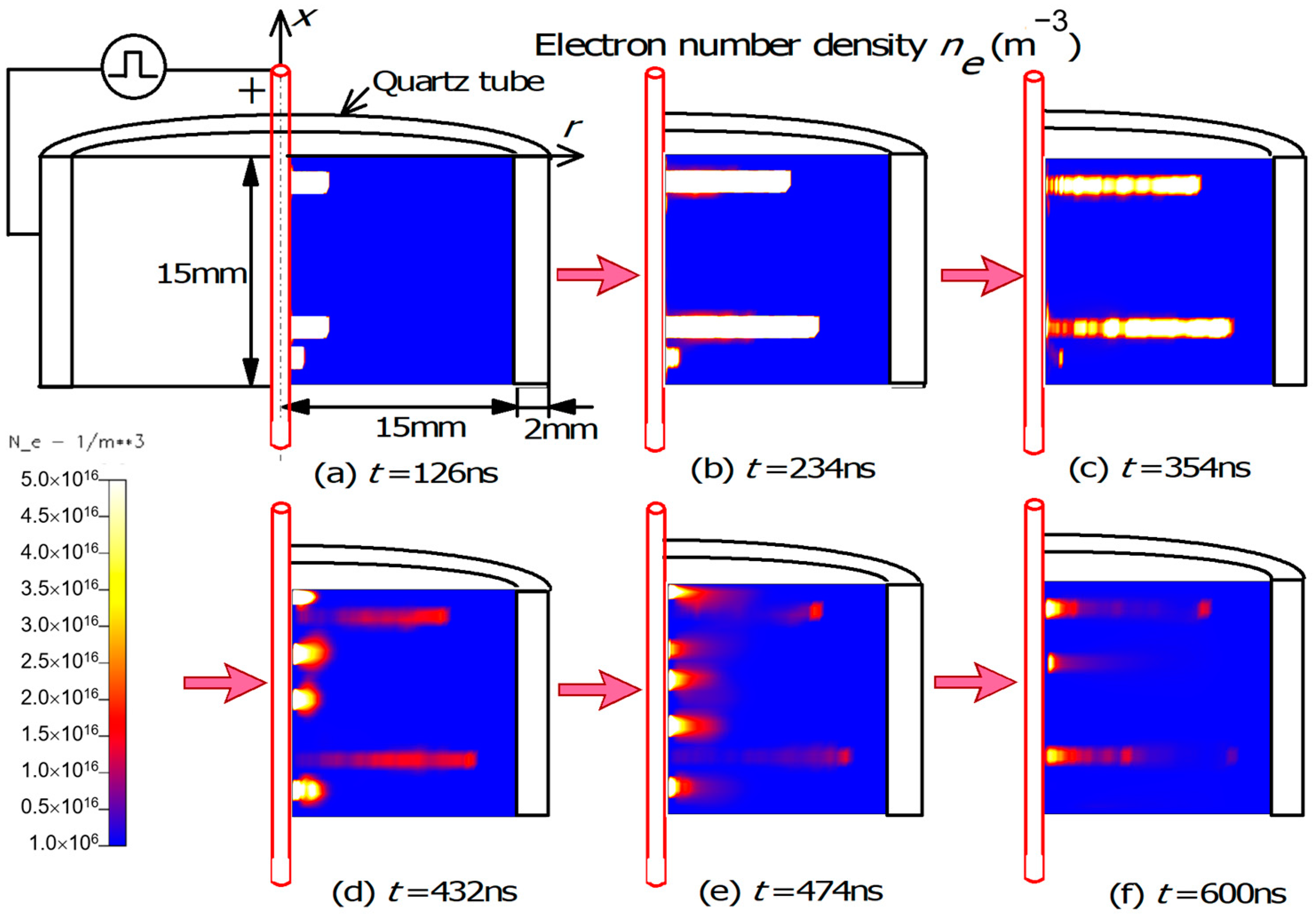
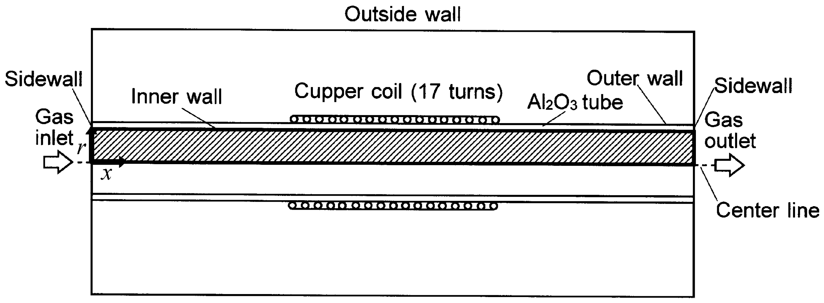
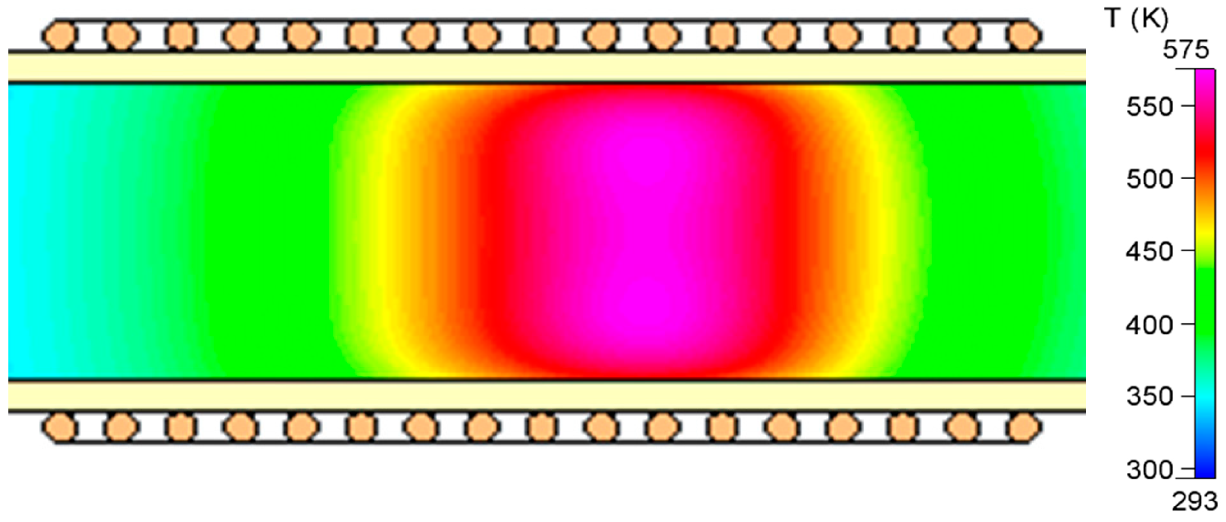
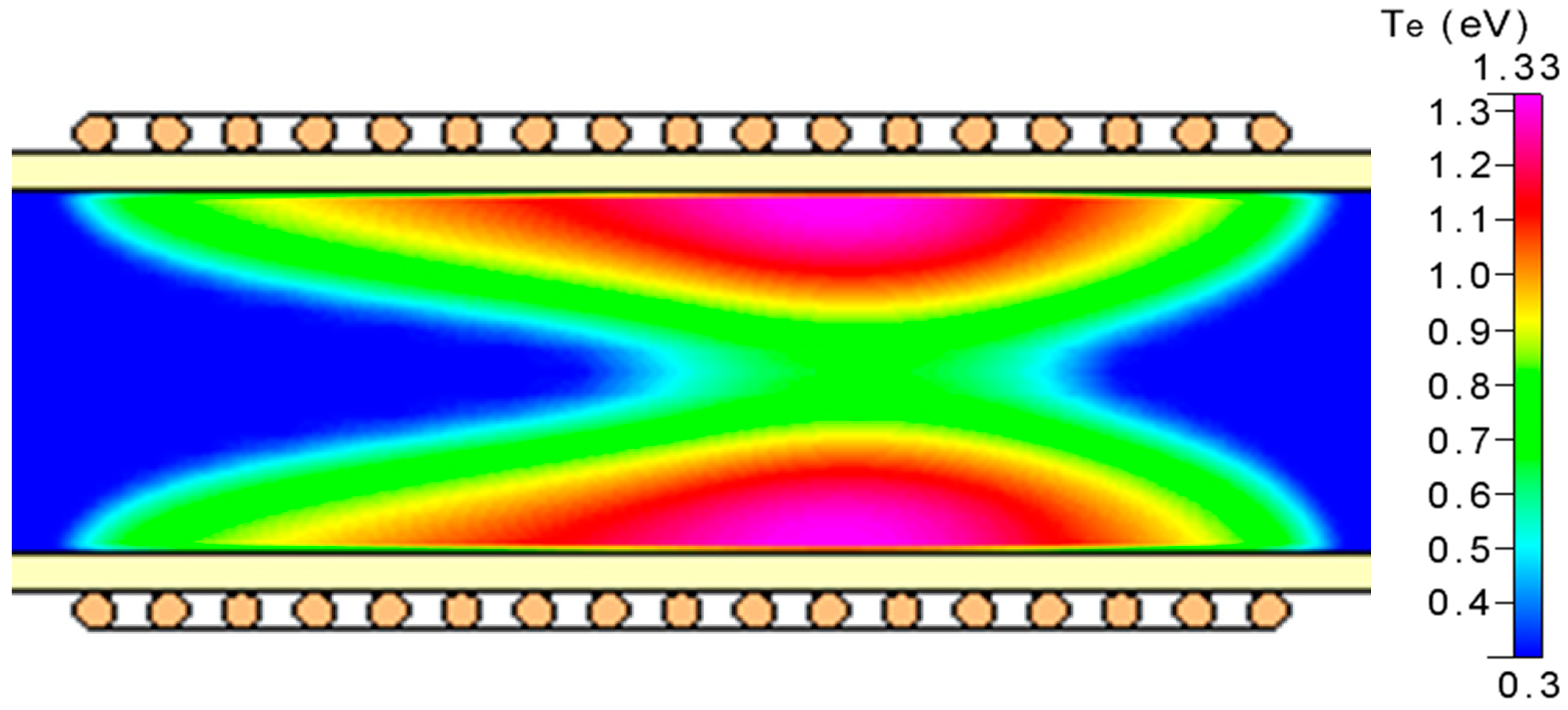
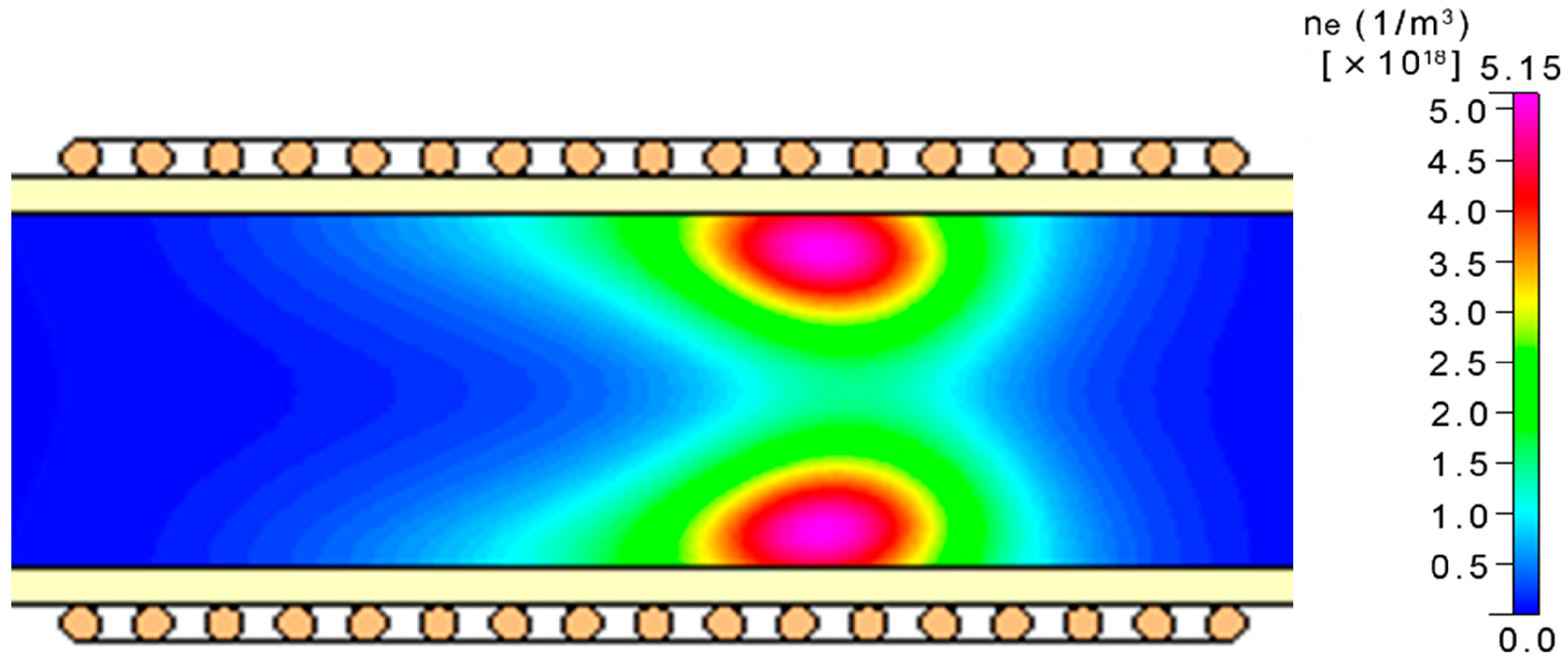
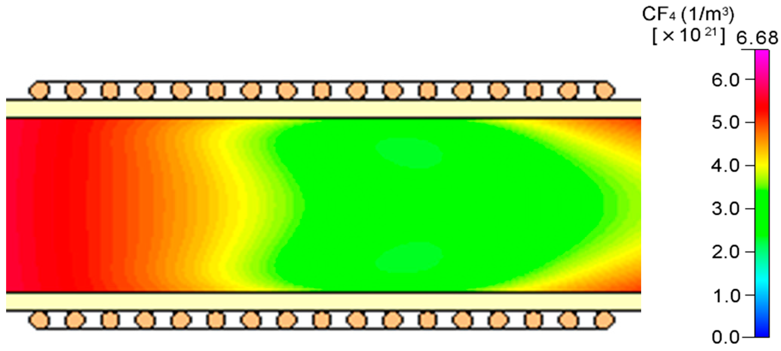
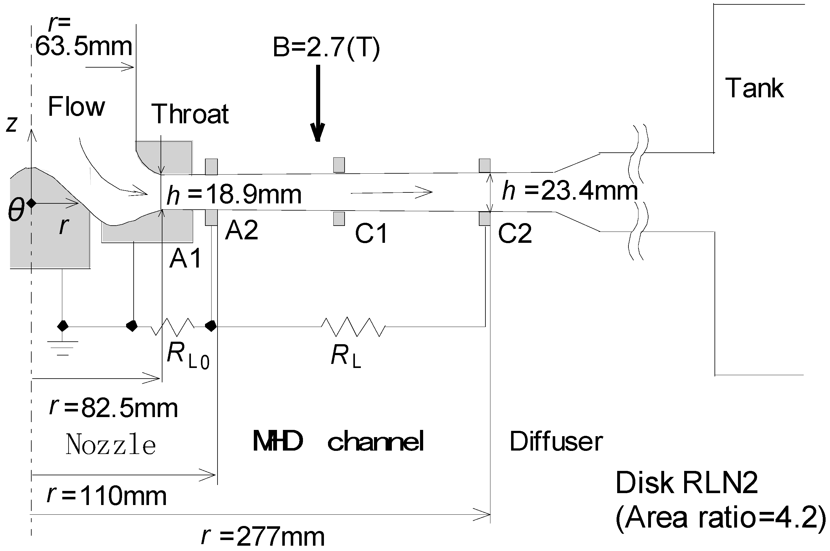
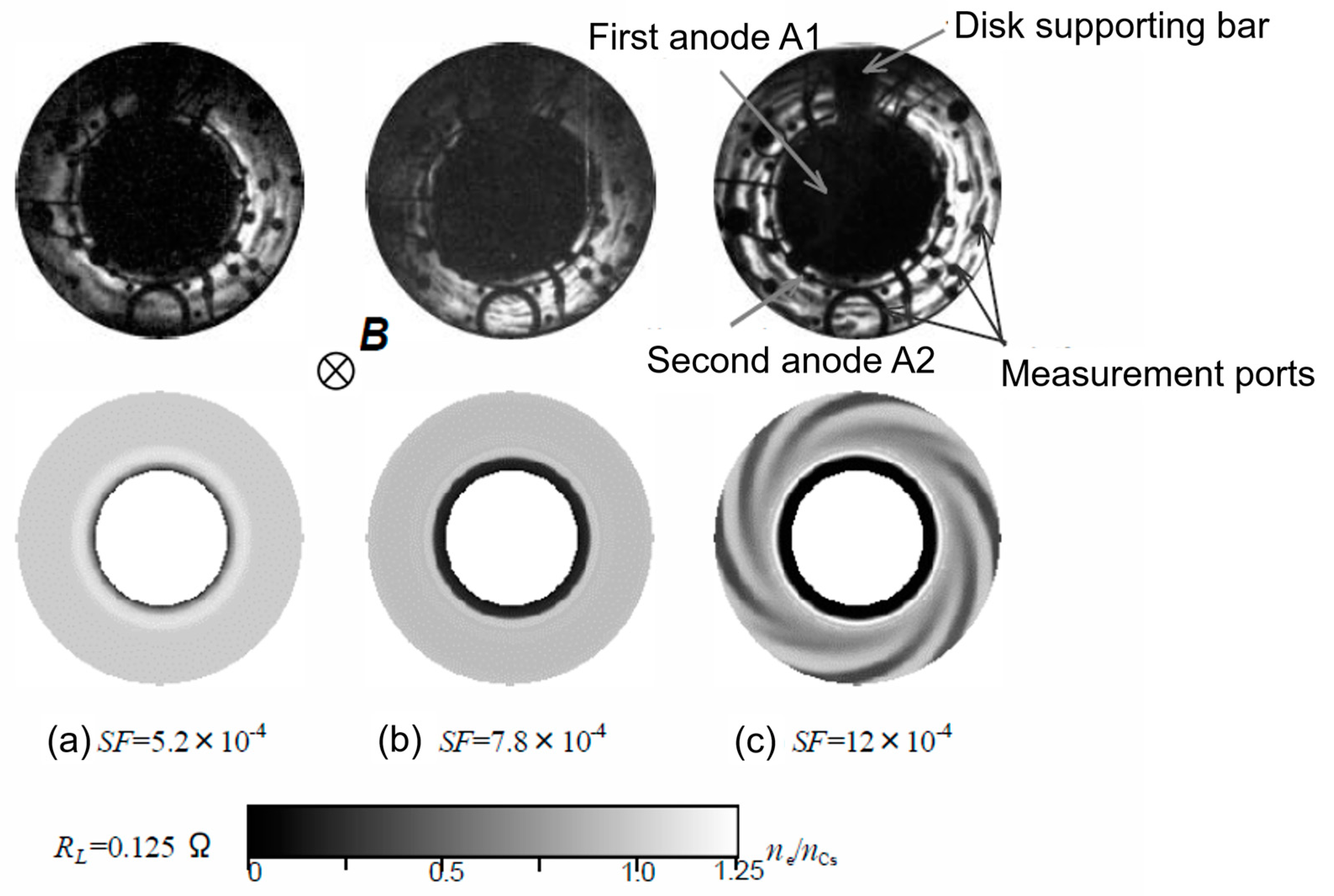
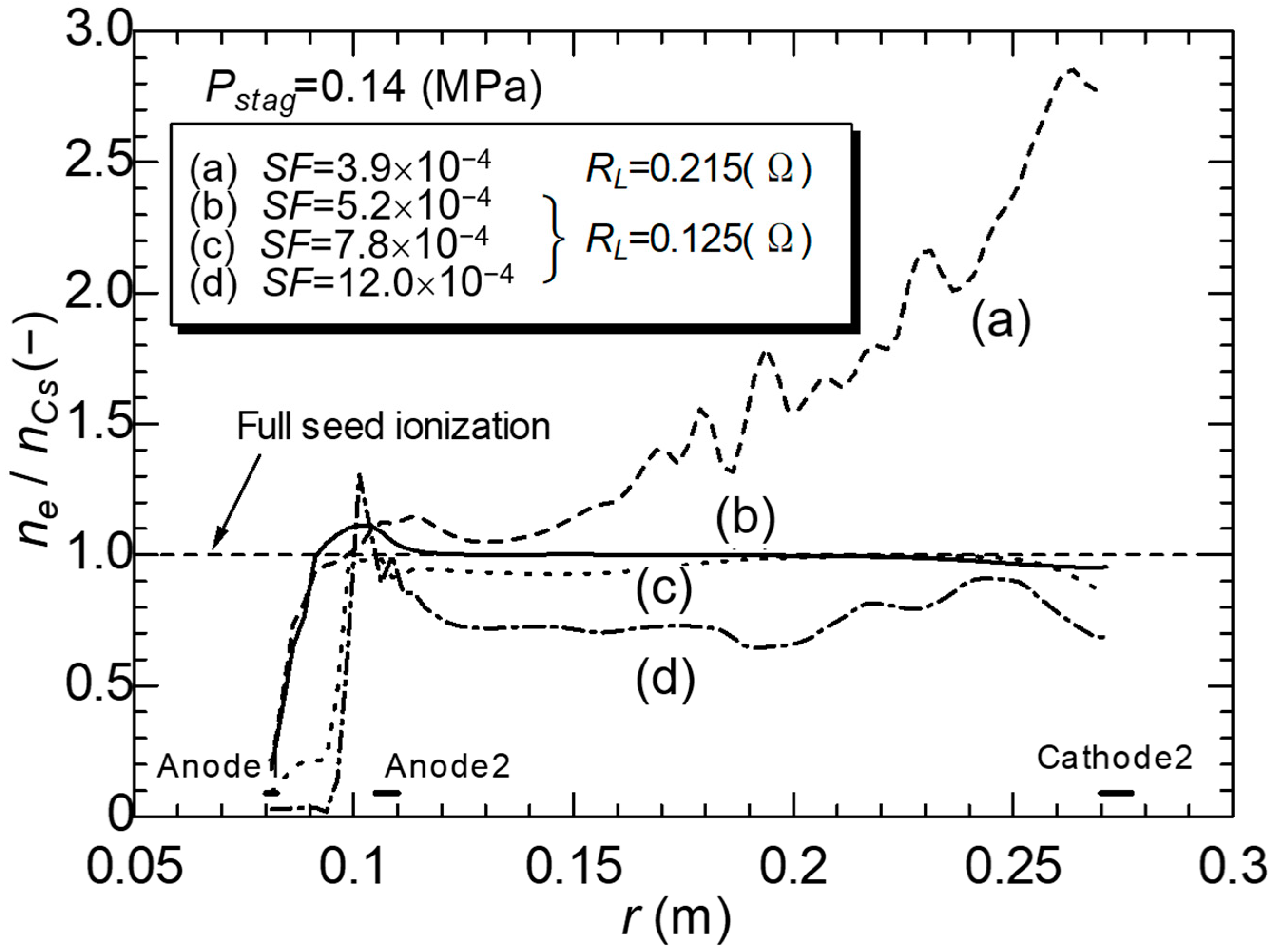
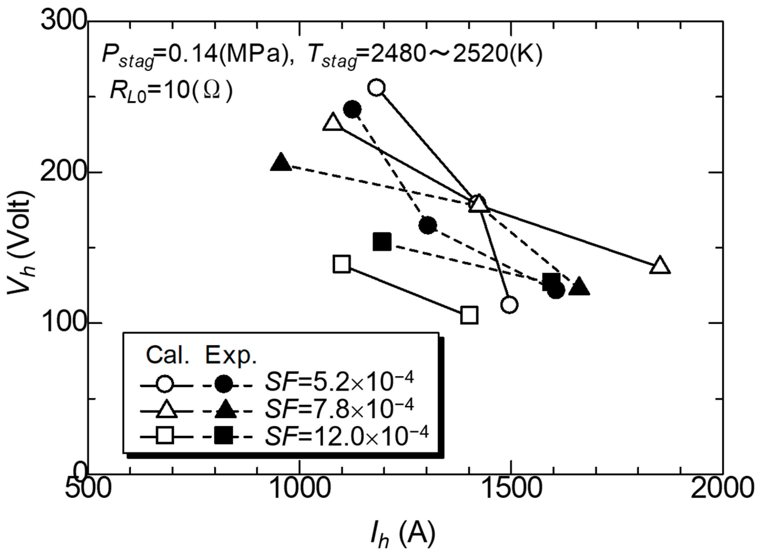
Table 1.
Calculation conditions (CF4 decomposition) [28].
Table 1.
Calculation conditions (CF4 decomposition) [28].
| AC Voltage frequency, MHz | 2 | |
| Atmospheric temperature, K | 293 | |
| Absolute pressure, Pa | 80 | |
| Power, kW | 2.0 | |
| Mass flow rate of gas, g/s | 0.02107 | |
| Initial mass fraction of species | CF4 | 0.5789 |
| O2 | 0.42105 | |
Table 2.
Calculation conditions [29].
Table 2.
Calculation conditions [29].
| Working gas | Ar/Cs |
| Stagnation temperature, K | 2480–2520 |
| Stagnation pressure, MPa | 0.14 |
| Seed fraction | (3.9–12.0) × 10−4 |
| Ext. load resistance RL0, Ω | 10 |
| Ext. load resistance RL, Ω | 0.075–0.215 |
| Area ratio of channel | 4.2 |
| Magnetic flux density, T | 2.7 (r = 82.5 mm) 0.39 (r = 270 mm) |
Disclaimer/Publisher’s Note: The statements, opinions and data contained in all publications are solely those of the individual author(s) and contributor(s) and not of MDPI and/or the editor(s). MDPI and/or the editor(s) disclaim responsibility for any injury to people or property resulting from any ideas, methods, instructions or products referred to in the content. |
© 2023 by the author. Licensee MDPI, Basel, Switzerland. This article is an open access article distributed under the terms and conditions of the Creative Commons Attribution (CC BY) license (https://creativecommons.org/licenses/by/4.0/).
Share and Cite
MDPI and ACS Style
Okubo, M. Fundamentals and Applications of Nonthermal Plasma Fluid Flows: A Review. Plasma 2023, 6, 277-307. https://doi.org/10.3390/plasma6020020
AMA Style
Okubo M. Fundamentals and Applications of Nonthermal Plasma Fluid Flows: A Review. Plasma. 2023; 6(2):277-307. https://doi.org/10.3390/plasma6020020
Chicago/Turabian StyleOkubo, Masaaki. 2023. "Fundamentals and Applications of Nonthermal Plasma Fluid Flows: A Review" Plasma 6, no. 2: 277-307. https://doi.org/10.3390/plasma6020020