Article

3t2FTS: A Novel Feature Transform Strategy to Classify 3D MRI Voxels and Its Application on HGG/LGG Classification

by
Abdulsalam Hajmohamad
1 and
Hasan Koyuncu
2,*
1
Electrical & Electronics Engineering Department, Konya Technical University, Konya 42250, Türkiye
2
Electrical & Electronics Engineering Department, Faculty of Engineering and Natural Sciences, Konya Technical University, Konya 42250, Türkiye
*
Author to whom correspondence should be addressed.
Mach. Learn. Knowl. Extr. 2023, 5(2), 359-383; https://doi.org/10.3390/make5020022
Submission received: 1 March 2023 / Revised: 31 March 2023 / Accepted: 5 April 2023 / Published: 6 April 2023
(This article belongs to the Special Issue Machine Learning for Biomedical Data Processing)

Abstract

:
The distinction between high-grade glioma (HGG) and low-grade glioma (LGG) is generally performed with two-dimensional (2D) image analyses that constitute semi-automated tumor classification. However, a fully automated computer-aided diagnosis (CAD) can only be realized using an adaptive classification framework based on three-dimensional (3D) segmented tumors. In this paper, we handle the classification section of a fully automated CAD related to the aforementioned requirement. For this purpose, a 3D to 2D feature transform strategy (3t2FTS) is presented operating first-order statistics (FOS) in order to form the input data by considering every phase (T1, T2, T1c, and FLAIR) of information on 3D magnetic resonance imaging (3D MRI). Herein, the main aim is the transformation of 3D data analyses into 2D data analyses so as to applicate the information to be fed to the efficient deep learning methods. In other words, 2D identification (2D-ID) of 3D voxels is produced. In our experiments, eight transfer learning models (DenseNet201, InceptionResNetV2, InceptionV3, ResNet50, ResNet101, SqueezeNet, VGG19, and Xception) were evaluated to reveal the appropriate one for the output of 3t2FTS and to design the proposed framework categorizing the 210 HGG–75 LGG instances in the BraTS 2017/2018 challenge dataset. The hyperparameters of the models were examined in a comprehensive manner to reveal the highest performance of the models to be reached. In our trails, two-fold cross-validation was considered as the test method to assess system performance. Consequently, the highest performance was observed with the framework including the 3t2FTS and ResNet50 models by achieving 80% classification accuracy for the 3D-based classification of brain tumors.

1. Introduction

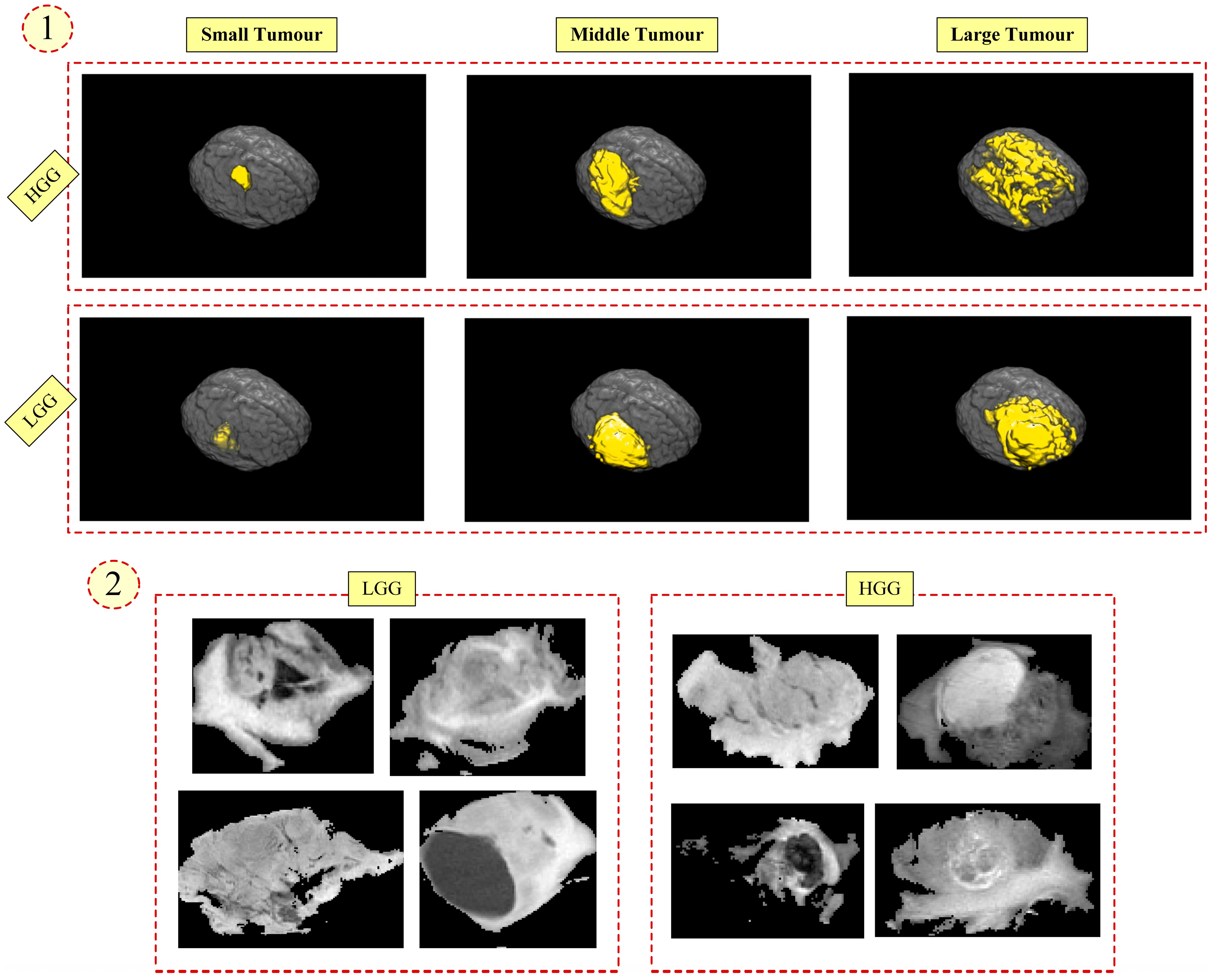
Glioma is the most frequent and one of the fastest growing brain tumors according to the grading system of the World Health Organization (WHO). Regarding this assessment, glioma is divided into four groups that are degree-I (pilocytic astrocytoma), degree-II (low-grade glioma), degree-III (malign glioma), and degree-IV (glioblastoma multiforme). Herein, the distinction of these tumors as high-grade glioma (HGG) and low-grade glioma (LGG) provides a significant opportunity to arrange treatment procedures and to make an estimation of the survival time of patients [1,2]. The survival time of patients with HGG-type tumors is almost two years, and this type of glioma requires rapid intervention. In contrast with HGG-type tumors, the growth rate of LGG-type tumors stays at low levels, and the survival time of patients with LGG can be kept as long as possible [3].
Magnetic resonance imaging (MRI) is often preferred to detect brain tumors in terms of revealing different abnormalities in tissue examinations [4]. In other words, MRI comes to the forefront on account of identifying even small tissue changes in comparison with the other imaging modalities [5]. However, the exploration of MRI slices involving both necessary information (tumor region) and irrelevant information (non-tumor region) can make the detection process hard. Regarding this, a computer-aided diagnosis (CAD) system can help medical experts, especially radiologists, to adjust the therapeutic initiatives [4].
In the literature studies, brain-based analyses (segmentation, classification, etc.) are handled and examined many times by using 2D- or 3D-based evaluations [6,7,8,9,10,11,12]. However, the accurate classification of brain tumors is evaluated less than the segmentation issue. At this stage, the classification process is nearly always realized using two-dimensional (2D) analyses instead of three-dimensional (3D) examinations of tumors.
Latif et al. [1] offered a system operating all phase information (T1, T2, T1c, and FLAIR), discrete wavelet transform (DWT), first- and second-order statistics, and multilayer perceptron (MLP) so as to perform the classification of tumor vs. non-tumor samples in 2D MRI images (BraTS 2015). In analyses, 39 HGG/26 LGG instances were utilized for training, and 110 HGG/LGG samples were considered for testing. In other words, a training-test split was considered to evaluate the system. Consequently, the proposed system achieved 96.73% accuracy and 99.3% AUC scores for the 2D-based classification of tumor availability. However, all training samples of BraTS 2015 were not considered in the study, and the semi-automated system was not appropriate to work with a segmentation method. Kumar et al. [2] presented a model including stationary wavelet transform (SWT), textural features including first-order statistics (FOS), recursive feature elimination (RFE), and random forest (RF) in order to classify the HGG vs. LGG samples in 2D MRI images (BraTS 2017/2018). In the experiments, all phase information was utilized, and five-fold cross validation was chosen to evaluate the performance. As a result, the proposed model attained 97.54% accuracy and 97.48% AUC scores for the 2D-based classification of brain tumors. However, the whole brain and region of interest (ROI) including the tumor area were utilized together for feature extraction, meaning that the proposed model constituted a semi-automated classification structure requiring both the choice of slice and ROI. In other words, the proposed model was functional with a 2D-based segmentation algorithm and with an expert to choose the slice. Saba et al. [3] designed a framework involving histogram orientation gradient (HOG), local binary patterns (LBP), deep features, and a classifier so as to discriminate 2D images that are labeled as HGG vs. LGG and as normal vs. tumor. In trials, a 50%-50% training-test split was preferred as the test method, and ensemble classifier (EC) was the best algorithm on average classification performance for three datasets. The proposed framework obtained accuracies of 91.30%, 91.47%, and 98.39% on the BraTS 2015, BraTS 2016, and BraTS 2017 datasets, respectively. Moreover, the framework was proposed as a semi-automated algorithm concerning slice selection. Gupta et al. [4] proposed a three-level classification system utilizing a T2 + FLAIR phase combination, morphological operations, inherent characteristics, and majority voting-based EC for HGG vs. LGG categorization. Moreover, the proposed system included a T2 + FLAIR phase combination, grey level co-occurrence matrix (GLCM), grey level run length matrix (GLRLM), LBP, and majority voting-based EC for normal vs. tumor discrimination. In the experiments, two datasets containing BraTS 2012 were used, and ten-fold cross-validation was considered for evaluation. Consequently, an average accuracy of 96.75% was observed in the HGG vs. LGG classification of 2D MRI images by the system presenting a semi-automated structure. Sharif et al. [5] suggested a pipeline comprising a T2 + FLAIR phase combination, HOG, LBP, geometric features, and support vector machines (SVM) for the categorization of healthy vs. unhealthy samples in 2D MRI images. To evaluate the pipeline, three datasets involving BraTS 2013 and BraTS 2015 were handled, and a 50%-50% training-test split was chosen as the test method. The suggested pipeline acquired 98% and 100% accuracy scores for the BraTS 2013 and 2015 datasets, respectively. Consequently, a semi-automated pipeline achieving promising scores was presented to the literature for 2D-based classification of healthy vs. unhealthy images. Bodapati et al. [13] presented a two-channel classification model based on deep neural network (DNN) algorithms: InceptionResNetV2 and Xception. To fulfill the performance assessment, five-fold cross-validation was preferred, and two datasets including BraTS 2018 were considered. According to the results, it was revealed that the proposed two-channel DNN outperformed other deep learning approaches by attaining 93.69% accuracy on the BraTS 2018 dataset. In [13], the input data of the model was defined as 2D MRI images, meaning that the operating condition of the model was proposed on a semi-automated basis. Koyuncu et al. [14] proposed a detailed framework handling a T1 + T2 + FLAIR phase combination, FOS features, Wilcoxon feature ranking, and an optimized classifier named GM-CPSO-NN for discrimination of HGG/LGG samples in 3D MRI images. In experiments, two-fold cross-validation was considered to assess the performance, and the BraTS 2017/2018 dataset was considered to perform the classification. As a result, the proposed framework obtained 90.18% accuracy and 85.62% AUC scores for the 3D-based classification of brain tumors.
Concerning the literature results, it can be seen that 3D-based classification reveals a more complicated issue in comparison with 2D-based classification due to the success scores and the information amount to be processed. In addition, 3D-based information requires comprehensive analyses to accurately perform the classification task. Beyond this, a fully-automated CAD system classifying the degree of brain tumors independently with the help of an expert can only be realized using the 3D tumor obtained from a segmentation method. Herein, the motivation of this paper arises which is the design of a model handling the 3D-based classification of HGG/LGG data in 3D MRI images. This paper is formed considering the requirements stated in the literature and contributes to the literature on the following subjects:
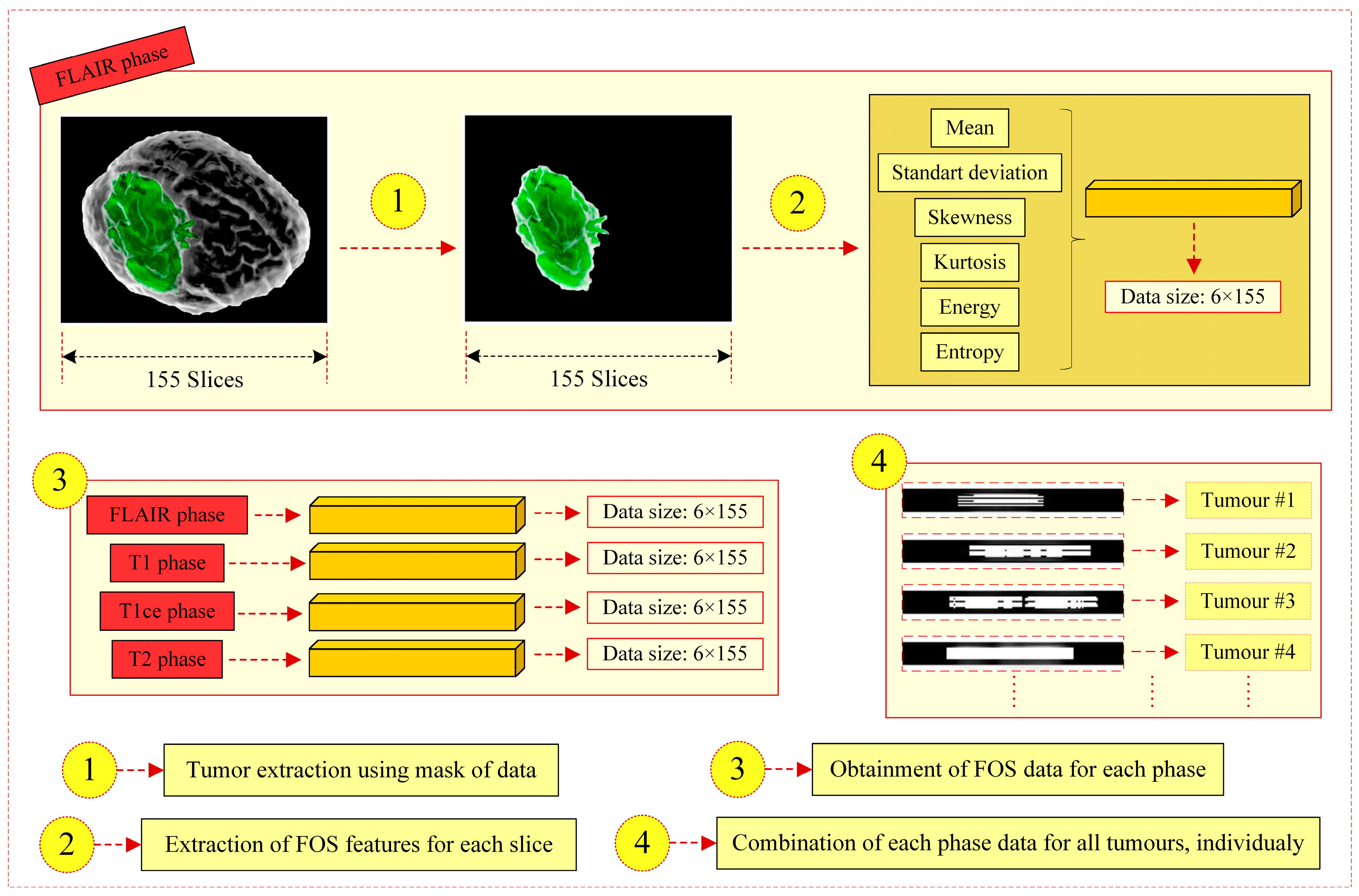
  • A novel 3D to 2D feature transform strategy (3t2FTS) that can be utilized to classify tumors in 3D MRI images;
  • A detailed application analyzing the information of a 3D voxel by transforming the space from 3D to 2D;
  • A comprehensive study considering the comparison of eight qualified transfer learning architectures on tumor grading;
  • An efficient framework to be determined for guiding 3D MRI-based classification tasks.
The organization of this paper is as follows. Section 2 briefly explains the utilized FOS features in-depth, describes the proposed 3D to 2D feature transform strategy, gives the dataset information with its handicaps, and briefly declares the transfer learning algorithms. Section 3 presents the experimental analyses and interpretations of the comparison of transfer learning methods for two-fold cross-validation-based evaluations. Section 4 reveals the discussions about the results extracted. The concluding remarks are given in Section 5.

2. Materials and Methods

2.1. First-Order Statistics

First-order statistics (FOS) are generated using the histogram-based intensity analyses of an image. Concerning the histogram evaluations, six phenomena (mean, standard deviation, skewness, kurtosis, energy, and entropy) constitute the most preferred FOS features in the literature [14,15,16,17].
Let the f(x,y) function symbolize the 2D image. At this point, the ‘x’ and ‘y’ variables are defined as the coordinates of the image in horizontal and vertical planes, respectively, and these are respectively specified as (x = 0, 1, …, X − 1) and (y = 0, 1, …, Y − 1). Herein, let G be the total intensity number of the image. Then, a discrete intensity value ‘i’ or the output of the function f(x,y) can own values in the range of [0, G − 1] which shows the values of intensity levels. Hereupon, the histogram arises as a statistical assessment of the repetition number of intensity levels among the image [14,15,16,17].
The size of an image is described in width and height, and the number of slices is taken into consideration to define the 3D space. Let W, L, and N signify the width, length, and number of slices, respectively. After this, the total voxel number of volume of interest (VOI) is obtained by multiplying the width ‘W’, length ‘L’, and slice number ‘N’. In relation to this, h(i) and Kronecker delta function can be identified as in (1) and (2) [14,15,16,17].
h ( i ) = x = 0 L 1 y = 0 W 1 δ ( f ( x , y ) , i )
δ ( j , i ) = 1 , j = i 0 , j i
To obtain the probability density function (PDF) of intensity ‘i’, the value of ‘h(i)’ is divided by the total voxel number of the VOI as in (3) [14,15,16,17].
p ( i ) = h ( i ) 1 × N × W × L , i = 0 , 1 , 2 , 3 . , G 1
By utilizing the PDF values, the FOS features of the VOI can be quantitatively calculated as the mean, standard deviation, skewness, kurtosis, energy, and entropy which are respectively indicated in (4–9) [14,15,16,17].
μ = i = 0 G 1 i p ( i )
σ = i = 0 G 1 ( i μ ) 2 p ( i )
μ 3 = σ 3 i = 0 G 1 ( i μ ) 3 p ( i )
μ 4 = σ 4 i = 0 G 1 ( i μ ) 4 p ( i ) 3
E n e r g y = i = 0 G 1 p ( i ) 2
E n t r o p y = i = 0 G 1 p ( i ) log 2 p ( i )

2.2. 3D to 2D Feature Transform Strategy

In 2D-slice-based analysis, voxel information of tumors is ignored which constitutes the most significant part of a fully automated CAD system. The proposed 3D to 2D feature transform strategy (3t2FTS) aims to define the 3D information in 2D space by using FOS features. The utilized FOS features are arranged as the mean, standard deviation, skewness, kurtosis, energy, and entropy. At this point, we want to produce 2D identification (2D-ID) images of 3D tumors by examining all slices and all MRI modalities. In other words, as a result of the transformation, a 2D-ID image responding to the characteristic of the tumor is proposed to be generated. Herein, all phase combinations (T1, T2, T1c, and FLAIR) were examined concerning the literature advice since every phase can involve different information belonging to different kinds of tumors [1,2,14]. Regarding this, Figure 1 presents the design of 3t2FTS and can be interpreted as follows:
  • The tumor is obtained in 3D via a segmentation method or a 3D mask of the utilized dataset. In this paper, the mask of data is chosen, and the classification process is focused on.
  • FOS features are evaluated at each slice in the 3D image. In this study, the slice number is 155, and a matrix at the size of 6 × 155 is acquired for one phase of MRI.
  • The second process is performed for all phases or MRI modalities.
  • All phase information is combined, and for one tumor, a 2D-ID image is obtained of which the size is ‘(FOS feature number × the utilized modality number) × slice number’.
A 3D tumor can be identified as a 2D-ID image as a result of the 3t2FTS approach, and the size of the 2D-ID image is revealed as 24 × 155 for our study according to the parameter values defined in item 4. Moreover, the 3t2FTS approach can easily be adapted for different kinds of tumors handled in 3D MRI too, since it directly evaluates the tumors in 3D and extracts the necessary information to the 2D space.

2.3. Dataset Information and Handicaps

The BraTS 2017/2018 dataset involves 210 HGG and 75 LGG instances in 3D MRI images for training. In every 3D sample, the slice number is 155, and every slice is defined in 3D regarding the RGB space. The dataset comprises four imaging modalities that are T1, T2, T1c, and FLAIR phases. Concerning the modalities and slice number, 620 slices are considered for tumor analysis of one patient. The image size and thickness of a slice are 240 × 240 and 1mm, respectively [18,19,20].
In the training dataset, there exists a mask to reveal the tumor regions which are categorized as GD-enhancing (label 4), peritumoral (label 2), non-enhancing and edema (label 1), and background (label 0). In our paper, the tumor region is extracted using a mask (the first step of Figure 1) by assigning labels 1-2-4 as ‘1’ and label 0 as ‘0’. Herein, we have considered all tumor regions together since a segmentation method extracting sub-regions or the whole tumor should be combined with our proposed model [18,19,20]. Figure 2 visually presents the handicaps of the dataset [14].
In Figure 2, the first presentation (item 1) is concerned with the shape and size analyses of tumors. If a detailed examination is made in horizontal perspective for item 1, it can be observed that an LGG or HGG tumor can have very different shape and size characteristics even in the same category. In contrast, HGG- and LGG-type tumors can have similar shape and size features if the examination is made from a vertical perspective. In other words, distinct information about shape and size is not available for the tumor classification of HGG and LGG labels.
In Figure 2, the second presentation (item 2) is related to the intensity evaluation of HGG- and LGG-type tumors. Herein, it can be seen that the intensity level of a tumor can vary so much in the same category or can be similar for different categories. In other words, a distinguishing characteristic is not visually available to discriminate the HGG- vs. LGG-type tumors.
Concerning the handicaps, the comprehensive analyses of attribute extraction and robust classifier selection arise as the most significant issues in effectively assigning the class labels. Furthermore, the challenge of the 3D-based classification of brain tumors (item 1 and item 2) comes to the forefront in comparison with the 2D-based classification task (item 2), since the necessary information identifying 3D tumors should be found. In addition, robust classifiers should be chosen to perform accurate classification of different types of tumors.

2.4. Transfer Learning Methods

In this section, eight convolutional neural networks (CNNs) are presented, and the visual representations of models involve dropout (layer elimination ratio), fully connected, or both blocks, meaning that these blocks symbolize the operation of NNs.

2.4.1. DenseNet201 Architecture

DenseNet201 is an efficient version of dense connected convolutional networks (DenseNet) generated on the basis of the feed-forward operating concept [21]. DenseNet eases the vanishing gradient problem, and it enables the reuse of input data at the next layers by improving feature propagation. Herein, DenseNet is generated on the basis of dense blocks in which the feature map generated in previous layers seems significant to be fed as the input to the next layers on upgrading the system recognition of input data. In brief, it is declared that DenseNet-based models consider the reuse of features, utilization of short connections, and deeper model attainment for achieving better performance [21,22]. Figure 3 presents the architecture of the DenseNet201 model [21,22].
DenseNet201 utilizes convolution layers, dense blocks including multi-connected convolution layers, average and max pooling approaches, a fully connected layer, and the softmax function to evaluate the input image. In DenseNet201, transition layers involving convolution and average pooling are utilized to define the feature map having necessary decreased features fed to another dense block.

2.4.2. InceptionResNetV2 Architecture

InceptionResNetV2 rises as a hybrid model consisting of residual connections and inception phenomenon [23]. Inception networks using inception modules are handled to overcome the problems oriented from traditional CNNs, i.e., overfitting, low performance, etc. To ease the network structure and accelerate the decision process, the residual connection is effectively considered for the design of very deep networks. With the combination of two concepts, InceptionResNet-based models are produced [23,24].
InceptionResNetV2 operates a stem module, three InceptionResNet-based modules (InceptionResnet-A, InceptionResnet-B, and InceptionResnet-C), reduction modules (Reduction-A and Reduction-B), average pooling, dropout, and the softmax function. Figure 4 and Figure 5 present the architecture of InceptionResNetV2 and the modules of the model, respectively [23,24].
InceptionResNetV2 utilizes filter concatenation (filter concat or concat) to stack different data with various sizes. In other words, no information is missed among the layers in which concat is used to combine the various information provided. The stem module performs down-sampling in the input data to accelerate the workflow and reduces the memory usage and computational cost of the whole architecture. Three InceptionResNet-based modules consider multiple-sized kernels to decrease the computational complexity. Moreover, by using the residual concept, the input information is transformed and fed to the module output to merge more information. Moreover, residual flow improves the module output and acts as a bypass operator for situations in which necessary information cannot be propagated after training. Reduction modules aim to perform the dimensional reduction of data by preventing information loss [23,24].

2.4.3. InceptionV3 Architecture

InceptionV3 can be seen as an underdeveloped version of InceptionResNetV2 which is generated on the rationale of InceptionV3. The repeated residual blocks are compressed in InceptionResNetV2 according to InceptionV3 [25,26,27].
InceptionV3 employs three inception modules (Inception-A, Inception-B, and Inception-C), two reduction modules (Reduction-A and Reduction-B), average and max pooling approaches, dropout and fully connected NNs, and the softmax function. If a detailed examination is performed, it can be seen that InceptionV3 differs from InceptionResNetV2 when thinking about either the internal structure of the utilized blocks or the usage number of modules inside. Figure 6 presents the schematic view of the InceptionV3 model [25,26,27].
InceptionV3 reveals an improved version of InceptionV1 and InceptionV2 architectures so as to eliminate the computational costs and in order to upgrade performance by changing the convolutional kernel sizes in modules, applying asymmetric convolutions, and using axillary classifiers. The reduction of kernel sizes and the implementation of asymmetric convolutions instead of multiplying the data with a large kernel, stay as a qualified adjustment to decrease the computational costs. Moreover, the bottleneck layer including 1 × 1 kernels is also evaluated just before the main convolutions in order to reduce the parameter number. With the help of these concepts, InceptionV3 is produced deeper than the InceptionV1 and InceptionV2 models by not optimizing the time complexity. Herein, the axillary classifier which is the output of filter concatenation at the end of Inception-B is concerned with providing better convergence towards the end of the whole network. In other words, this concept encourages the usage of necessary gradients towards the network, whilst it tries to eliminate the vanishing gradient problem. Concerning this, axillary classifiers are notably preferred in recent inception-based CNNs [25,26,27].

2.4.4. ResNet50 and ResNet101 Architectures

The number of layers can upgrade the accuracy of the model. However, the deeper the networks, the more the accuracy of the model can degrade during the training process. Concerning this, ResNet-based models including ResNet50 and ResNet101, are proposed to eliminate the vanishing gradient problem in deeper networks. Figure 7 shows the design of ResNet50 and ResNet101 on the same schematic [28,29,30].
Both models (ResNet50 and ResNet101) operate five main convolutional blocks including convolutions with the same kernel size (Conv_1, …, Conv_5), average and max pooling approaches, fully connected NN, and the softmax function. Herein, the outstanding difference is the repetition of the Conv_4 block for both models.
Residual networks (ResNets) or other architectures involving ResNets, e.g., InceptionResNetV2, operate skip connections (residual connections) to keep the performance at high levels and to prevent information loss in deeper layers. In ResNet-based models, skip connections are evaluated to skip some layers and to feed the output of a layer to the next layers. Moreover,, no extra parameters are added to the model with the usage of skip connections. Herein, the residual blocks fulfill the bypass operation via skip connections between layers, and this process can prevent the model from having more training errors. In this way, it is wanted for the vanishing gradient problem to be maintained at minimal levels by preventing information loss among layers [28,29,30].

2.4.5. SqueezeNet Architecture

SqueezeNet is an improved version of AlexNet to decrease the parameters and computational complexity of the model by preserving the same-level accuracies. Figure 8 presents the architecture of the SqueezeNet model [31,32].
SqueezeNet operates convolution layers, fire blocks including squeeze and expand blocks, average and max pooling approaches, fully connected NN, and the softmax function. In SqueezeNet, the fire blocks arise as the phenomena reduce the parameters in comparison with the AlexNet. In the fire module, the squeeze and expand blocks comprise 1 × 1 and 1 × 1 and 3 × 3 convolution filters to decrease the parameters determined. Herein, fire modules are utilized to make the whole architecture stacked efficiently. In addition to fire modules, the reduction of input channels to 3 × 3 is determined to decrease the computational complexity of the model. Moreover, downsampling after pooling is proposed to maximize the model’s accuracy [31,32].

2.4.6. VGG19 Architecture

VGG19 presents a deep CNN architecture using small convolution kernels so as to eliminate the computational complexity by maintaining high accuracy. In other words, VGG19 arises as an examination of network depth and its effects on the output of the model. Figure 9 presents the architecture of the VGG19 model [33,34].
VGG19 uses convolution layer blocks, max pooling, fully connected NNs, and te softmax function. In VGG19, multiple 3 × 3 convolution kernels are known as the most significant part of the model for the production of necessary feature maps. The classification part consisting of a three-part fully connected NN is offered to efficiently categorize the labels. Concerning the complexity and depth of VGG19, five max-pooling layers are processed to decrease the parameters used and to minimize the computational complexity of the model [33,34].

2.4.7. Xception Architecture

The architecture of extreme inception (Xception) is proposed by handling the Inception model beside convolution blocks, separable convolution (sconv) blocks, skip connections, and the coherence analyses of the whole architecture. Figure 10 presents the architecture of the Xception model [35,36].
The Xception model utilizes convolution blocks, separable convolution blocks, filter concatenation, average and max pooling approaches, fully connected NN, and the softmax function [35,36].
Xception is formed utilizing the modified depth-wise separable convolutions instead of the inception modules, and it aims to decouple the spatial and cross-channel correlations as in Inception-based networks. Depth-wise separable convolution is a special transform that maps the spatial correlation separately for each channel and captures the cross-channel correlation via a 1 × 1 depth-wise convolution. In Xception architecture, depth-wise convolution can be regarded as the second part of the modified depth-wise separable convolution just before a pointwise convolution is considered that is the first part. In Figure 10, sconv blocks stand for the operation of modified depth-wise separable convolution. Moreover, to decrease the training error, skip connections are utilized in Xception as in the ResNet-based models [35,36].

3. Experimental Analyses and Interpretations

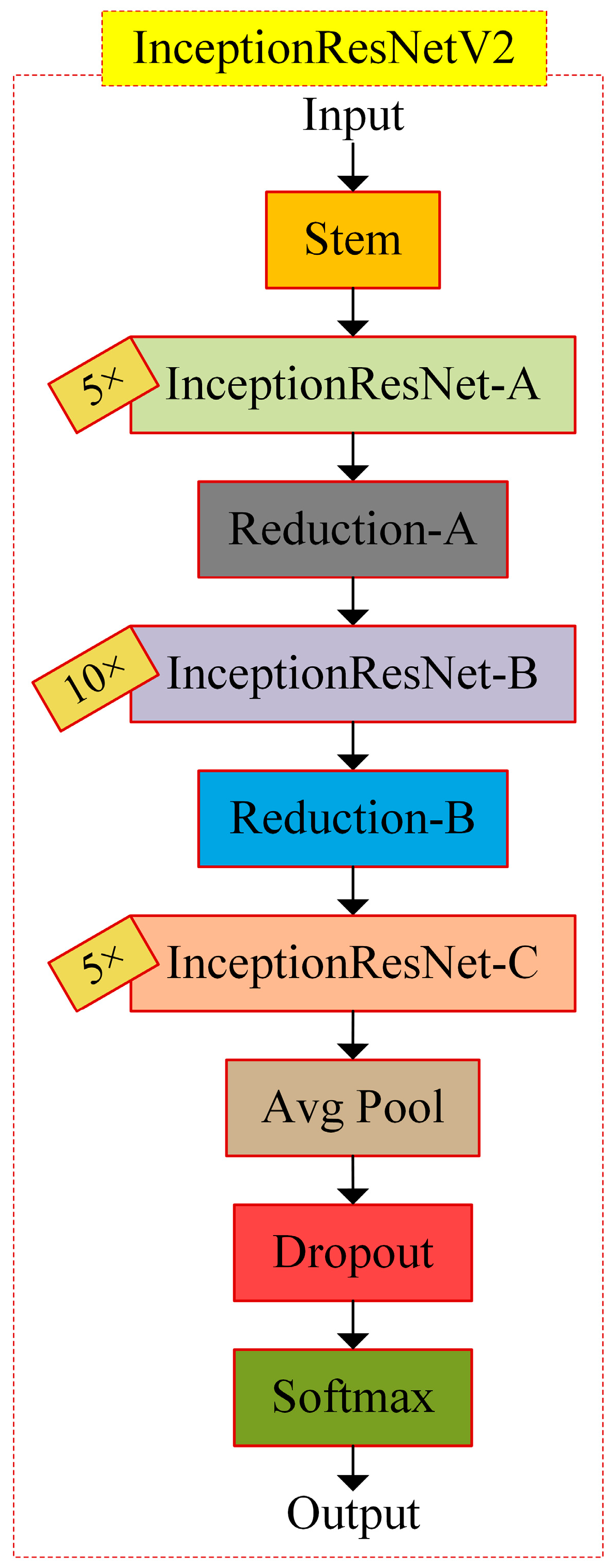
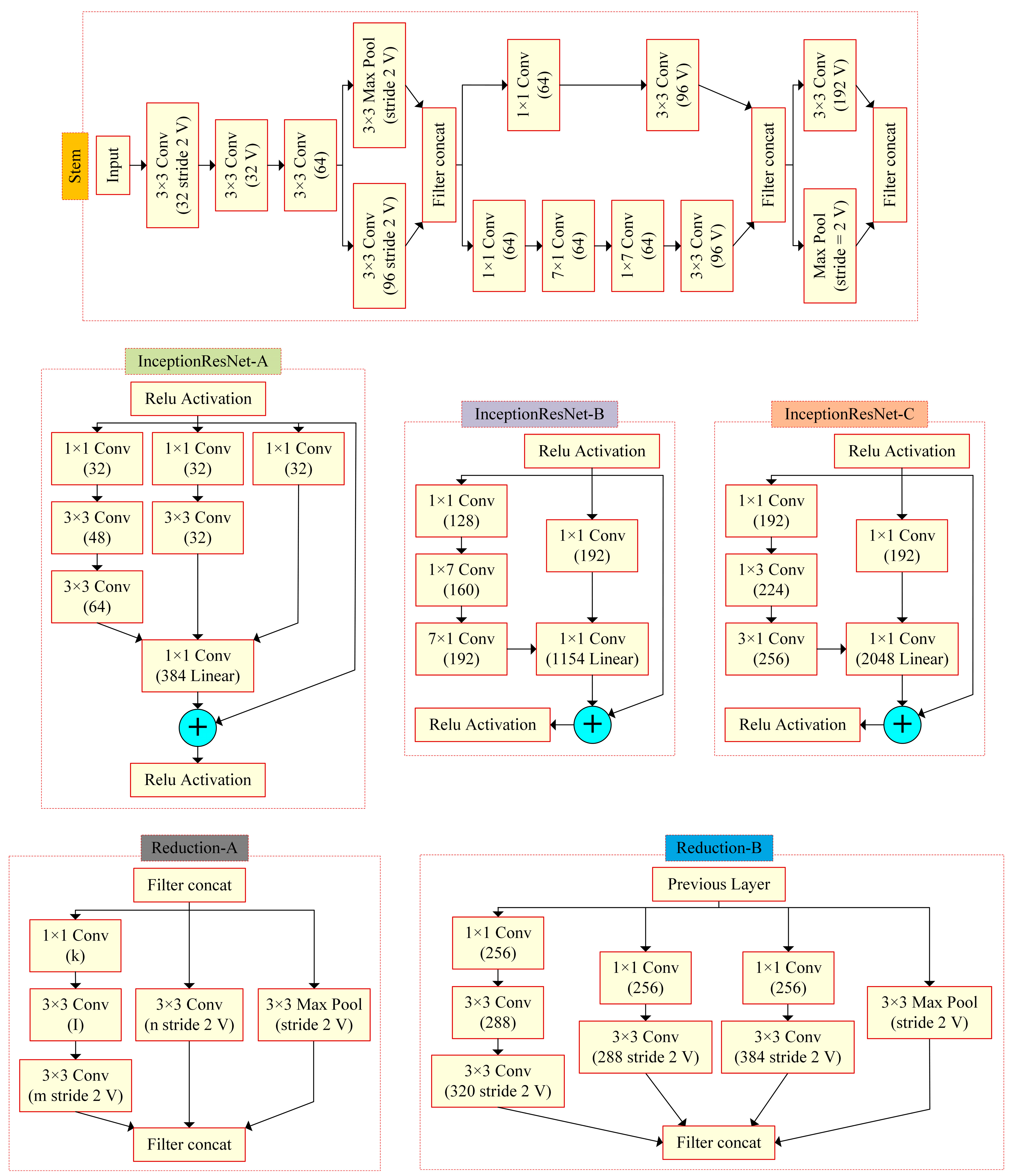
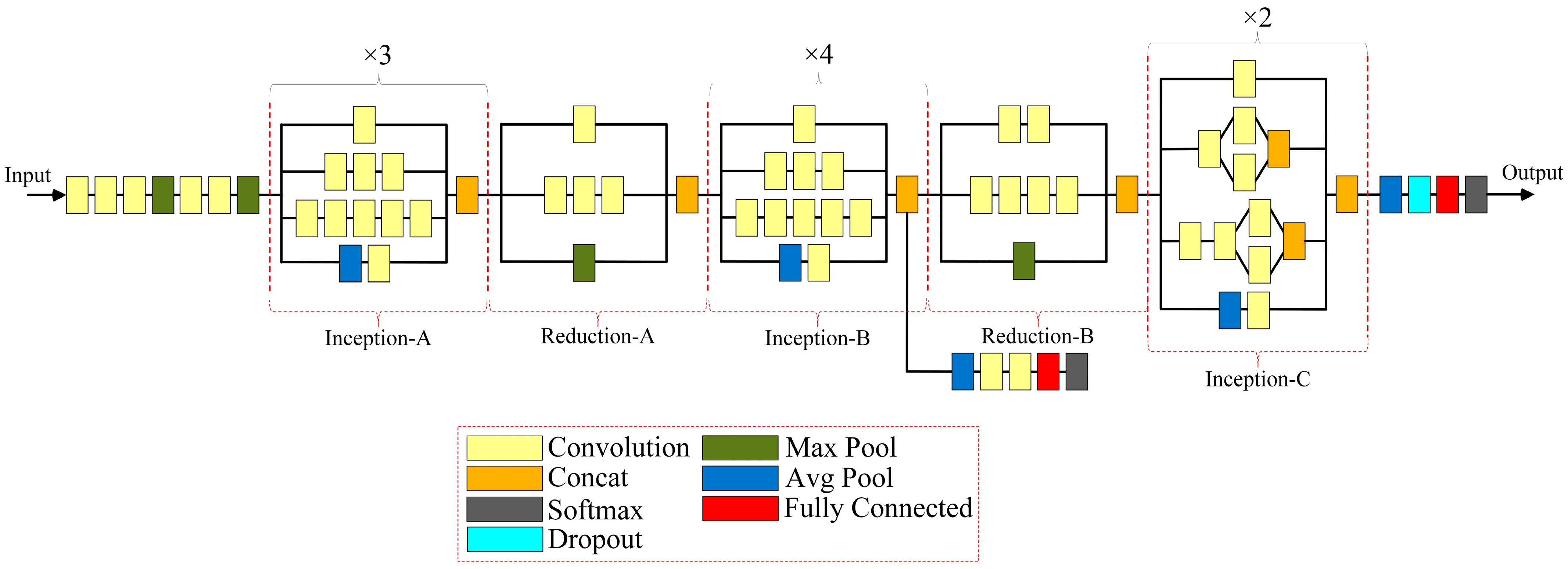
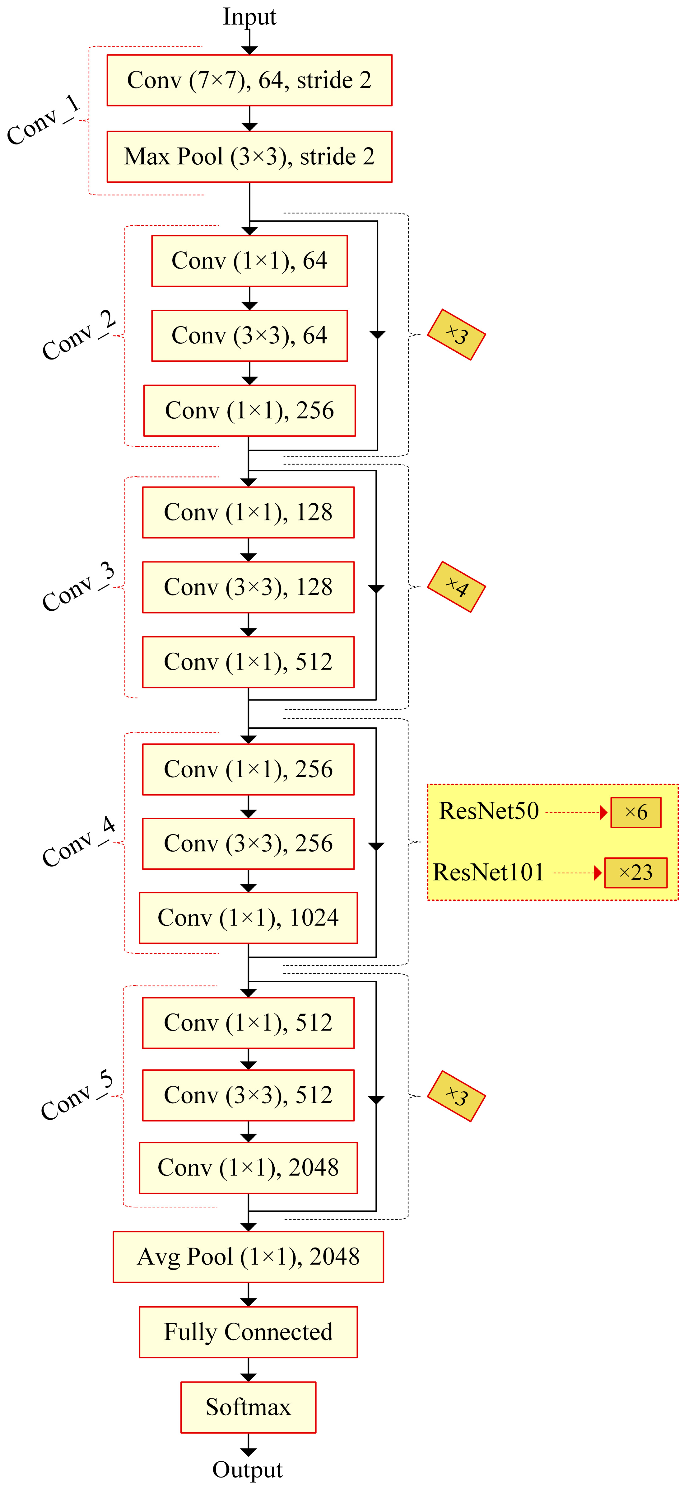
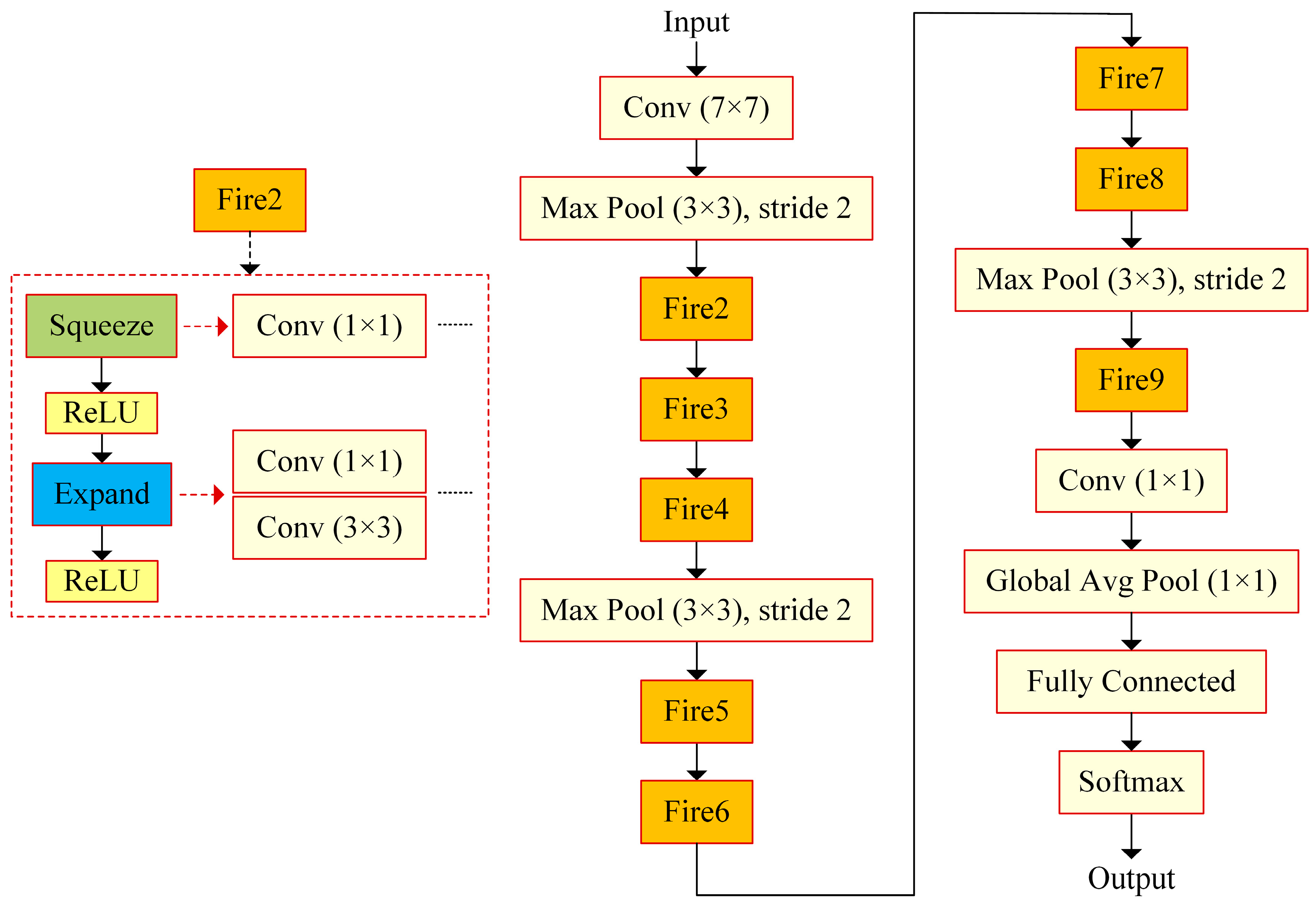
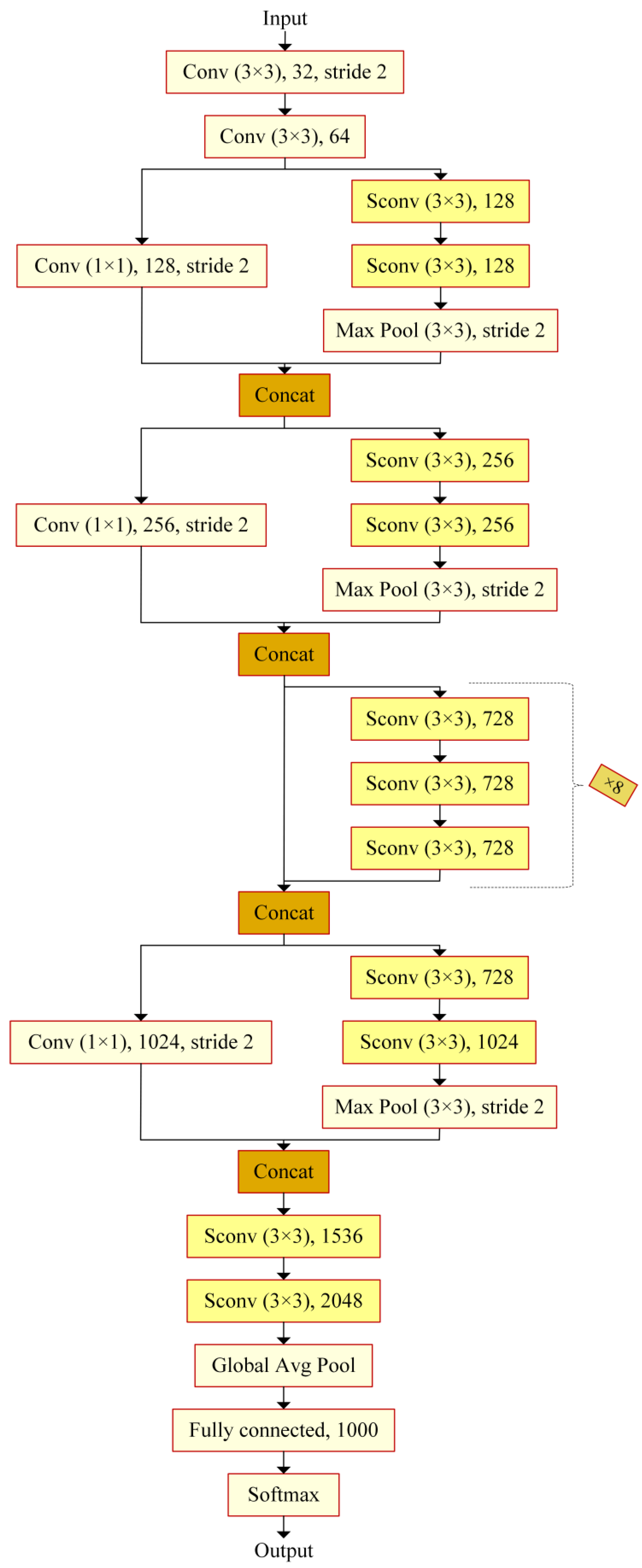
In this paper, eight transfer learning architectures, DenseNet201, InceptionResNetV2, InceptionV3, ResNet50, ResNet101, SqueezeNet, VGG19, and Xception, are examined in detail with their hyperparameters and are compared with each other to detect the most appropriate one with the data utilized. The data obtained as the result of the 3t2FTS approach were directly fed to the input of deep learning models. In this way, a novel framework handling HGG/LGG classification is presented. The experiments were performed using a two-fold cross-validation test method so as to evaluate the models in a comprehensive manner. All analyses were performed in the Deep Network Designer toolbox of MATLAB software on a personal computer with a 2.60 GHz CPU, 8 GB RAM, and Intel(R) Core(TM) i5-7200U graphic card.
Table 1 shows the hyperparameter evaluations of the utilized models. In Table 1, only significant parameters are considered to prevent the information loss of models that are already pre-trained with effective datasets. Regarding this, four parameters are alternated to achieve the highest performance of transfer learning architectures on the classification of HGG/LGG tumors.
Table 2, Table 3, Table 4, Table 5, Table 6, Table 7, Table 8 and Table 9 show the model results concerning the adjustments of hyperparameters for DenseNet201, InceptionResNetV2, InceptionV3, ResNet50, ResNet101, SqueezeNet, VGG19, and Xception respectively.
According to the results in Table 2, the average accuracy of sgdm in 24 trials (75.61%) is better in comparison with the scores of the adam (74.94%) and rmsprop (72.67%) optimizers. The LRDF of ‘0.2’ seems reliable and outperforms other preferences by achieving a 75.53% average accuracy among 18 trials. Furthermore, the learning rate of ‘0.0001’ arises as being more appropriate to use by obtaining a 75.24% average accuracy among 24 trials. The mini-batch size of ‘32’ overcomes the choice of ‘16’ by achieving a 1.45% better average accuracy and by obtaining a 75.20% average accuracy among 36 trials. By means of the average accuracy-based trials, DenseNet201 presents a 74.47% success score in 72 trials. In terms of the highest accuracy observed (79.30%), DenseNet201 operates the sgdm optimizer, an LRDF of ‘0.8’, a learning rate of ‘0.001’, and a mini-batch size of ‘32’.
In experiments of Table 3, it can be seen that the average accuracy of sgdm in 24 trials (75.37%) is higher in comparison with the scores of the adam (72.38%) and rmsprop (72.09%) optimizers. The LRDF of ‘0.4’ seems reliable and outperforms other preferences by achieving 73.65% average accuracy among 18 trials. Furthermore, the learning rate of ‘0.0001’ arises as being more appropriate to utilize by obtaining a 74.39% average accuracy among 24 trials. The mini-batch size of ‘32’ overcomes the choice of ‘16’ by achieving a 0.04% better average accuracy and by obtaining a 73.30% average accuracy among 36 trials. By means of the average-accuracy-based trials, InceptionResNetV2 presents a 73.28% success score in 72 trials. In terms of the highest accuracy observed (77.90%), InceptionResNetV2 generally operates the sgdm optimizer, an LRDF of ‘0.8, 0.6, 0.4, or 0.2’, a learning rate of ‘0.0001’, and a mini-batch size of ‘16’.
Concerning the trials in Table 4, it was revealed that the average accuracy of sgdm in 24 trials (75.16%) is better in comparison with the scores of the adam (72.65%) and rmsprop (71.64%) optimizers. The LRDF of ‘0.2’ seems reliable and outperforms other preferences by achieving 74.11% average accuracy among 18 trials. Furthermore, the learning rate of ‘0.001’ arises as being more appropriate to use by obtaining a 73.96% average accuracy among 24 trials. The mini-batch size of ‘32’ overcomes the choice of ‘16’ by achieving a 0.08% better average accuracy and by obtaining a 73.19% average accuracy among 36 trials. By means of the average accuracy-based trials, InceptionV3 presents a 73.15% success score in 72 trials. In terms of the highest accuracy observed (78.60%), InceptionV3 operates the sgdm optimizer, an LRDF of ‘0.6’, a learning rate of ‘0.001’, and a mini-batch size of ‘32’.
Regarding the trials in Table 5, the average accuracy of sgdm in 24 trials (74.88%) is higher in comparison with the scores of the adam (74.02%) and rmsprop (71.52%) optimizers. The LRDF of ‘0.4’ seems reliable and outperforms other preferences by achieving 74.68% average accuracy among 18 trials. Furthermore, the learning rate of ‘0.0001’ arises as being more appropriate to utilize by obtaining a 75.64% average accuracy among 24 trials. The mini-batch size of ‘32’ overcomes the choice of ‘16’ by achieving 0.09% better average accuracy and by obtaining a 73.52% average accuracy among 36 trials. By means of the average accuracy-based trials, ResNet50 presents a 73.47% success score in 72 trials. In terms of the highest accuracy observed (80%), ResNet50 operates the sgdm optimizer, an LRDF of ‘0.8 or 0.4’, a learning rate of ‘0.0001’, and a mini-batch size of ‘32’.
According to the results in Table 6, the average accuracy of sgdm in 24 trials (75.39%) is better in comparison with the scores of the adam (73.46%) and rmsprop (71.34%) optimizers. The LRDF of ‘0.4’ seems reliable and outperforms other preferences by achieving 73.87% average accuracy among 18 trials. Furthermore, the learning rate of ‘0.0001’ arises as being more appropriate to use by obtaining a 74.39% average accuracy among 24 trials. The mini-batch size of ‘16’ overcomes the choice of ‘32’ by achieving a 0.31% better average accuracy and by obtaining a 73.52% average accuracy among 36 trials. By means of the average accuracy-based trials, ResNet101 presents a 73.37% success score in 72 trials. In terms of the highest accuracy observed (77.89%), ResNet101 operates a learning rate of ‘0.0001’, a mini-batch size of ‘32’, sgdm optimizer and a LRDF of ‘0.4’ or an rmsprop optimizer and an LRDF of ‘0.6’.
In experiments of Table 7, it can be seen that the average accuracy of sgdm in 24 trials (73.94%) is higher in comparison with the scores of the adam (70.99%) and rmsprop (72.03%) optimizers. The LRDF of ‘0.6’ seems reliable and outperforms other preferences by achieving 73.78% average accuracy among 18 trials. Furthermore, the learning rate of ‘0.001’ arises as being more appropriate to utilize by obtaining a 73.90% average accuracy among 24 trials. The mini-batch size of ‘16’ overcomes the choice of ‘32’ by achieving a 1.59% better average accuracy and by obtaining a 73.12% average accuracy among 36 trials. By means of the average-accuracy-based trials, SqueezeNet presents a 72.32% success score in 72 trials. In terms of the highest accuracy observed (75.44%), SqueezeNet operates the sgdm optimizer, an LRDF of ‘0.2’, a learning rate of ‘0.001’, a mini-batch size of ‘16’ or an sgdm optimizer, an LRDF of ‘0.8’, a learning rate of ‘0.001’, a mini-batch size of ‘32’ or an adam optimizer, an LRDF of 0.4’, a learning rate of ‘0.0001’, a mini-batch size of ‘32’.
Concerning the trials in Table 8, it can be seen that the average accuracy of sgdm in 24 trials (74.85%) is better in comparison with the scores of the adam (73.67%) and rmsprop (72.62%) optimizers. The LRDF of ‘0.2’ seems reliable and outperforms other preferences by achieving 73.88% average accuracy among 18 trials. Furthermore, the learning rate of ‘0.0001’ arises as being more appropriate to use by obtaining a 74.21% average accuracy among 24 trials. The mini-batch size of ‘32’ overcomes the choice of ‘16’ by achieving a 0.08% better average accuracy and by obtaining a 73.75% average accuracy among 36 trials. By means of the average-accuracy-based trials, VGG19 presents a 73.71% success score in 72 trials. In terms of the highest accuracy observed (78.25%), VGG19 operates the sgdm optimizer, an LRDF of ‘0.2’, a learning rate of ‘0.0001’, and a mini-batch size of ‘32’.
Regarding the trials in Table 9, the average accuracy of adam in 24 trials (73.95%) is higher in comparison with the scores of the sgdm (73.45%) and rmsprop (71.20%) optimizers. The LRDF of ‘0.2’ seems reliable and outperforms other preferences by achieving 73.68% average accuracy among 18 trials. Furthermore, the learning rate of ‘0.001’ arises as being more appropriate to utilize by obtaining a 73.35% average accuracy among 24 trials. The mini-batch size of ‘16’ overcomes the choice of ‘32’ by achieving a 1.61% better average accuracy and by obtaining a 73.67% average accuracy among 36 trials. By means of the average-accuracy-based trials, Xception presents a 72.87% success score in 72 trials. In terms of the highest accuracy observed (76.49%), Xception operates the sgdm optimizer, a mini-batch size of ‘16’, an LRDF of ‘0.2’, and a learning rate of ‘0.01’ or the sgdm optimizer, an LRDF of ‘0.4’, a learning rate of ‘0.001’, and a mini-batch size of ‘16’ or the rmsprop optimizer, an LRDF of ‘0.8’, a learning rate of ‘0.0001’, and a mini-batch size of ‘16’.

4. Discussion

As seen in the evaluations of Section 3, it can be seen that all deep learning models obtain very close results that reveal the necessity of an in-depth analysis of the observed scores. Among experiments, a two-fold cross-validation is operated as the test method, and other test methods (50%-50% or 70%-30% training-test split, etc.) are not considered. Concerning the literature studies that utilize deep learning methods, data augmentation is often preferred which cannot be handled in our research. In other words, our aim is to enforce the frameworks operating 3t2FTS and a transfer learning model without data augmentation but with sufficient training data. In addition, 2D-ID input images are not appropriate to apply data augmentation.
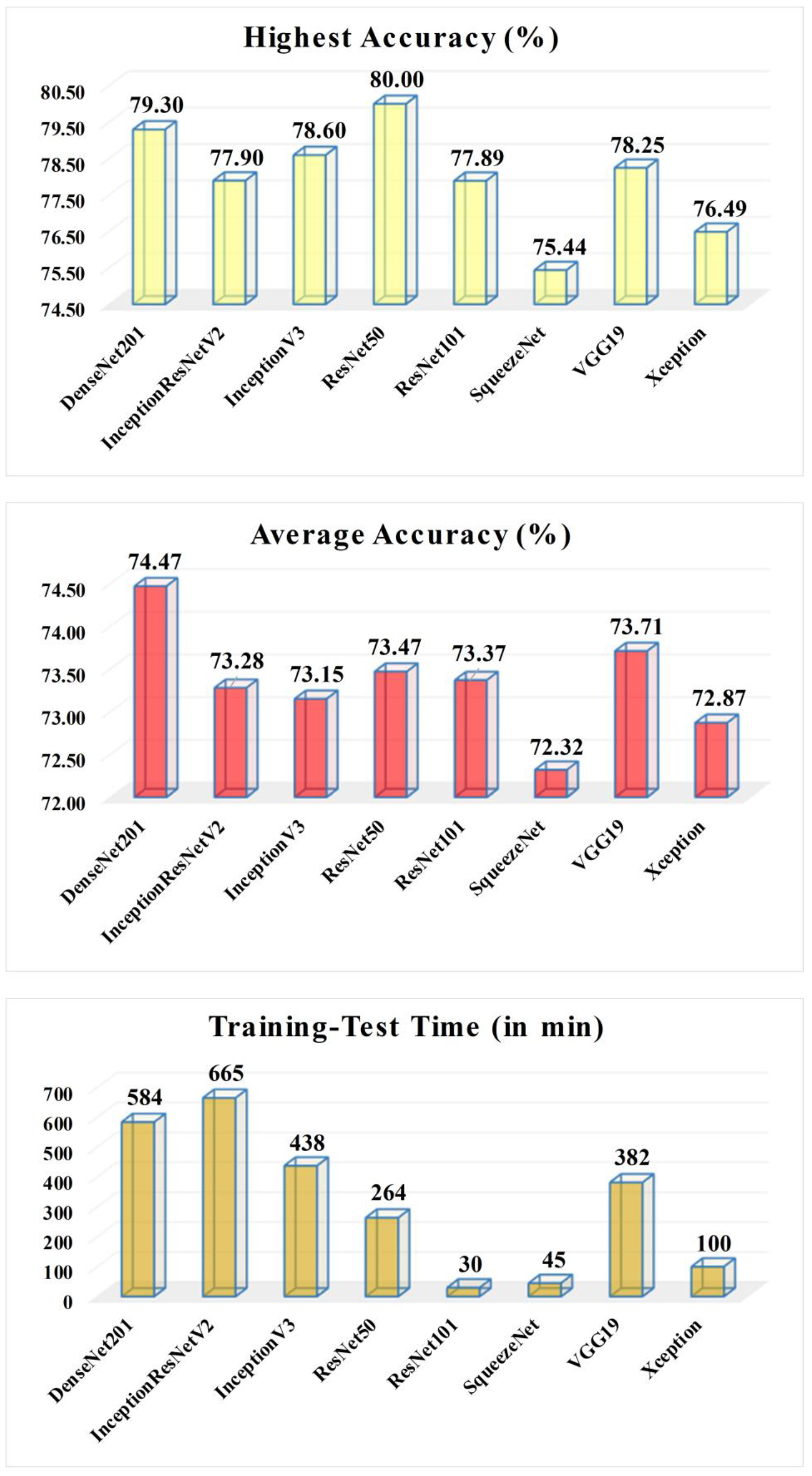
To reveal an in-depth analysis of the frameworks involving 3t2FTS and deep learning models, Figure 11 shows the comparison of transfer learning architectures by means of the highest accuracy-, average accuracy-, and computation-time-based evaluations.
Regarding the results in Section 3 and in Figure 11, it was revealed that:
  • The transfer learning models generally tend to produce higher performance by operating lower learning rates and the sgdm optimizer. Regarding the LRDF rate and mini-batch size, there is no distinct assignment to be defined and these parameters can change from one model to another.
  • The highest accuracy is achieved by the ResNet50 model, whilst DenseNet201 and InceptionV3 obtain the second- and third-best accuracies, respectively.
  • The highest average accuracy is recorded by DenseNet201 architecture, while in the meantime, VGG19 and ResNet50 acquire the second- and third-best scores, respectively. In other words, these models are seen as the most robust architectures among others.
  • The least computation time is attained by ResNet101, while the SqueezeNet and Xception models have the second- and third-best operation times, respectively. In addition, ResNet50 comes to the forefront by resulting in 264min and by having the fourth-best performance.
  • Concerning the aforementioned discussions and deductions, it was revealed that DenseNet201 comes as the second-best preference regarding the highest average accuracy and the second-best highest accuracy scores. However, its computation time is the second worst one which is about 584min for the training-test time.
  • As one of the three robust models, by achieving the highest classification accuracy and resulting in less time in particular than the DenseNet201, InceptionV3, and VGG19 models, ResNet50 comes forward due to the operation time- and accuracy-based in-depth evaluations.
The ResNet50 architecture arises as the most appropriate one to utilize with the 3t2FTS approach by recording the highest accuracy, a robust average performance, and less operation time in comparison with the robust models (DenseNet201 and VGG19) so as to perform the HGG vs. LGG categorization.
In the literature, there exists the study of Koyuncu et al. [14] directly classifying the HGG- vs. LGG-type tumors in 3D. In [14], there exists an efficient, statistical, and experimental framework, and a deep learning-based system is not available in the literature which proves and motivates the importance of our study.
In summary, our framework including 3t2FTS and ResNet50 achieves good performance, and this performance is open to being enhanced. In other words, 3t2FTS can be inferred as a novel strategy and different deep learning architectures can be applicable to the output of the 3t2FTS which will guide the literature on various research areas. In addition, a novel deep learning model can be produced to operate with only 3t2FTS output which will constitute another research area. Herein, concerning our results, ResNet50-based various frameworks can yield better performance too.

5. Conclusions

In this paper, a promising framework evaluating the classification of HGG- vs LGG-type tumors was performed using a novel feature extraction strategy named 3t2FTS and the ResNet50 transfer learning architecture. 3t2FTS can also be utilized to discriminate different kinds of tumors in 3D MRI images since it summarizes the 3D voxel by transforming the space from 3D to 2D. In addition, 3t2FTS arises as a space transform strategy using radiomics, unlike quantitative multi-parameter mapping which aims to transform the appearance of the stabilized brain tissue [37,38,39]. Moreover, 3t2FTS reveals a new phenomenon that is open to improvement by means of finding a coherent deep learning architecture. For our study, ResNet50 comes to the forefront among seven qualified transfer learning architectures on tumor grading as a result of accuracy- and computation-time-based in-depth evaluations. In addition, sgdm and low learning rates also attract notice as the most repeated optimizer and learning rate adjustments for deep learning models, respectively. Consequently, efficient research to be determined for guiding 3D MRI-based classification tasks is presented in the literature.
In future work, we want to generate a new deep learning framework that includes ResNet50 logic in the main part. Furthermore, various tumors scanned in 3D MRI can be handled to approve the efficiency of 3t2FTS and novel deep learning strategies. In addition, it can be a good idea to utilize an MRI dataset including some artifacts and distortions which can be examined to better applicate the framework or to directly design a robust framework.

Author Contributions

Conceptualization, H.K.; methodology, A.H. and H.K.; software, A.H. and H.K.; validation, A.H.; formal analysis, A.H.; investigation, A.H. and H.K.; resources, A.H.; data curation, A.H.; writing—original draft preparation, A.H. and H.K.; writing—review and editing, A.H. and H.K.; visualization, H.K.; supervision, H.K. All authors have read and agreed to the published version of the manuscript.

Funding

This research received no external funding.

Institutional Review Board Statement

Not applicable.

Informed Consent Statement

Not applicable.

Data Availability Statement

In this study, we used a publicly available MRI dataset: BraTS 2017/2018.

Acknowledgments

This work was supported by the Coordinatorship of Konya Technical University’s Scientific Research Projects.

Conflicts of Interest

The authors declare no conflict of interest. The funders had no role in the design of the study; in the collection, analysis, or interpretation of data; in the writing of the manuscript; or in the decision to publish the results.

References

  1. Latif, G.; Iskandar, D.A.; Alghazo, J.M.; Mohammad, N. Enhanced MR image classification using hybrid statistical and wavelets features. IEEE Access 2018, 7, 9634–9644. [Google Scholar] [CrossRef]
  2. Kumar, R.; Gupta, A.; Arora, H.S.; Pandian, G.N.; Raman, B. CGHF: A computational decision support system for glioma classification using hybrid radiomics-and stationary wavelet-based features. IEEE Access 2020, 8, 79440–79458. [Google Scholar] [CrossRef]
  3. Saba, T.; Mohamed, A.S.; El-Affendi, M.; Amin, J.; Sharif, M. Brain tumor detection using fusion of hand crafted and deep learning features. Cogn. Syst. Res. 2020, 59, 221–230. [Google Scholar] [CrossRef]
  4. Gupta, N.; Bhatele, P.; Khanna, P. Glioma detection on brain MRIs using texture and morphological features with ensemble learning. Biomed. Signal Proces. 2019, 47, 115–125. [Google Scholar] [CrossRef]
  5. Sharif, M.; Amin, J.; Nisar, M.W.; Anjum, M.A.; Muhammad, N.; Shad, S.A. A unified patch based method for brain tumor detection using features fusion. Cogn. Syst. Res. 2020, 59, 273–286. [Google Scholar] [CrossRef]
  6. Fang, L.; Wang, X.; Lian, Z.; Yao, Y.; Zhang, Y. Supervoxel-based brain tumor segmentation with multimodal MRI images. Signal Image Video Process. 2022, 16, 1215–1223. [Google Scholar] [CrossRef]
  7. Li, P.; Wu, W.; Liu, L.; Serry, F.M.; Wang, J.; Han, H. Automatic brain tumor segmentation from Multiparametric MRI based on cascaded 3D U-Net and 3D U-Net++. Biomed. Signal Proces. 2022, 78, 103979. [Google Scholar] [CrossRef]
  8. Kronberg, R.M.; Meskelevicius, D.; Sabel, M.; Kollmann, M.; Rubbert, C.; Fischer, I. Optimal acquisition sequence for AI-assisted brain tumor segmentation under the constraint of largest information gain per additional MRI sequence. Neurosci. Inf. 2022, 2, 100053. [Google Scholar] [CrossRef]
  9. Ghaffari, M.; Samarasinghe, G.; Jameson, M.; Aly, F.; Holloway, L.; Chlap, P.; Koh, E.-S.; Sowmya, A.; Oliver, R. Automated post-operative brain tumour segmentation: A deep learning model based on transfer learning from pre-operative images. Magn. Reson. Imaging 2022, 86, 28–36. [Google Scholar] [CrossRef] [PubMed]
  10. Wang, S.; Wang, H.; Shen, Y.; Wang, X. Automatic recognition of mild cognitive impairment and alzheimers disease using ensemble based 3D densely connected convolutional networks. In Proceedings of the 2018 17th IEEE International Conference on Machine Learning and Applications (ICMLA), Orlando, FL, USA, 17–20 December 2018; pp. 517–523. [Google Scholar]
  11. Wang, H.; Shen, Y.; Wang, S.; Xiao, T.; Deng, L.; Wang, X.; Zhao, X. Ensemble of 3D densely connected convolutional network for diagnosis of mild cognitive impairment and Alzheimer’s disease. Neurocomputing 2019, 333, 145–156. [Google Scholar] [CrossRef]
  12. Yu, W.; Lei, B.; Ng, M.K.; Cheung, A.C.; Shen, Y.; Wang, S. Tensorizing GAN with high-order pooling for Alzheimer’s disease assessment. IEEE Trans. Neur. Net. Lear. 2021, 33, 4945–4959. [Google Scholar] [CrossRef]
  13. Bodapati, J.D.; Shaik, N.S.; Naralasetti, V.; Mundukur, N.B. Joint training of two-channel deep neural network for brain tumor classification. Signal Image Video Process. 2021, 15, 753–760. [Google Scholar] [CrossRef]
  14. Koyuncu, H.; Barstuğan, M.; Öziç, M.Ü. A comprehensive study of brain tumour discrimination using phase combinations, feature rankings, and hybridised classifiers. Med. Biol. Eng. Comput. 2020, 58, 2971–2987. [Google Scholar] [CrossRef]
  15. Materka, A.; Strzelecki, M. Texture analysis methods—A review. COST B11 Rep. 1998, 10, 4968. [Google Scholar]
  16. Koyuncu, H.; Barstuğan, M. COVID-19 discrimination framework for X-ray images by considering radiomics, selective information, feature ranking, and a novel hybrid classifier. Signal Process. Image Commun. 2021, 97, 116359. [Google Scholar] [CrossRef]
  17. Sakalli, G.; Koyuncu, H. Discrimination of electrical motor faults in thermal images by using first-order statistics and classifiers. In Proceedings of the 2022 International Congress on Human-Computer Interaction, Optimization and Robotic Applications (HORA), Ankara, Türkiye, 9–11 June 2022; pp. 1–5. [Google Scholar]
  18. Menze, B.H.; Jakab, A.; Bauer, S.; Kalpathy-Cramer, J.; Farahani, K.; Kirby, J.; Burren, Y.; Porz, N.; Slotboom, J.; Wiest, R.; et al. The multimodal brain tumor image segmentation benchmark (BRATS). IEEE Trans. Med. Imaging 2014, 34, 1993–2024. [Google Scholar] [CrossRef]
  19. Bakas, S.; Akbari, H.; Sotiras, A.; Bilello, M.; Rozycki, M.; Kirby, J.S.; Freymann, J.B.; Farahani, K.; Davatzikos, C. Advancing the cancer genome atlas glioma MRI collections with expert segmentation labels and radiomic features. Sci. Dat. 2017, 4, 170117. [Google Scholar] [CrossRef] [PubMed] [Green Version]
  20. Bakas, S.; Reyes, M.; Jakab, A.; Bauer, S.; Rempfler, M.; Crimi, A.; Shinohara, R.T.; Berger, C.; Ha, S.M.; Rozycki, M.; et al. Identifying the best machine learning algorithms for brain tumor segmentation, progression assessment, and overall survival prediction in the BRATS challenge. arXiv 2018, arXiv:1811.02629. [Google Scholar]
  21. Huang, G.; Liu, Z.; Van Der Maaten, L.; Weinberger, K.Q. Densely connected convolutional networks. In Proceedings of the IEEE Conference on Computer Vision and Pattern Recognition (CVPR), Honolulu, HI, USA, 21–26 July 2017; pp. 4700–4708. [Google Scholar]
  22. Jaiswal, A.; Gianchandani, N.; Singh, D.; Kumar, V.; Kaur, M. Classification of the COVID-19 infected patients using DenseNet201 based deep transfer learning. J. Biomol. Struct. Dyn. 2021, 39, 5682–5689. [Google Scholar] [CrossRef] [PubMed]
  23. Szegedy, C.; Ioffe, S.; Vanhoucke, V.; Alemi, A.A. Inception-v4, inception-resnet and the impact of residual connections on learning. In Proceedings of the Thirty-First AAAI Conference on Artificial Intelligence (AAAI), San Francisco, CA, USA, 4–9 February 2017; pp. 4278–4284. [Google Scholar]
  24. Hassan, S.M.; Maji, A.K.; Jasiński, M.; Leonowicz, Z.; Jasińska, E. Identification of plant-leaf diseases using CNN and transfer-learning approach. Electronics 2021, 10, 1388. [Google Scholar] [CrossRef]
  25. Szegedy, C.; Vanhoucke, V.; Ioffe, S.; Shlens, J.; Wojna, Z. Rethinking the inception architecture for computer vision. In Proceedings of the IEEE Conference on Computer Vision and Pattern Recognition (CVPR), Las Vegas, NV, USA, 27–30 June 2016; pp. 2818–2826. [Google Scholar]
  26. Mahdianpari, M.; Salehi, B.; Rezaee, M.; Mohammadimanesh, F.; Zhang, Y. Very deep convolutional neural networks for complex land cover mapping using multispectral remote sensing imagery. Remote Sens. 2018, 10, 1119. [Google Scholar] [CrossRef] [Green Version]
  27. Al Husaini, M.A.S.; Habaebi, M.H.; Gunawan, T.S.; Islam, M.R.; Elsheikh, E.A.; Suliman, F.M. Thermal-based early breast cancer detection using inception V3, inception V4 and modified inception MV4. Neural. Comput. Appl. 2022, 34, 333–348. [Google Scholar] [CrossRef]
  28. Rao, A.S.; Nguyen, T.; Palaniswami, M.; Ngo, T. Vision-based automated crack detection using convolutional neural networks for condition assessment of infrastructure. Struct. Hlth. Monit. 2021, 20, 2124–2142. [Google Scholar] [CrossRef]
  29. He, K.; Zhang, X.; Ren, S.; Sun, J. Deep residual learning for image recognition. In Proceedings of the IEEE Conference on Computer Vision and Pattern Recognition (CVPR), Las Vegas, NV, USA, 27–30 June 2016; pp. 770–778. [Google Scholar]
  30. Kim, Y.H.; Park, J.B.; Chang, M.S.; Ryu, J.J.; Lim, W.H.; Jung, S.K. Influence of the depth of the convolutional neural networks on an artificial intelligence model for diagnosis of orthognathic surgery. J. Pers. Med. 2021, 11, 356. [Google Scholar] [CrossRef] [PubMed]
  31. Iandola, F.N.; Han, S.; Moskewicz, M.W.; Ashraf, K.; Dally, W.J.; Keutzer, K. SqueezeNet: AlexNet-level accuracy with 50× fewer parameters and <0.5 MB model size. arXiv 2016, arXiv:1602.07360. [Google Scholar]
  32. Li, Q.; Yang, Y.; Guo, Y.; Li, W.; Liu, Y.; Liu, H.; Kang, Y. Performance evaluation of deep learning classification network for image features. IEEE Access 2021, 9, 9318–9333. [Google Scholar] [CrossRef]
  33. Simonyan, K.; Zisserman, A. Very deep convolutional networks for large-scale image recognition. arXiv 2014, arXiv:1409.1556. [Google Scholar]
  34. Bansal, M.; Kumar, M.; Sachdeva, M.; Mittal, A. Transfer learning for image classification using VGG19: Caltech-101 image data set. J. Amb. Intel. Hum. Comp. 2021, 14, 3609–3620. [Google Scholar] [CrossRef]
  35. Chollet, F. Xception: Deep learning with depthwise separable convolutions. In Proceedings of the IEEE Conference on Computer Vision and Pattern Recognition (CVPR), Honolulu, HI, USA, 21–26 July 2017; pp. 1251–1258. [Google Scholar]
  36. Leonardo, M.M.; Carvalho, T.J.; Rezende, E.; Zucchi, R.; Faria, F.A. Deep feature-based classifiers for fruit fly identification (Diptera: Tephritidae). In Proceedings of the 31st SIBGRAPI Conference on Graphics, Patterns and Images (SIBGRAPI), Parana, Brazil, 29 October–1 November 2018; pp. 41–47. [Google Scholar]
  37. Cooper, G.; Hirsch, S.; Scheel, M.; Brandt, A.U.; Paul, F.; Finke, C.; Boehm-Sturm, P.; Hetzer, S. Quantitative multi-parameter mapping optimized for the clinical routine. Front. Neurosci. 2020, 14, 611194. [Google Scholar] [CrossRef]
  38. Qiu, S.; Chen, Y.; Ma, S.; Fan, Z.; Moser, F.G.; Maya, M.M.; Christodoulou, A.G.; Xie, Y.; Li, D. Multiparametric mapping in the brain from conventional contrast-weighted images using deep learning. Magn. Reson. Med. 2022, 87, 488–495. [Google Scholar] [CrossRef]
  39. Ma, L.; Wu, J.; Yang, Q.; Zhou, Z.; He, H.; Bao, J.; Wang, X.; Zhang, P.; Zhong, J.; Cai, C.; et al. Single-shot multi-parametric mapping based on multiple overlapping-echo detachment (MOLED) imaging. Neuroimage 2022, 263, 119645. [Google Scholar] [CrossRef] [PubMed]
Figure 1. Design steps of the 3D to 2D feature transform strategy.
Make 05 00022 g001
Figure 2. Handicaps of the dataset (1-3D view, 2-Cross sectional view).
Make 05 00022 g002
Figure 3. Architecture of the DenseNet201 model.
Make 05 00022 g003
Figure 4. Architecture of the InceptionResNetV2 model.
Make 05 00022 g004
Figure 5. Modules of the InceptionResNetV2.
Make 05 00022 g005
Figure 6. Schematic view of the InceptionV3 model.
Make 05 00022 g006
Figure 7. Architectures of the ResNet50 and ResNet101 models.
Make 05 00022 g007
Figure 8. Architecture of the SqueezeNet model.
Make 05 00022 g008
Figure 9. Architecture of the VGG19 model.
Make 05 00022 g009
Figure 10. Architecture of the Xception model.
Make 05 00022 g010
Figure 11. In-depth evaluations via the highest accuracy, average accuracy, and operation time.
Make 05 00022 g011
Table 1. Hyperparameter settings for transfer learning models.
ParameterValue/Range
Epoch100
Mini-batch size16, 32
Learning rate0.01, 0.001, 0.0001
Learning Rate Drop Factor (LRDF)0.2, 0.4, 0.6, 0.8
OptimizerAdam, Rmsprop, Sgdm
Table 2. Results of the DenseNet201 model.
Mini-Batch SizeLearning RateLRDFOptimizerAccuracyLearning RateLRDFOptimizerAccuracyLearning RateLRDFOptimizerAccuracy
160.010.2Adam76.490.0010.2Adam74.740.00010.2Adam75.40
Sgdm74.74Sgdm75.44Sgdm76.84
Rmsprop49.12Rmsprop77.90Rmsprop74.04
0.4Adam71.930.4Adam71.930.4Adam76.49
Sgdm65.26Sgdm78.95Sgdm74.74
Rmsprop69.47Rmsprop74.04Rmsprop75.44
0.6Adam76.490.6Adam76.140.6Adam71.58
Sgdm74.04Sgdm78.25Sgdm76.14
Rmsprop73.68Rmsprop73.68Rmsprop75.10
0.8Adam76.490.8Adam75.440.8Adam74.39
Sgdm74.74Sgdm76.84Sgdm76.49
Rmsprop49.12Rmsprop66.32Rmsprop74.39
320.010.2Adam78.250.0010.2Adam74.390.00010.2Adam75.09
Sgdm69.12Sgdm77.54Sgdm75.79
Rmsprop71.93Rmsprop75.09Rmsprop76.84
0.4Adam78.250.4Adam76.490.4Adam75.01
Sgdm77.54Sgdm74.74Sgdm75.09
Rmsprop71.93Rmsprop77.90Rmsprop76.84
0.6Adam71.230.6Adam70.180.6Adam73.68
Sgdm77.52Sgdm75.44Sgdm75.79
Rmsprop73.68Rmsprop65.61Rmsprop73.33
0.8Adam75.440.8Adam77.540.8Adam75.44
Sgdm76.84Sgdm79.30Sgdm75.79
Rmsprop74.39Rmsprop74.04Rmsprop76.14
Table 3. Results of the InceptionResNetV2 model.
Mini-Batch SizeLearning RateLRDFOptimizerAccuracyLearning RateLRDFOptimizerAccuracyLearning RateLRDFOptimizerAccuracy
160.010.2Adam74.040.0010.2Adam70.880.00010.2Adam73.68
Sgdm77.90Sgdm72.98Sgdm77.90
Rmsprop64.21Rmsprop73.33Rmsprop73.68
0.4Adam73.680.4Adam73.330.4Adam74.39
Sgdm75.09Sgdm76.84Sgdm77.90
Rmsprop73.68Rmsprop70.53Rmsprop73.68
0.6Adam72.280.6Adam74.740.6Adam74.39
Sgdm74.39Sgdm72.98Sgdm77.90
Rmsprop73.68Rmsprop68.42Rmsprop74.39
0.8Adam50.180.8Adam72.630.8Adam74.39
Sgdm76.49Sgdm72.63Sgdm77.90
Rmsprop73.33Rmsprop74.39Rmsprop74.39
320.010.2Adam70.880.0010.2Adam74.040.00010.2Adam71.58
Sgdm72.98Sgdm75.79Sgdm75.44
Rmsprop73.33Rmsprop75.09Rmsprop70.18
0.4Adam73.330.4Adam71.580.4Adam72.98
Sgdm76.84Sgdm72.98Sgdm76.14
Rmsprop70.53Rmsprop70.18Rmsprop71.93
0.6Adam74.740.6Adam73.680.6Adam74.74
Sgdm72.98Sgdm75.44Sgdm75.44
Rmsprop68.42Rmsprop71.93Rmsprop72.63
0.8Adam72.630.8Adam74.740.8Adam73.68
Sgdm72.63Sgdm75.79Sgdm75.44
Rmsprop74.39Rmsprop73.33Rmsprop70.53
Table 4. Results of the InceptionV3 model.
Mini-Batch SizeLearning RateLRDFOptimizerAccuracyLearning RateLRDFOptimizerAccuracyLearning RateLRDFOptimizerAccuracy
160.010.2Adam74.740.0010.2Adam75.090.00010.2Adam74.39
Sgdm75.80Sgdm76.84Sgdm73.68
Rmsprop73.68Rmsprop73.68Rmsprop73.68
0.4Adam74.740.4Adam72.280.4Adam74.74
Sgdm72.98Sgdm75.44Sgdm75.79
Rmsprop49.83Rmsprop73.68Rmsprop75.09
0.6Adam73.680.6Adam74.740.6Adam74.39
Sgdm77.19Sgdm77.19Sgdm76.84
Rmsprop56.14Rmsprop72.63Rmsprop73.68
0.8Adam72.980.8Adam70.530.8Adam74.74
Sgdm75.79Sgdm75.79Sgdm72.63
Rmsprop74.04Rmsprop72.98Rmsprop72.63
320.010.2Adam72.980.0010.2Adam72.980.00010.2Adam70.18
Sgdm70.18Sgdm75.44Sgdm78.25
Rmsprop73.68Rmsprop75.09Rmsprop73.68
0.4Adam73.680.4Adam73.680.4Adam68.07
Sgdm73.68Sgdm72.28Sgdm78.25
Rmsprop73.68Rmsprop76.49Rmsprop74.04
0.6Adam62.460.6Adam71.230.6Adam68.07
Sgdm73.33Sgdm78.60Sgdm76.49
Rmsprop72.98Rmsprop65.26Rmsprop72.98
0.8Adam75.090.8Adam75.090.8Adam72.98
Sgdm71.93Sgdm74.39Sgdm75.09
Rmsprop73.68Rmsprop73.68Rmsprop72.28
Table 5. Results of the ResNet50 model.
Mini-Batch SizeLearning RateLRDFOptimizerAccuracyLearning RateLRDFOptimizerAccuracyLearning RateLRDFOptimizerAccuracy
160.010.2Adam75.090.0010.2Adam71.220.00010.2Adam75.79
Sgdm74.74Sgdm74.74Sgdm76.84
Rmsprop73.68Rmsprop73.33Rmsprop74.04
0.4Adam74.040.4Adam76.140.4Adam75.09
Sgdm75.79Sgdm69.82Sgdm76.84
Rmsprop73.68Rmsprop73.68Rmsprop76.14
0.6Adam73.680.6Adam74.350.6Adam75.79
Sgdm74.39Sgdm74.73Sgdm76.84
Rmsprop68.07Rmsprop71.58Rmsprop74.04
0.8Adam75.440.8Adam71.930.8Adam75.09
Sgdm71.93Sgdm76.14Sgdm72.63
Rmsprop45.96Rmsprop75.79Rmsprop74.39
320.010.2Adam74.040.0010.2Adam71.580.00010.2Adam72.98
Sgdm75.44Sgdm71.23Sgdm78.60
Rmsprop73.33Rmsprop67.37Rmsprop74.74
0.4Adam75.790.4Adam73.680.4Adam75.79
Sgdm71.93Sgdm74.39Sgdm80.00
Rmsprop71.58Rmsprop74.39Rmsprop75.44
0.6Adam66.670.6Adam73.680.6Adam77.19
Sgdm72.63Sgdm76.49Sgdm73.68
Rmsprop70.53Rmsprop74.39Rmsprop72.28
0.8Adam74.040.8Adam71.580.8Adam75.79
Sgdm73.68Sgdm73.68Sgdm80.00
Rmsprop58.95Rmsprop73.68Rmsprop75.44
Table 6. Results of the ResNet101 model.
Mini-Batch SizeLearning RateLRDFOptimizerAccuracyLearning RateLRDFOptimizerAccuracyLearning RateLRDFOptimizerAccuracy
160.010.2Adam74.030.0010.2Adam69.820.00010.2Adam77.54
Sgdm76.14Sgdm76.14Sgdm76.49
Rmsprop73.68Rmsprop50.17Rmsprop75.38
0.4Adam73.680.4Adam77.190.4Adam75.08
Sgdm77.54Sgdm72.98Sgdm75.78
Rmsprop73.68Rmsprop68.72Rmsprop72.98
0.6Adam72.980.6Adam76.140.6Adam70.17
Sgdm75.78Sgdm73.33Sgdm73.68
Rmsprop73.68Rmsprop73.68Rmsprop70.87
0.8Adam75.080.8Adam72.280.8Adam75.08
Sgdm77.54Sgdm76.49Sgdm77.19
Rmsprop69.12Rmsprop73.68Rmsprop72.98
320.010.2Adam75.430.0010.2Adam74.430.00010.2Adam74.03
Sgdm74.43Sgdm76.49Sgdm75.38
Rmsprop67.01Rmsprop73.68Rmsprop77.19
0.4Adam75.430.4Adam68.720.4Adam70.17
Sgdm74.43Sgdm74.68Sgdm77.89
Rmsprop73.68Rmsprop74.68Rmsprop72.33
0.6Adam76.490.6Adam72.330.6Adam70.17
Sgdm74.38Sgdm76.14Sgdm76.84
Rmsprop65.96Rmsprop73.68Rmsprop77.89
0.8Adam72.980.8Adam74.430.8Adam69.47
Sgdm74.73Sgdm71.22Sgdm74.38
Rmsprop73.68Rmsprop57.19Rmsprop76.49
Table 7. Results of the SqueezeNet model.
Mini-Batch SizeLearning RateLRDFOptimizerAccuracyLearning RateLRDFOptimizerAccuracyLearning RateLRDFOptimizerAccuracy
160.010.2Adam73.680.0010.2Adam73.680.00010.2Adam71.23
Sgdm73.41Sgdm75.44Sgdm73.91
Rmsprop73.68Rmsprop73.68Rmsprop57.54
0.4Adam73.680.4Adam73.680.4Adam68.42
Sgdm74.41Sgdm73.91Sgdm73.68
Rmsprop73.68Rmsprop73.68Rmsprop72.98
0.6Adam73.680.6Adam73.680.6Adam72.98
Sgdm74.41Sgdm73.41Sgdm73.68
Rmsprop73.68Rmsprop73.68Rmsprop74.74
0.8Adam73.680.8Adam73.680.8Adam71.93
Sgdm73.68Sgdm75.08Sgdm73.68
Rmsprop73.68Rmsprop73.68Rmsprop74.74
320.010.2Adam49.830.0010.2Adam73.680.00010.2Adam72.98
Sgdm73.41Sgdm73.95Sgdm73.68
Rmsprop73.68Rmsprop73.68Rmsprop61.40
0.4Adam73.680.4Adam73.680.4Adam75.44
Sgdm73.68Sgdm73.91Sgdm73.68
Rmsprop73.68Rmsprop73.68Rmsprop74.04
0.6Adam73.680.6Adam73.680.6Adam73.68
Sgdm73.41Sgdm73.41Sgdm73.68
Rmsprop73.68Rmsprop73.68Rmsprop75.09
0.8Adam50.180.8Adam73.680.8Adam65.61
Sgdm73.95Sgdm75.44Sgdm73.68
Rmsprop73.68Rmsprop73.68Rmsprop59.30
Table 8. Results of the VGG19 model.
Mini-Batch SizeLearning RateLRDFOptimizerAccuracyLearning RateLRDFOptimizerAccuracyLearning RateLRDFOptimizerAccuracy
160.010.2Adam72.980.0010.2Adam71.230.00010.2Adam73.68
Sgdm75.44Sgdm75.09Sgdm73.33
Rmsprop70.88Rmsprop77.54Rmsprop72.63
0.4Adam73.680.4Adam75.090.4Adam71.23
Sgdm74.39Sgdm71.93Sgdm75.09
Rmsprop73.68Rmsprop75.09Rmsprop71.93
0.6Adam74.740.6Adam72.280.6Adam70.88
Sgdm76.49Sgdm77.90Sgdm77.54
Rmsprop72.28Rmsprop74.04Rmsprop73.68
0.8Adam75.090.8Adam76.840.8Adam74.39
Sgdm76.49Sgdm73.33Sgdm76.49
Rmsprop54.74Rmsprop77.54Rmsprop75.44
320.010.2Adam75.090.0010.2Adam73.680.00010.2Adam71.23
Sgdm74.04Sgdm75.79Sgdm78.25
Rmsprop70.53Rmsprop74.04Rmsprop74.39
0.4Adam75.790.4Adam70.880.4Adam75.44
Sgdm75.79Sgdm70.53Sgdm76.14
Rmsprop73.68Rmsprop75.44Rmsprop72.98
0.6Adam73.680.6Adam71.580.6Adam76.14
Sgdm72.98Sgdm72.28Sgdm72.98
Rmsprop73.68Rmsprop64.21Rmsprop75.44
0.8Adam74.740.8Adam73.680.8Adam74.04
Sgdm75.09Sgdm73.69Sgdm75.44
Rmsprop74.04Rmsprop72.63Rmsprop72.28
Table 9. Results of the Xception model.
Mini-Batch SizeLearning RateLRDFOptimizerAccuracyLearning RateLRDFOptimizerAccuracyLearning RateLRDFOptimizerAccuracy
160.010.2Adam73.680.0010.2Adam74.390.00010.2Adam72.28
Sgdm76.49Sgdm71.93Sgdm71.23
Rmsprop73.68Rmsprop74.39Rmsprop75.44
0.4Adam75.090.4Adam75.790.4Adam72.63
Sgdm71.93Sgdm76.49Sgdm71.23
Rmsprop73.68Rmsprop68.07Rmsprop72.63
0.6Adam73.680.6Adam75.090.6Adam71.23
Sgdm74.04Sgdm75.44Sgdm70.18
Rmsprop73.68Rmsprop72.98Rmsprop72.63
0.8Adam75.440.8Adam76.140.8Adam74.39
Sgdm71.93Sgdm73.68Sgdm74.74
Rmsprop73.68Rmsprop75.79Rmsprop76.49
320.010.2Adam74.740.0010.2Adam75.790.00010.2Adam72.63
Sgdm76.14Sgdm73.68Sgdm72.63
Rmsprop70.53Rmsprop74.74Rmsprop71.93
0.4Adam74.040.4Adam72.980.4Adam73.68
Sgdm72.63Sgdm72.98Sgdm75.44
Rmsprop71.23Rmsprop75.09Rmsprop73.68
0.6Adam74.040.6Adam74.390.6Adam71.93
Sgdm73.33Sgdm74.74Sgdm70.53
Rmsprop62.11Rmsprop57.90Rmsprop70.18
0.8Adam75.790.8Adam72.280.8Adam72.63
Sgdm75.44Sgdm70.88Sgdm75.09
Rmsprop53.33Rmsprop74.74Rmsprop70.18
Disclaimer/Publisher’s Note: The statements, opinions and data contained in all publications are solely those of the individual author(s) and contributor(s) and not of MDPI and/or the editor(s). MDPI and/or the editor(s) disclaim responsibility for any injury to people or property resulting from any ideas, methods, instructions or products referred to in the content.

