Alzheimer’s Disease Detection from Fused PET and MRI Modalities Using an Ensemble Classifier

Abstract

Alzheimer’s disease (AD) is an old-age disease that comes in different stages and directly affects the different regions of the brain. The research into the detection of AD and its stages has new advancements in terms of single-modality and multimodality approaches. However, sustainable techniques for the detection of AD and its stages still require a greater extent of research. In this study, a multimodal image-fusion method is initially proposed for the fusion of two different modalities, i.e., PET (Positron Emission Tomography) and MRI (Magnetic Resonance Imaging). Further, the features obtained from fused and non-fused biomarkers are passed to the ensemble classifier with a Random Forest-based feature selection strategy. Three classes of Alzheimer’s disease are used in this work, namely AD, MCI (Mild Cognitive Impairment) and CN (Cognitive Normal). In the resulting analysis, the Binary classifications, i.e., AD vs. CN and MCI vs. CN, attained an accuracy (A_cc) of 99% in both cases. The class AD vs. MCI detection achieved an adequate accuracy (A_cc) of 91%. Furthermore, the Multi Class classification, i.e., AD vs. MCI vs. CN, achieved 96% (A_cc).

1. Introduction

Alzheimer’s disease (AD) is a debilitating neurological disorder affecting millions worldwide. AD is now a leading cause of death in old age [1], and through trends, the number of cases will rise in the coming years. The biological reason for this condition is the build-up of a protein called beta-amyloid in the brain, leading to the loss of nerve cells [2]. Around 55 million people are affected by the severe neurological disorder known as dementia, with more than 60% of cases occurring in middle- and low-income countries. Economic, social, and mental stress are among the leading factors contributing to the onset of AD. As a result, there is a growing need to better understand the disease and identify effective treatments. In the modern era, using artificial intelligence (AI) techniques for detecting AD and its sub-stages is common practice [3]. These techniques include both single-modality and multimodality methods. However, though contributions from researchers have been made in this field, the most appropriate and effective methods have yet to be identified. AD has various biological and other causes, and the primary reasons cannot be placed through a single-modality approach [4]. In addition, there are other methods, such as clinical assessments, demographic conditions, and MMSE scores, but none have proven to be a sustainable approach for AD detection [5]. In their searching for a reliable method of detecting AD, many experts are exploring the use of a multimodal approach. This technique combines various biomarkers, such as MRI scans and PET scans, to diagnose more accurately [6].

In medical image fusion, combining different input images into a single fused image is a more natural method that provides essential and complementary information for accurate diagnosis and treatment. Pixel-level intensity matching is generally used in image fusion [7]. This approach, also known as multimodal fusion, is considered more efficient than feature fusion techniques as it expresses information more effectively and presents a broader range of features [8,9]. By fusing the components from different brain regions, a more precise visualization is possible, which can help identify the various stages of the disease, i.e., AD, Mild Cognitive Impairment (MCI), and Cognitive Normal (CN). This study compares Binary and Multi Class analysis for understanding the differences in AD. For classification, trending machine learning (ML) and ensemble learning (EL) techniques are utilized. Using a multi-model, multi-slice 2D CNN ensemble learning architecture is considered a highly effective approach for classifying AD versus CN and AD versus MCI, with an (A_cc) rate of 90.36% and 77.19%, respectively [10]. Another ensemble technique using the same architecture yielded (A_cc) rates of 90.36%, 77.19%, and 72.36% for AD, MCI, and CN, respectively, when compared to each other [11]. A new subset of three relevant features was used to create an ensemble model, and a weighted average of the top two classifiers (LR and linear SVM) was used. The voting classifier weighted average outperformed the basic classifiers, with an (A_cc) rate of 0.9799 ± 0.055 and an AUPR of 0.9108 ± 0.015 [12]. The CNN-EL ensemble classifier, using an MRI modality of the MCInc, yielded (A_cc) rates of 0.84 ± 0.05, 0.79 ± 0.04, and 0.62 ± 0.06 for identifying subjects with MCI or AD [13]. Bidirectional GAN is a revolutionary end-to-end network that uses image contexts and latent vectors to synthesize brain MR-to-PET images [14].

MRIs are generally used for the detection of AD. They are highly effective imaging tools and contain data related to the anatomy of the different neuro regions [15]. They reveal changes in brain structure before clinical symptoms appear. These modalities reflect alterations in the cortex, white matter (WM), and subcortical regions, which can help detect abnormalities caused by AD [16]. Brain shrinkage, which is frequent in AD, as well as the reduction in the size of specific brain areas such as the hippocampus (Hp), entorhinal cortex (Ec), temporal lobe (Tl), parietal lobe (Pl), and prefrontal cortex (Pc), have been observed [17]. These areas are critical for cognitive skills such as memory, perception, and speaking in AD [18]. The degree and pattern of atrophy in these areas can provide important visualizations for studying the prognosis of AD. MRI scans can detect lesions or anomalies in the brain that signal AD, for the early identification and therapy of the condition [19]. PET scans are generally for the diagnosis of AD [20]. PETs provide functional brain imaging by measuring glucose metabolism and detecting AD-associated brain function changes [21]. PET scans can detect amyloid plaques and Tau proteins, which signify AD, and measure glucose metabolism in the brain. Various PET modalities, such as amyloid PET, FDG-PET, and Tau PET, possess unique characteristics for identifying AD biomarkers. Amyloid PET employs a radiotracer to bind amyloid plaques, FDG-PET measures glucose metabolism, and Tau PET utilizes a radiotracer to bind Tau proteins, visually representing their presence in the brain.

Structural MRI can reveal alterations in brain structure, while functional PET images can capture the metabolic characteristics of the brain, enhancing the ability to detect lesions. FDG PET characteristics distinctly exhibit quantitative hypometabolism and a component in the precuneus among MCI patients. A volume-of-interest analysis comparing global GM in AD patients to healthy controls revealed reduced CBF and FDG uptake [22]. In a similar vein, MRI, FDG-PET, and CSF biomarkers were employed in a study to differentiate AD (or MCI) from healthy controls using a kernel combination strategy, with the combined method accurately identifying 91.5% of MCI converters and 73.4% of non-converters [23]. Both classifier-level and deep learning-based feature-level LUPI algorithms can enhance the performance of single-modal neuroimaging-based CAD for AD [24]. CERF integrates feature creation, feature selection, and sample classification to identify the optimal method combination and provide a framework for AD diagnosis [25]. Although these methods offer innovative frameworks, they still lack the ability to effectively detect AD and its subtypes. Consequently, it has been suggested that multimodal approaches combining MRI and PET images could improve the accuracy of AD classification. The fusion of PET and MRI images in machine learning has many advantages for analyzing and diagnosing neurological disorders such as AD [26]. Combining functional information from PET and structural details from MRI provides the models with a more extensive range of features, improving accuracy and strength. This integration compensates for individual modality limitations, allowing algorithms to utilize both imaging techniques’ strengths [27]. Machine learning models can better understand disease progression by capturing both functional and structural changes in the brain, ultimately improving early diagnosis, prognosis, and treatment planning. Hence, various performance metrics are compared for these classes to validate this study. The significant contribution made in this article is described here:

• This work proposes the image-fusion technique for the fusion of (PET + T1-weighted MRI) scans and feature fusion from the fused and non-fused imaging modalities for detecting AD.
• This work proposes the ensemble classification method (GB + SVM_RBF) for Multi Class classification and (SVM_RBF + ADA + GB + RF) methods for the Binary Class classification of AD.
• This work also reaches adequate (A_cc) in the Multi Class and the Binary Class classification of AD and its subtypes, i.e., (AD to MCI), which is 91%, and other classes (AD to CN) and (MCI to CN), with 99%. The (A_cc) achieved (AD vs. MCI vs. CN) in the Multi Class is 96%.

In this article, Section 2 delves into the previous research on AD detection and the importance of different methods in both single- and multimodal contexts, explicitly focusing on ML, DL, and EL methods. Section 3 provides detailed information about the data set used in the experiment, while Section 4 outlines the methodology, including various preprocessing techniques and the proposed image-fusion method. The results obtained from the ML and ensemble models (EL) are analyzed in Section 5, including Binary and Multi Class results, and the different trending methods used in the article are discussed. Lastly, Section 6 describes the conclusions of all the experimental works.

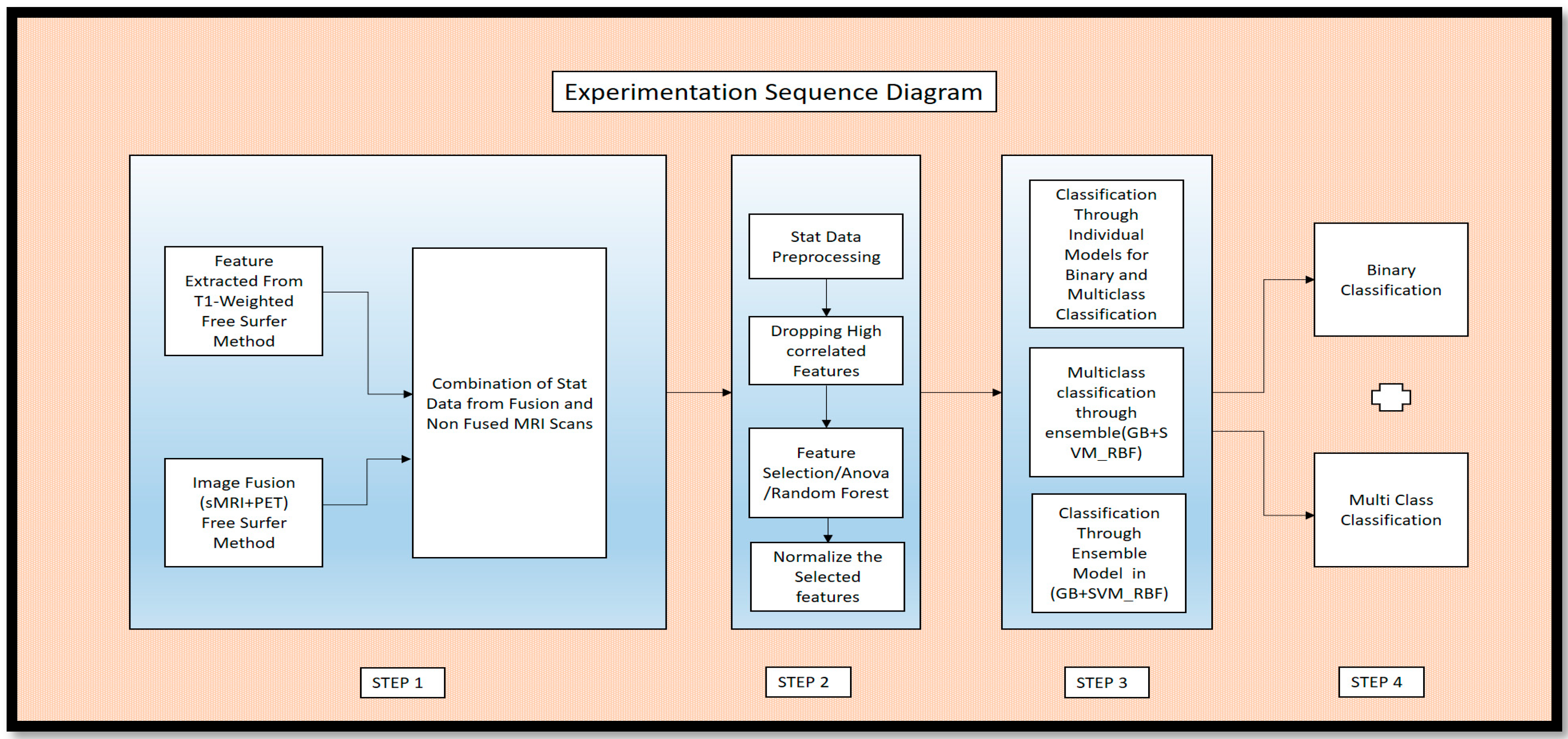
Figure 1 in the article provides an overview of the key experiments conducted in the study through an experimental sequence diagram. This figure outlines the basic experimental procedures described in the article.

2. Recent Study

Aged people are generally affected by AD; no prevention and cure diagnosis procedures are available for these patients. This disease is increasing drastically, and no decline has occurred [28]. Several studies have come into existence to tackle this issue, such as neuroimaging analysis to detect AD in the early stages [29]. AD detection can often be observed in one of the most common regions, namely the Hp region, by measuring its volume in affected patients. A decrease in the volume can result in the cause of AD [30]. To identify this reason, the semi-automatic segmentation technique ITK-SNAP concerns the age, gender, and left and right Hp volume values of AD patients [31]. Hence these values are taken as the neuroimaging data. These data, using factors such as age, visits, education, and MMSE, are processed using ML algorithms to predict AD [32]. The Extended Probabilistic Neural Network (EANN) and the Dynamic EL Algorithm (DELA) are also becoming trends in AD detection. The Logistic Regression (LR) method also has sustainable (A_cc) compared to the other methods.

Single modality and multimodality are ways of overriding the biomarkers. Neuroimaging also identifies the form of biomarkers to detect AD and its stages. Multimodality helps to identify the crucial hybrid set of features that can help diagnose and detect AD. These integrations are achieved through various ML and DL techniques [33]. DL methods also show some promising results in detecting AD and its stages, specifically MCI to AD conversion. They combine various data modalities to determine the difference between AD’s cortical and subcortical regions and their stages [34]. Multimodality in fluorescence optical imaging is used as biofuel for AD detection [35]. Fingerprints are common for the identification of AD. This approach also shows a more significant difference in the different stages of AD. Acoustic biomarkers play an essential role in the detection of subtypes of AD. These data types, when used and processed through the ML technique, provided 83.6% (A_cc) in AD and NC persons [36]. The retina attention is taken as a consideration for the identification of AD and other neuro disorders and diseases [37]. Cognitive scores, medication history, and demographic data also provide an effective source of information for classifying AD and subtypes using ML techniques [38]. Tri-modal approaches are also multimodal techniques for identifying hybrid features in the cortical region. Furthermore, ADx is an integrated diagnostic system that combines acoustics, microfluidics, and orthogonal biosensors for clinical purposes [39]. ML and adversarial hypergraph fusion are approaches for the prediction of AD and its stages [40].

A novel EL technique can accurately diagnose Alzheimer’s disease, even in its early stages. This approach enhances AD detection (A_cc) by integrating various classifiers from neuroimaging features and surpasses multiple state-of-the-art methods [41]. In this study, Alzheimer’s diagnostic precision was improved by applying the Decision Tree algorithm and three EL techniques to OASIS clinical data, with bagging achieving remarkable (A_cc) [42]. To attain a more accurate and reliable model, researchers propose an ensemble voting approach that combines multiple classifier predictions, yielding impressive results for older individuals in the OASIS data set [43]. This investigation introduces a unique computer-assisted method for early Alzheimer’s diagnosis, leveraging MRI images and various 3D classification architectures for image processing and analysis, further enhancing the EL technique’s outcomes [44].

For the detailed longitudinal studies of cortical regions of the brain, different state-of-the-art methods are available, including SVM, DT, RF, and KNN, which have shown the sustainable classification of the different stages of AD [45]. These come under the supervised learning approach and have been able to classify AD and its stages effectively [46]. A framework based on DL is used to identify individuals with various stages of AD, CN, and MCI [47]. In AD, the concatenation of MRI and PET scans using a wavelet transform-based multimodality fusion approach enables the prediction of AD [48]. To identify stages from MCI to AD, a multimodal RNN is used in the DL technique [49]. A comprehensive diagnostic tool detects AD and its stages using the hybrid cross-dimension neuroimaging biomarkers, longitudinal CSF, and cognitive score from the ADNI database [50]. A multimodal DL technique can also be used in clinical trials to identify individuals at high risk of developing AD [51].

These studies demonstrate the effectiveness of using DL and ML methods in single-, dual-, or tri-modality contexts for AD detection. One of the major challenges when employing DL methods for AD detection is the difficulty in visualizing or validating the precise features that contribute to AD identification and its stages. The DL approach makes it challenging to provide evidence for predicting and identifying the features responsible for AD. Moreover, DL methods require a large amount of labeled data for classifying AD and its stages. However, DL methods might necessitate even more data to accurately classify AD and its stages. To assist in AD diagnosis, an image-fusion technique known as ‘GM-PET’ combines MRI and FDG-PET grey matter (GM) brain tissue sections through registration and mask encoding. A 3D multi-scale CNN approach is utilized to assess its effectiveness [52]. In contrast, our research employs ensemble learning techniques to classify various subtypes. By incorporating ML methods, we perform in-depth analyses that enable us to pinpoint the precise AD-related regions within cortical and subcortical features while also evaluating the effectiveness of the fusion technique.

Therefore, ML methods offer several advantages over DL for detecting AD and its stages. They are often more straightforward to implement with detailed reasons about which causes AD and their subtypes. ML uses biomarker features like molecular, audio, fingerprints, structural MRI, functional MRI, PET scans, and clinical, which have shown good performance even with smaller data sets. ML models are preferred because they can better understand the factors that contribute to the disease and its stages. However, the challenges are still in the enormous amount of medical data. EL is favored over traditional ML models, as it can better comprehend the factors contributing to a disease and its progression. Despite the challenges of vast medical data sets and the quest for optimal (A_cc), EL techniques help overcome limitations. The diagnostic performance can be significantly improved compared to standard ML techniques. Even though DL has an advantage when dealing with complex data such as fMRI and PET, ML, and EL are practical approaches for detecting AD and its distinct stages.

3. Data Set

This data set has been taken from the Alzheimer Disease Neuroimaging Initiative (ADNI). All the images taken here are raw; they are not preprocessed. The database link is (adni.loni.usc.edu). Los Angeles, CA: Laboratory of Neuro Imaging, University of Southern California

Table 1. Data set used in this research.

S. No	Stages	Modality	Age	Gender	Quantity	Properties
1	AD	T1-weighted MRI	80–85	M/F	200	Raw and Non-Filtered
2	CN	T1-weighted MRI	82–85	M/F	200	Raw and Non-Filtered
3	MCI	T1-weighted MRI	74–87	M/F	200	Raw and Non-Filtered
4	AD	PET	85–86	M/F	200	Raw and Non-Filtered
5	CN	PET	70–84	M/F	200	Raw and Non-Filtered
6	MCI	PET	85–89	M/F	200	Raw and Non-Filtered

. The PET images were acquired in December, with the data set comprising various subjects from 2010 to 2022. The data were downloaded in November 2022 for preprocessing and feature extraction purposes, specifically for the PET modality of all AD, MCI, and CN subjects. In a similar vein, the sMRI data for AD, MCI, and CN subjects spanned from 2006 to 2014 and were downloaded in April 2022. Instead of subject-wise matching, only quantity and structural mapping were conducted for the analysis.

This table describes using two different modalities (T1-weighted MRI) and PET. These data sets are a combination of males and females. Their ages generally range between 70 and 90, and the average age is 80. A total number of 1200 images was used in this research work, and each stage, including AD, MCI, and CN, individually had 200 images. The quality of these images is raw and unfiltered and they were not processed anywhere. 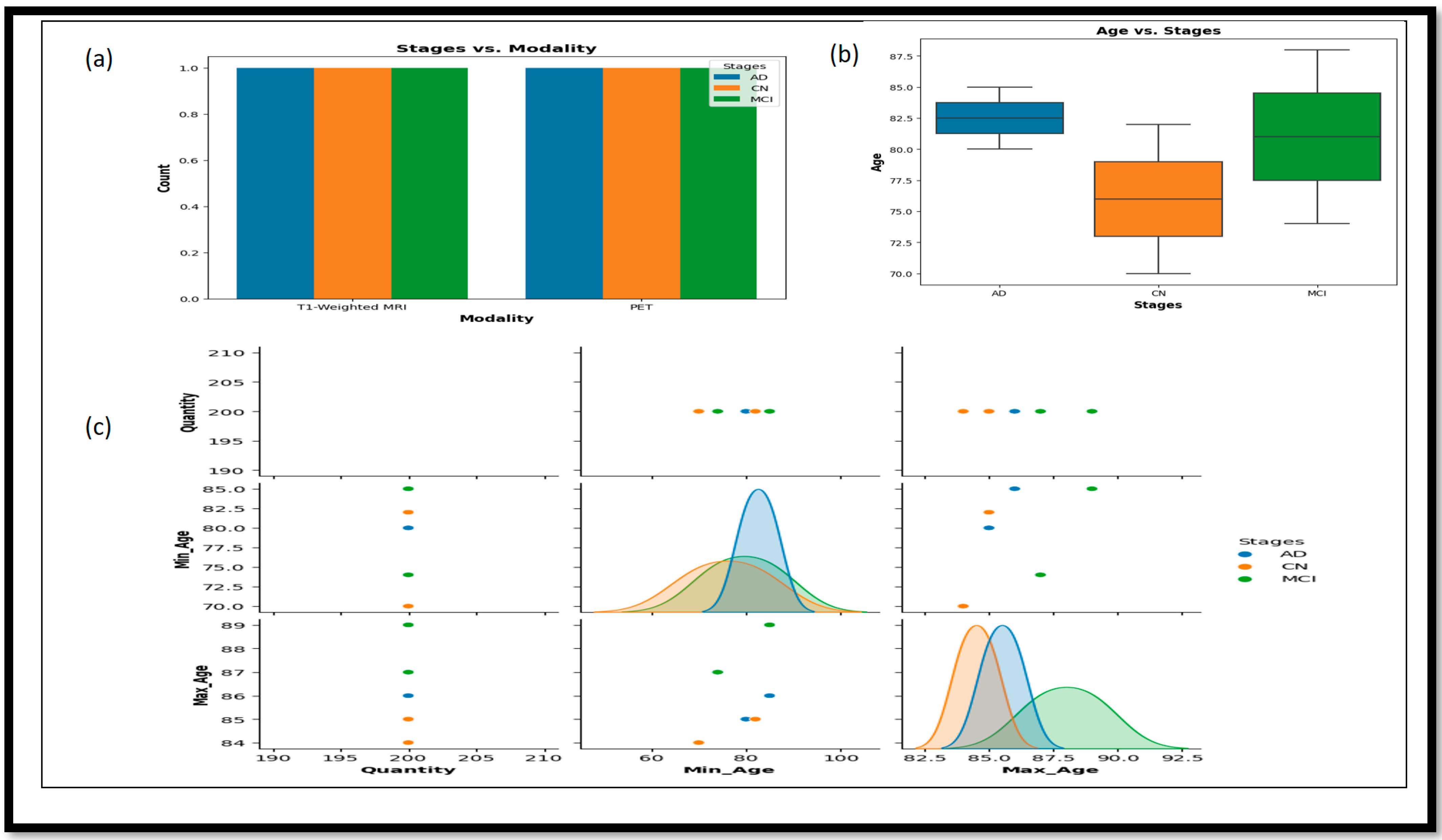Figure 2 provides more detailed information about the relationship between various attributes using different plots.

In Figure 2a, the bar plot represents the plot of Stages vs. Modality, which shows the distribution of different stages (AD, CN, and MCI) across the two imaging modalities—T1-weighted MRI and PET. Figure 2b, the box plot of Age vs. Stages, illustrates the age range distribution for each stage, highlighting the differences and similarities in age ranges among AD, CN, and MCI groups. Lastly, the Figure 2c pair plot showcases pairwise relationships between columns in the data set (Min_Age, Max_Age, and Quantity), with different colors representing the various stages.

4. Methods

This section discusses the various preprocessing steps required to prepare the data for fusion and the methods to achieve the fusion. In Section 4.1, we detail how we applied the different preprocessing techniques to the T1-weighted images extracted from statistical and volume-generated images. Section 4.2 describes the preprocessing of the PET scans. Section 4.3 describes the fusion of PET and MRI, achieved through the registration technique. Section 4.4 clarifies the fusion of features from the fused and non-fused modalities. Section 4.5 describes the traditional ML methods used, and Section 4.6 describes the ensemble methods used for classifying the different classes: AD, MCI, and CN.

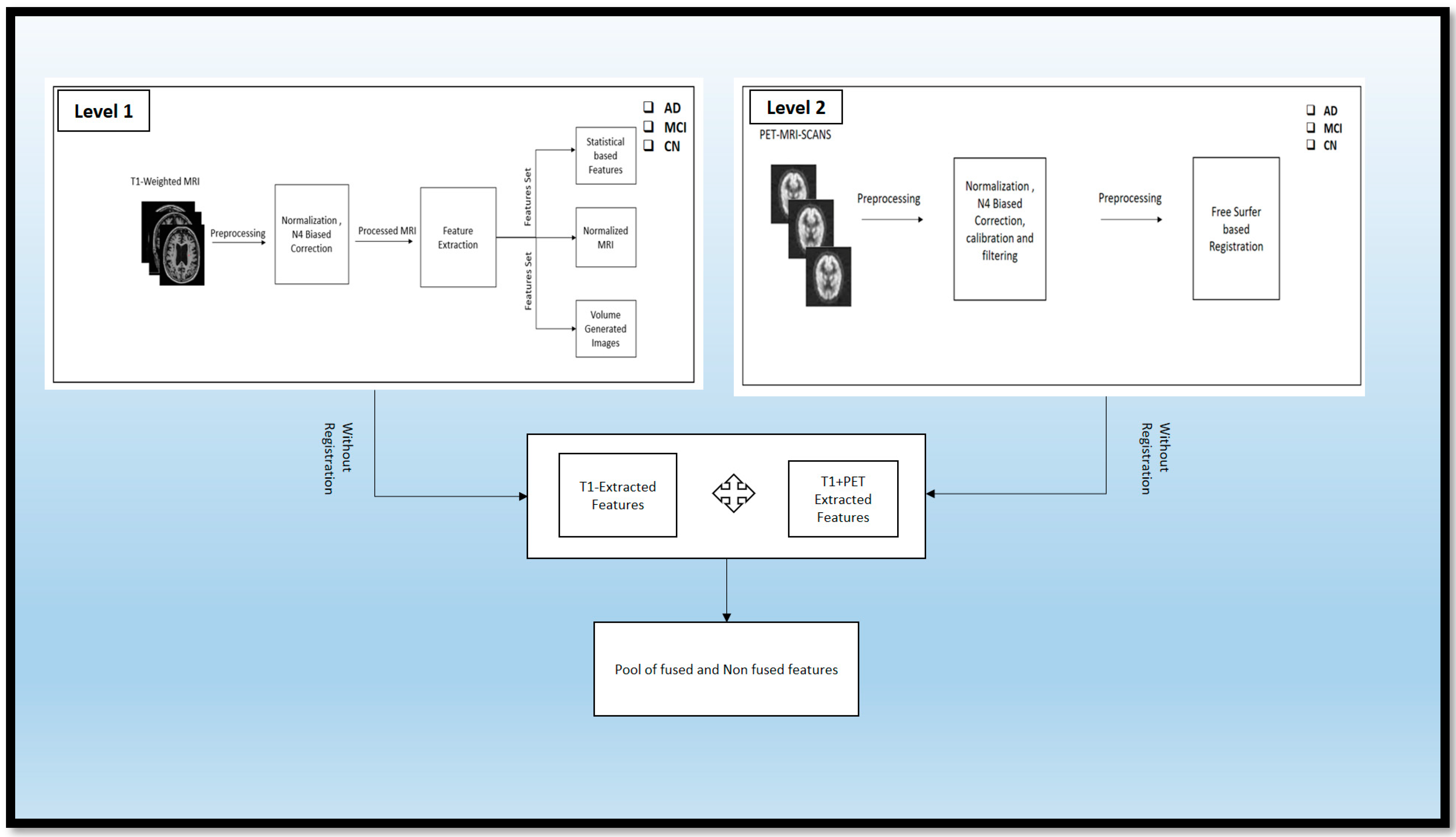
4.1. MRI SCANS

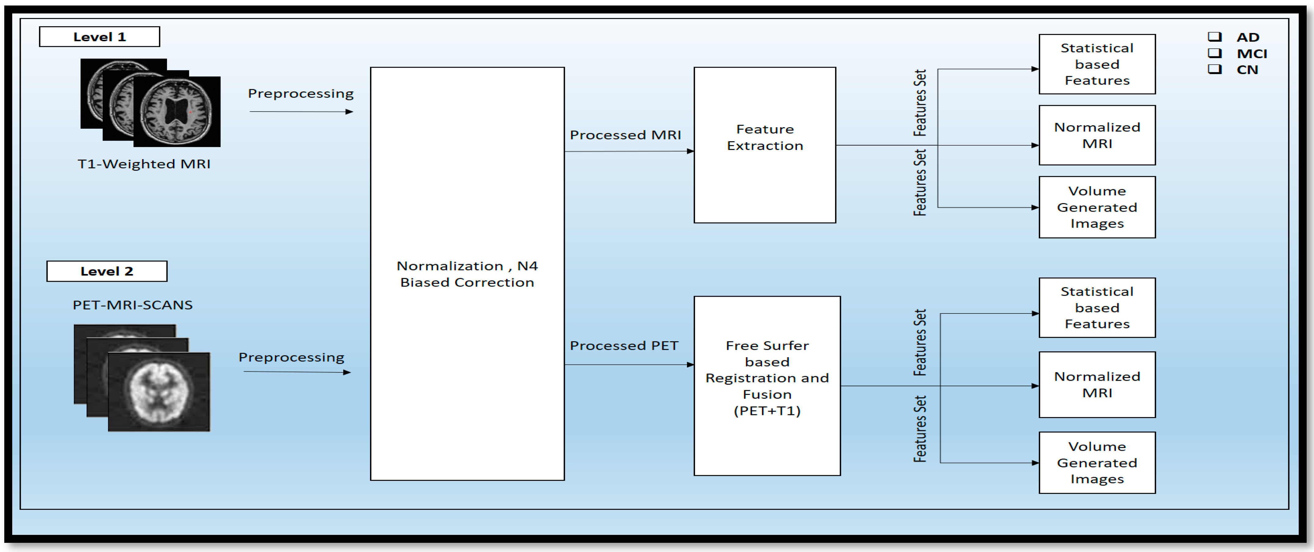
MRI scans were taken of these different classes: AD, MCI, and CN. These scans were raw scans. These scans came with high-rated features and unwanted features for disease diagnosis. So, to reduce the unwanted and noise-oriented elements, the different preprocessing steps, as given in Figure 3, were applied, including normalization and N4 bias correction. Then, the preprocessed MRI scans were processed for feature extraction using automatic pipeline methods and different statistical volume-generated features from the feature extraction method.

4.1.1. Normalization

The raw image taken from the ADNI data set was unprocessed. So, the normalization technique was applied in that data set to reduce unwanted features. This technique consists of adjusting the intensity range of a T1-weighted MRI image. It includes a proper visualization and understanding of the importance of the brain’s other regions that are affected by AD and its stages. This process is necessary to identify the anatomical features from the cortical area correctly. This formula involves the calculation of each pixel in the percentage range from 0 to 100 and mapping this range with the other pixels, which also normalizes the different intensities. The desired formulae for the calculation of normal image intensity are described in Equation (1):

$${\mathrm{N}}_{\mathrm{p}\mathrm{v}}=\frac{\left({\mathrm{P}}_{\mathrm{v}}-{\mathrm{M}}_{\mathrm{v}}\right)}{{\mathrm{M}}_{{\mathrm{a}}_{\mathrm{v}}}-{\mathrm{M}}_{\mathrm{v}}}$$

(1)

In Equation (1), ${\mathrm{N}}_{\mathrm{p}\mathrm{v}}$ defines the normal pixel intensity value, ${\mathrm{M}}_{\mathrm{v}}$ stands for the minimum pixel intensity and ${\mathrm{M}}_{{\mathrm{a}}_{\mathrm{v}}}$ describes the maximum pixel intensity.

4.1.2. N4 Biased Correction

After the normalization, the T1-weighted modality was processed using the N4 bias correction method to remove abnormalities from the different intensities of the MRI scanners. This preprocessing technique is an essential technique that consists of removing the various artifacts from the MRI scanners from the other version. This preprocessing method was applied to the MRI, PET, and DTI scans for better visualization. These corrections can be achieved through the formulae below, in Equation (2):

$${\mathrm{N}}_{\mathrm{P}\mathrm{v}}=\frac{1}{1+\exp \left(-\mathrm{k}\left({\mathrm{P}}_{\mathrm{v}}-\mathrm{c}\right)\right)}$$

(2)

In Equation (2), the normal pixel intensity value (${\mathrm{N}}_{\mathrm{P}\mathrm{v}}$) is calculated concerning the exponential constant and the pixel value attained from the different modalities of AD. $\mathrm{c}$ is the shift of the curve that receives the different parameter. The parameter k contains the slope of the curve. After the preprocessing, the processed T1-weighted MRI scans of the MCI, AD, and CN stages are fed as input to the feature extraction method, which utilizes the automatic pipeline method for the feature extraction.

4.1.3. Feature Extraction

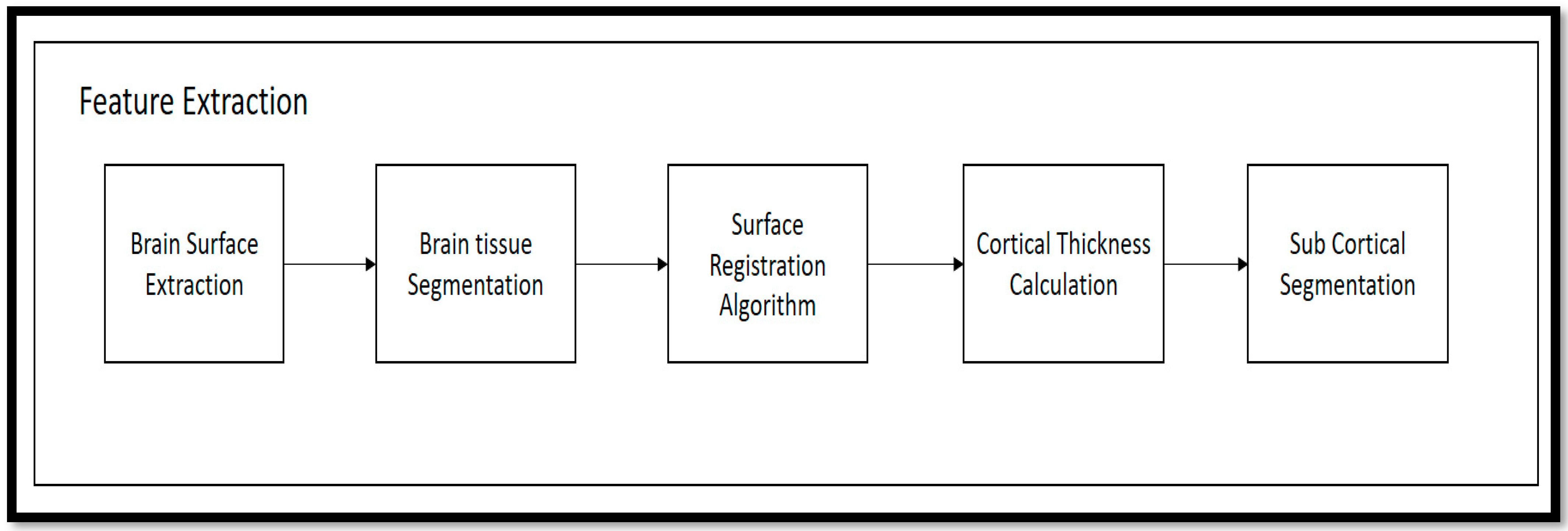
Following the preprocessing stage, the T1-weighted modalities undergo feature extraction methods. The Free Surfer methods are used for feature extraction, which consist of various fundamental algorithms that help to identify additional features in the brain region. This method uses the Brain Surface Extraction technique, which combines surface modeling and deformable models to identify the brain regions from MRI scans. The technique works on the principle of identifying curves that represent the different boundary regions of the brain. These boundaries are refined using other deformable methods available in the automatic pipeline method. Then, the Brain Tissue Segmentation technique uses a deformable model and MNI-template-based atlas to segment the different parts of the brain and identify areas with white matter (WM), grey matter (GM), and cerebrospinal fluid (CSF). The Surface Registration approach is employed to register the MRI images of the subject’s brain to a standard brain template and one another, to examine the regional brain volume and cortical thickness. This involves normalizing the intensities of the subject’s MRI scans using the standard template. The cortical thickness estimation is performed through surface modeling and the linear registration of the tissue segmentation results. To segment the brain into different subcortical structures such as the amygdala and Hp, atlas-based segmentation and intensity normalization are used. The entire process follows a professional and technical approach.

Then, after the completion of the execution shown in Figure 4, a different output is achieved in the form of folders, i.e., subject data, including anatomical image, cortical surfaces, WM segmentation, and GM segmentation. Statistical data were generated from the analysis of the brain data.

Algorithm 1 that describes transforming the raw T1-weighted data into processed T_1wMRIs through the N4 bias correction approach, which removes artifacts and normalizes the images for uniformity. Feature extraction techniques such as Brain Surface Extraction (T1_wMRI) and Brain Tissue Segmentation (T1_BSE) are applied to compare the different brain regions, followed by Surface Registration (T1_BTS) to identify other parts of the T1-weighted image. Cortical Thickness (T1_SR) is then calculated, and Sub-Cortical Registration (T1_CT) is implemented to produce volumetric shapes, constructed regions, and various cortical and subcortical brain regions in stat files. After completing level 1 experiments, similar preprocessing steps are taken to prepare the PET modality for the fusion process.

Algorithm 1 Feature Extraction from the Single Modality (T1-weighted MRI Scans)
1:	Input: Raw T1-weighted Image
2:	Output: Statistical-based features
3:	For I- = T T1wMRIs to n do
4:	{
5:	Normalization (T1wMRIsN4);
6:	{Npv = (Pv − Mv)/(Mav − Mv)}
7:	N4 Bias Correction(T1wMRIs);
8:	{N4v = (1/(1 + exp(−k ∗ (pv − c))))}
9:	return T1wMRI;
10:	}
11:	Then T1wMRI -> Processed to Free Surfer Method ()
12:	{
13:	Brain Surface Extraction (T1WMRI)
14:	Brain Tissue Segmentation (T1BSE)
15:	Surface Registration (T1BTS)
16:	Cortical Thickness (T1SR)
17:	Sub-Cortical Registration (T1CT)
18:	}
19:	End

4.2. PET SCANS

Before fusion, the preprocessing of the PET scans is one of the most important features. The preprocessing in the PET scans is used to remove noise, reduce artifacts, and improve the signal-to-noise ratio of the scans. The most common preprocessing techniques used for PET scans include N4 bias correction, normalization, and registration. Artifacts are reduced using techniques such as median filtering, which helps to remove artifacts by retaining the originality of the image. These artifacts are generally removed from the PET scans using the adaptive noise-filtering technique. In this technique, the noise-oriented input signal is found and then it is subtracted from the template signal by preserving the signal original form.

$$\mathrm{P}\mathrm{E}{\mathrm{T}}_{\mathrm{t}\mathrm{s}\mathrm{c}\mathrm{a}\mathrm{n}\mathrm{s}}=\left(1-\mathsf{\alpha }\right)\ast \mathrm{P}\mathrm{E}{\mathrm{T}}_{\mathrm{t}\mathrm{s}\mathrm{c}\mathrm{a}\mathrm{n}\mathrm{s}\mathrm{o}\mathrm{l}\mathrm{d}}+\mathsf{\alpha }\ast \mathrm{X}$$

(3)

In Equation (3), $\mathrm{P}\mathrm{E}{\mathrm{T}}_{\mathrm{t}\mathrm{s}\mathrm{c}\mathrm{a}\mathrm{n}\mathrm{s}}$ is the new noise level, $\mathrm{P}\mathrm{E}{\mathrm{T}}_{\mathrm{t}\mathrm{s}\mathrm{c}\mathrm{a}\mathrm{n}\mathrm{s}\mathrm{o}\mathrm{l}\mathrm{d}}$ is the old noise level, alpha is the adaption rate and x is the current noise sample.

Filtering involves using a low-pass or high-pass filter to remove high-frequency noise and artifacts Calibration is used to ensure that the intensities of the pixels are consistent across images. Normalization is used to adjust the intensities of pixels, so they are within a certain range. Finally, registration is used to align the images across multiple PET scans. This is conducted by using an adaptive noise-reduction technique, which helps to reduce noise without affecting the original image. Then the preprocessed PET scans are further supplied to the Free Surfer-based registration method.

Algorithm 2 contains the basic preprocessing approach which is contextual to PET scans. The PET scans are basically highly integrated into the features, but the vigilance of these features cannot be integrated through this individual modality. This modality requires a certain fusion approach with the T1-weighted image, to obtain the clear vision of the amyloid protein and the affected cortical region in the brain. These PET scans underwent the N4 bias correction methods, normalization and adaptive noise-filtering methods. These methods help in the fusion approach for the feature extraction of the PET scans.

Algorithm 2 Preprocessing approach in Single Modality (PETscans1)
1:	Input: Raw PETscans
2:	Output: Preprocessed PETscans
3:	For I- = PETscans to n do
4:	{
5:	N4 Bias Correction (PETscans1);
6:	$\{\mathrm{N}{4}_{\mathrm{v}}=(1/(1+\exp (-\mathrm{k}\ast$ (pv − c))))}
7:	Normalization (PETscans2);
8:	{Npv = (Pv − Mv)/(Mav − Mv)}
9:	Adaptive noise filtering
10:	PETtscans = (1 − α$)\ast$ PETtscansold + α $\ast$ x
11:	}

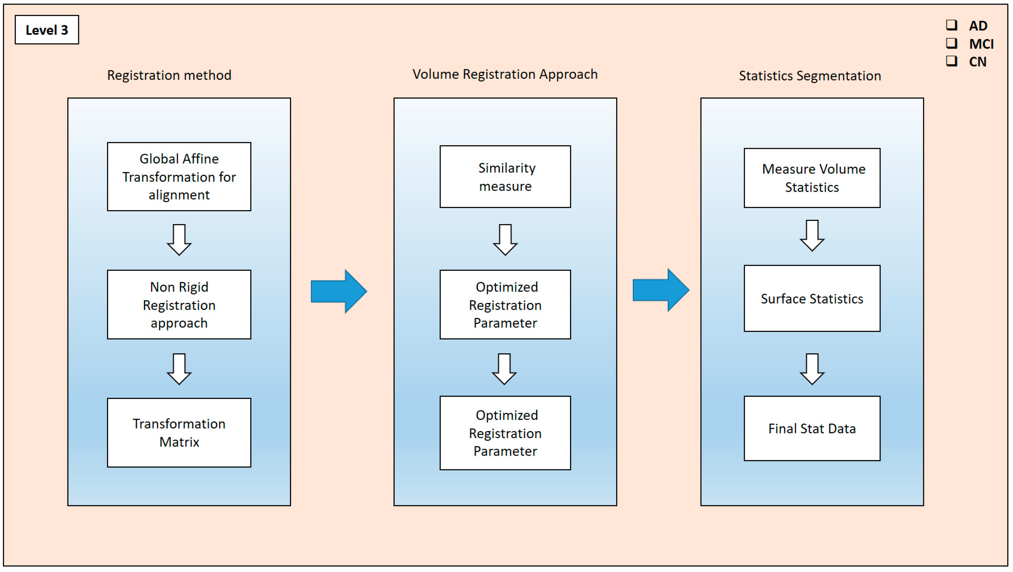
4.3. Multimodality Image Fusion

Image fusion is a technique in which the different modalities of images fuse to provide the hybrid set of features in Figure 5. Pixel-level, feature-level, and decision-level fusion are the basic types of image-fusion approaches in practice. In this process, we have chosen the pixel-level fusion approach to see the actual difference in the cortical region of AD and its different stages through these fused modalities. This helps reduce the noise level and provides a better resolution of the affected area of the brain region. The T1-weighted scans were processed through Free Surfer by the recon-all methods, which contain the pipeline of the different preprocessing steps and help to evaluate the significant features—volume, area, mean, and others—of the different cortical regions the brain. The T1 and PET scans are taken using a register method, where a global affine transformation is implemented for alignment. This transformation method produces a better comparison and study of these modalities, which can be enriched with the GM, WM, cortical thickness, and presence in the neuro region. This was operated using the three translations and aligned adaptation approaches. After the registration method, the mutual characteristics of these modalities required us to determine the similarity between the two scans. After the fusion of these two scans, the volume registration approach wraps PET and MRI images by translating the source volume to the target volume’s space. To align these volumes and bring them into a unified space, the mri_vol2vol method establishes their transformation matrix. Subsequently, the similarity measure between the two modalities was analyzed.

The fused (PET and MRI) images’ similarity measures were optimized through the different registered parameters. They were also fine-tuned through this approach. These recorded parameters were taken into account when creating the transformation matrix. This matrix calculates the segmented features via the stat segmentation approach from the Free Surfer method. Hence, the volume statistics were measured in the different regions, and using the additional stat data, the calculations were performed for this approach. These stat data were calculated for the specific ROI in the brain, such as the frontal lobes, temporal lobes, occipital lobes, and cerebellum, as well as subcortical structures such as the Hp, amygdala, thalamus, and basal ganglia. Hence, these generations of the different stats contain cortical thickness, surface area, folding index, curvature, mean curvature, and cortical volume.

Algorithm 3 that is fusion of the T1 scans and PET modality. Here, in this table, we first applied the bb-registration methods for performing the registration, including global affine transformation and non-rigid transformation, and then we returned the registered modality. Then, these fused modalities went to volume-to-volume mapping, where they were altered in the similarity measurement and correlation matrix, and we returned the matrix. From the correlations matrix, the stat features were extracted, including the volume statistics and surface statistics for the variation in the classification of AD, MCI and CN classes.

Algorithm 3 Algorithm for Fusion Dual Modality (PETscans + T1scans)
1:	Input: Preprocessed PETscans and T1scans
2:	Output: Stat_data_neuroregion
3:	for I = PETscans and T1scans to n do
4:	Register_method              {
5:			Global affine transformation (PETscans + T1scans);
6:			Non-Rigid Registration (PT1rscans);
7:			Return Matrix (NRPETscans + NRT1scans);
8:			}
9:	Volume to Volume Mapping                   {
10:			Similarity Measure (NRPETscans + NRT1scans)
11:			Correlation Matrix (NRPETscans + NRT1scans) optimized parameters
12:			Return Matrix ((NRPETscans + NRT1scans) optimized parameters
13:			}
14:	Stats Extraction From Output of v to v Mapping      {
15:			Volume Statistics (((NRPETscans + NRT1scans) optimized parameters))
16:			Surface Statistics ((((NRPETscans + NRT1scans) optimized parameters))
17:			Return Stat Data (((((NRPETscans + NRT1scans) optimized parameters)))
18:			}
19:	end

4.4. Feature-Level Fusion

For our feature-level fusion, we extracted the relevant features from T1-MRI scans, which include calculation of the volume, area, white matter, curving, folding, Gaussian curve, thickness, and folding from the different cortical regions of the brain. In the same way, after fusion (T1 + PET), we extracted the features from the combined modality and compiled them into one stat file for further classification. Before applying these combined features, we used the correlation and drop-out techniques for the removal of unwanted features before the selection of features. We applied Binary- and Multi Class-level classification for the intended classes: AD, MCI, CN. The whole process is represented in Figure 6.

CS_R = [F_T₁, F_FNF_R]

(4)

Let n_t1 be the number of features extracted from the T1 modality (F_T₁) and n_fnfr be the number of features extracted from the FNFR modality (F_FNF_R). If we have m samples, then the matrix representation of the CSR will be an m x (n_t₁ + n_fnfr) matrix, denoted as CSR_mat:

$$\mathrm{C}\mathrm{S}\mathrm{R}\_\mathrm{m}\mathrm{a}\mathrm{t}=\left|\begin{array}{c}\begin{array}{cc}{F}_{T{1}_1}& F_{FNF{R}_1}\\ F_{T{1}_2}& F_{FNF{R}_2}\end{array}\\ ⋮\\ \begin{array}{cc}{F}_{T{1}_m}& F_{FNF{R}_m}\end{array}\end{array}\right|$$

(5)

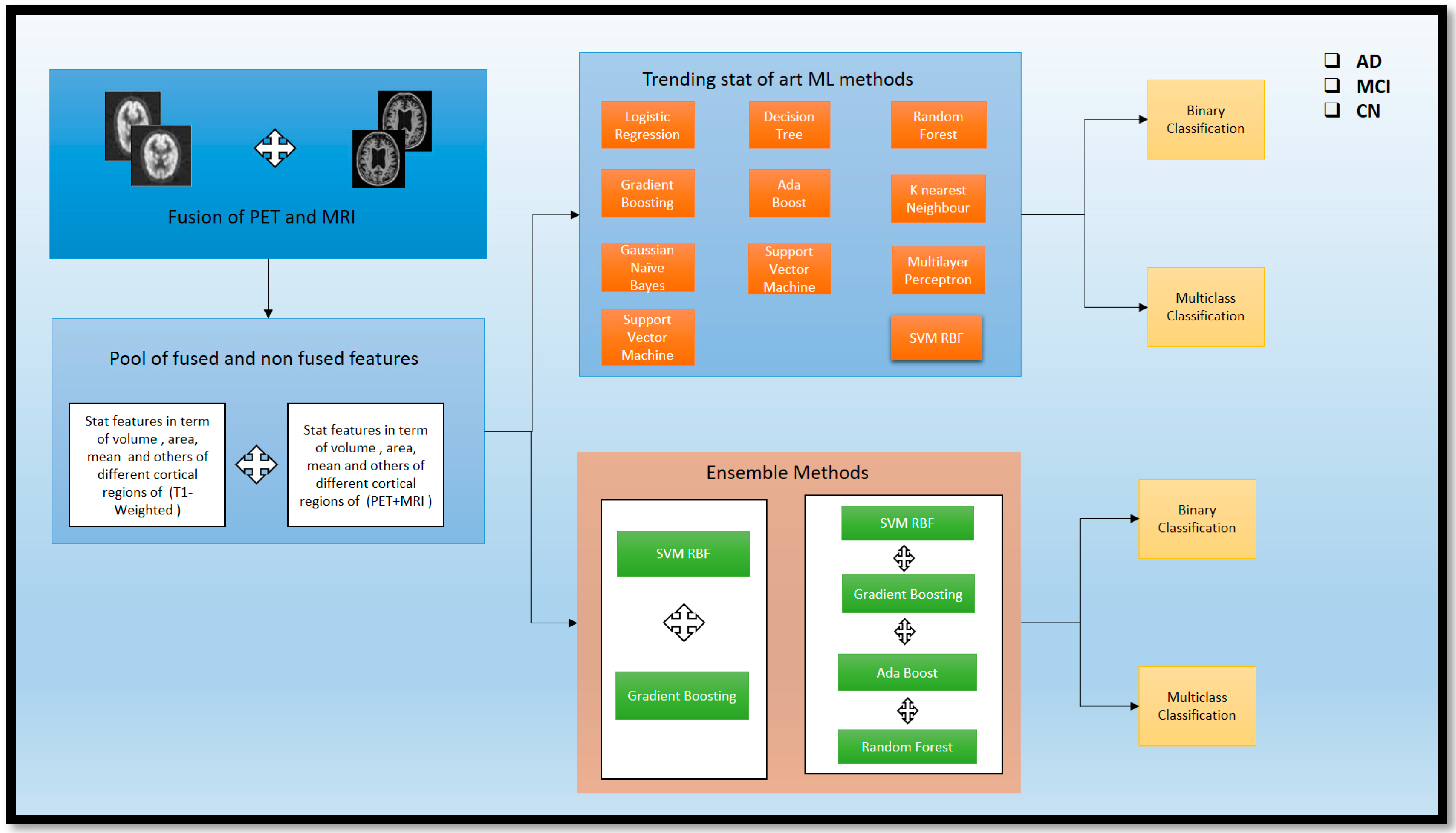
4.5. ML and EL Models

ML methods are currently trending as essential techniques for classifying different stages of AD. However, using the ensemble technique for validating results is a novel approach that has yet to be explored in the trending ML methods for classifying AD, MCI, and CN individuals. Therefore, both approaches were used in our study, utilizing the latest trending ML approach, as shown in Figure 6. We ensembled from those methods to validate the classification (A_cc) of AD, MCI, and CN. We used a feature-fusion approach to obtain a pool of fused and non-fused features, including the area, maximum, mean, number of vertices, and number of voxels, standard deviation, and volume from the fused (PET and MRI) scans. Additionally, we considered the segmented volume, mean, and area from the segmented region of the non-fused scans. These features were then passed through the ML and EL approaches for further AD, MCI, and CN classification. The process is described in detail in Figure 7.

4.6. ML Methods

There are some current ML methods that are traditionally used for the classification of AD and its subtypes. Here, recent methods have been used for the category. Logistic Regression (LR) is the statistical technique employed for the Binary type. A Decision Tree (DT) model resembles a flowchart and divides data depending on the feature values. Random Forest (RF) is a collection of Decision Trees that reduces overfitting. Gradient Boosting (GB) is an iterative approach that merges weak learners to enhance prediction. Ada Boost (AB) is a boosting algorithm that changes sample weights to improve classifier performance. K-Nearest Neighbor (KNN) is an instance-based technique that categorizes data based on the majority vote of its nearest neighbors. Gaussian Naive Bayes (GNB) is a probabilistic classifier based on Bayes’ theorem with an assumption of Gaussian distribution. Support Vector Machine (SVM) is a technique that determines the best decision boundary between classes. Multi-layer Perceptron (MLP) is a neural network that learns non-linear relationships in a feedforward manner. Lastly, Support Vector Machine RBF (SVM-RBF) is an SVM that incorporates a Radial Basis Function Kernel to allow for non-linear decision boundaries. LR uses multi_class = ‘auto’ for automatic Multi Class strategy selection; DT uses default settings; SVM uses a linear kernel, C = 0.9 for regularization, RF uses default settings; GB and AB use default parameters; KNN uses three nearest neighbors; GNB uses a default parameter; MLP uses two hidden layers, ReLU activation, and the Adam solver; and SVM RBF uses an RBF kernel, gamma = 0.9, and C = 1. Hence, these are the parameters used for both the Binary and Multi Class for AD.

4.7. El Methods

To see the effectiveness reached in the (A_cc), we tried this ensemble of different traditional ML models. First, we combined Gradient Boosting (GB) and Support Vector Machine with Radial Basis Function Kernel (SVM_RBF) to create an ensemble method (SVM_RBF + GB) to classify Alzheimer’s disease (AD) subtypes. The voting classifier is an ensemble learning algorithm that improves (A_cc) and stability by leveraging diversity among the base models. The voting classifier ensemble algorithm is used with the output of a GB classifier and an SVM with an RBF kernel. It is a ‘hard’ voting approach, selecting the class with the most votes from the base models. The SVM was adopted with the same parameter as a decision boundary flexibility, C = 1 was used to enable regularization and generalization, and Multi Class classification was performed. GB improves prediction (A_cc) by iteratively refining the weak metrics data, while SVM_RBF excels in the classification removal of nonlinear data, which is included stat data part. Hence, the combination of these models provides a better classification for the Multi Class of AD and its subtypes.

Similarly, we adopted this ensemble approach for Binary Class classification. Here, we used the four models so the ensemble performed better in the Binary Class, especially in the (AD vs. MCI). The (SVM_RBF + AB + GB + RF) is for the Binary classification of AD and subtypes of AD. The model, which is a combination of four different classifiers, includes specific parameters for each one. One of the classifiers is an SVM with an RBF kernel, with gamma = 0.9 to control how the decision boundary is shaped, a regularization parameter of C = 1, and decision_function_shape = ‘ovr’ for Multi Class classification. Two other classifiers use default parameters for AB classifier () and GB classifier (). The fourth classifier, RF, utilizes RF classifier () with a criterion of ‘gini’ and n_estimators = 100, which determine the number transit in the data. This can enrich the classifier with better performance for classifying AD and its subtypes. Consequently, after implementing these techniques, significant findings were observed for identifying AD and its various stages. A detailed discussion is presented in Section 5.

5. Result Analysis and Discussion

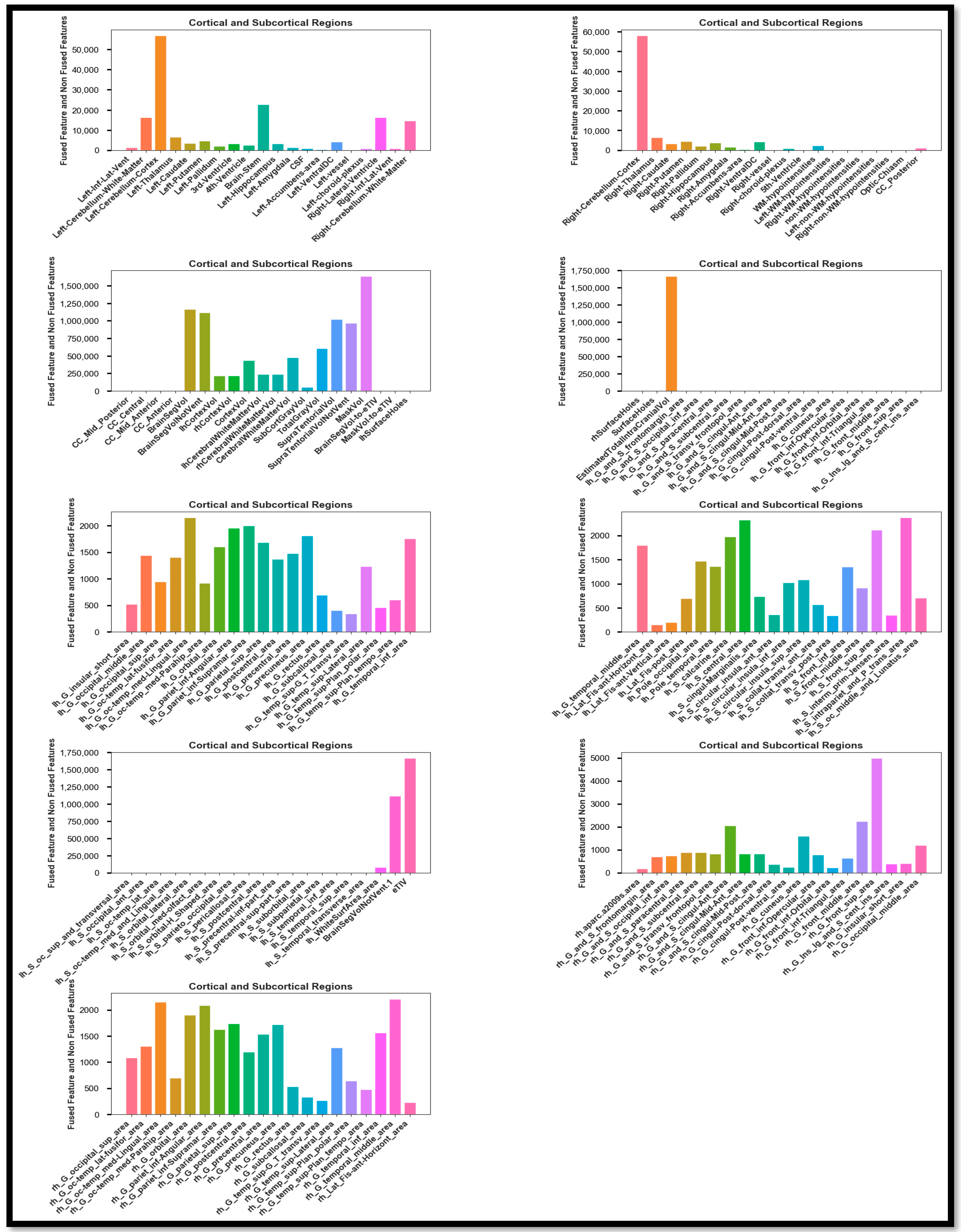
After the fusion of the features extracted from the fused PET and T1-weighted modalities and the non-fused modalities, the high-intensity and noise-integrated features were in the generated stat file. These features required regress preprocessing before the feature selection. For the different features, normalization, correlation, scaling, and feature drop-out techniques were applied to detect AD and its stages. First, this study uses the correlation approach to filter out the relevant data whose impact is more significant than 0.9. This procedure already normalized these remaining features. The feature selection method ANOVA F-value and the RF technique were used for feature selection. Hence, the selected features were obtained as shown in Figure 8. This feature set contains information about the different forms of statistical calculation of the other cortical regions of the brain. Hence, after the feature selection, these feature sets passed through various trending learning techniques for classifying AD and its stages. These techniques include LR, DT, SVM, RF, GB, AB, KNN, GNB, MLP, and SVM_RBF for the Binary and Multi Class classification of AD, MCI, and CN, and similarly, the ensemble methods (SVM_RBF + GB) and (SVM_RBF + AB + GB + RF). Section 5.1 covers Experiment 1, which involves Binary classification using ML and EL techniques. Section 5.2 details Experiment 2, where Multi Class classification is performed among AD, MCI, and CN classes. The same EL and ML methods are also used here. These classifications are conducted using different performance metrics in terms of (A_cc), precision (P_rec), recall (R_rec) achieved, and F1 score (F1_sco).

5.1. Experiment 1

Experiment 1 involved performing Binary Class classification on three classes from the Alzheimer’s data set (AD, MCI, and CN). The results of the Binary Class, by applying these standalone learning and EL methods, are described in

Table 2. The results achieved from the different trending methods and performing the Binary classification (MCI vs. CN).

Model	(Acc)	(Prec)	(Rrec)	(F1sco)
LR	98	98	98	98
DT	98	98	98	98
SVM	99	99	99	99
RF	98	99	99	99
GB	97	99	99	99
AB	96	99	99	99
KNN	74	79	73	72
GNB	81	81	81	81
MLP	75	84	75	74

.

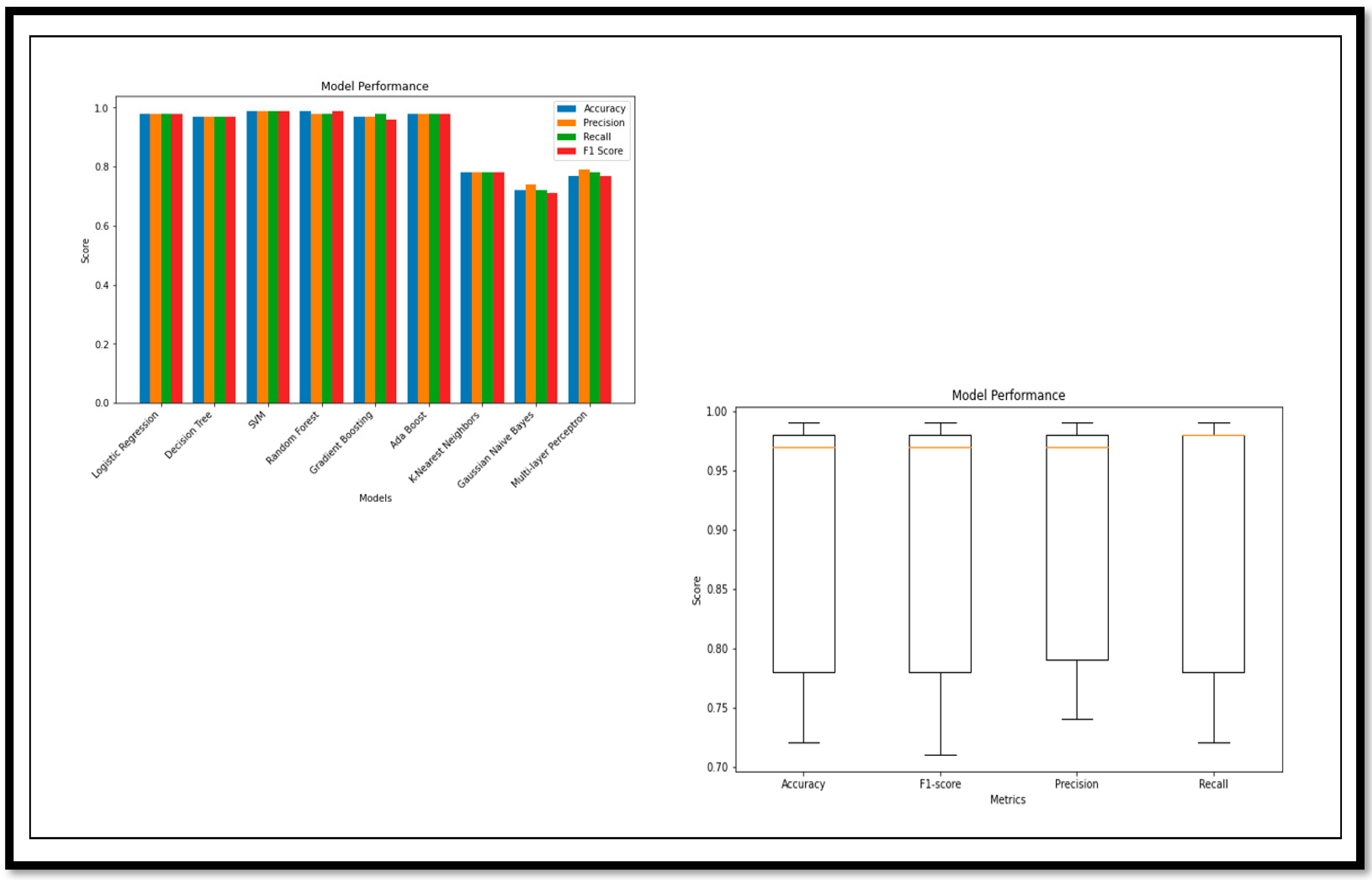
Among these models, the SVM has the highest A_cc (98), P_rec (99), R_rec (99), and F1_sco (99), indicating that it performs the best overall. The other models also perform relatively well, with high A_cc, P_rec, R_rec, and F1_sco scores, ranging from 98 to 99. However, KNN and MLP models have relatively lower performance scores. In the classification of MCI vs. 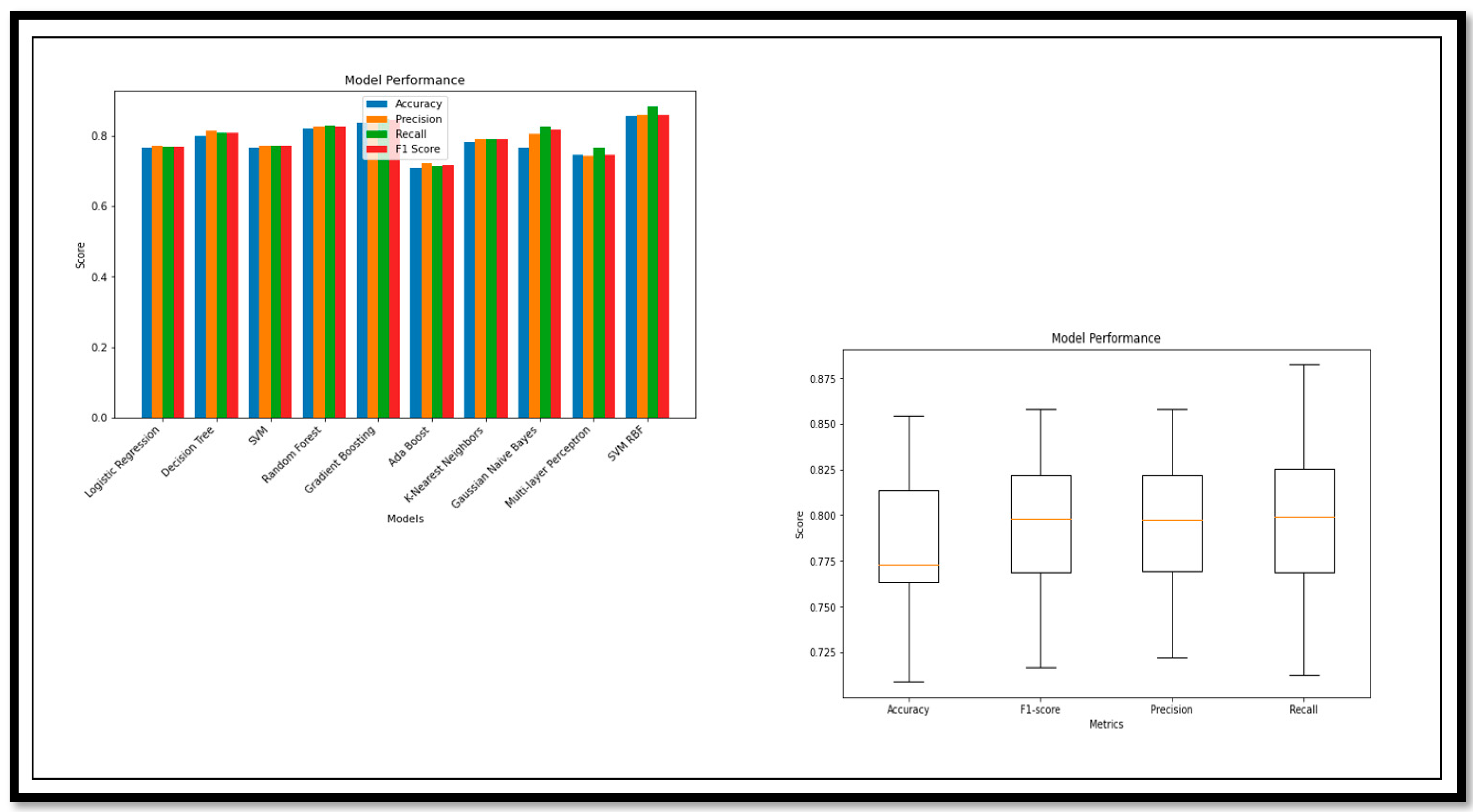CN, we did not use the ensemble method; the adequate (A_cc) was achieved through standalone ML methods. The performance analysis is described using the graph and the box plot of all the models for this classification in Figure 9.

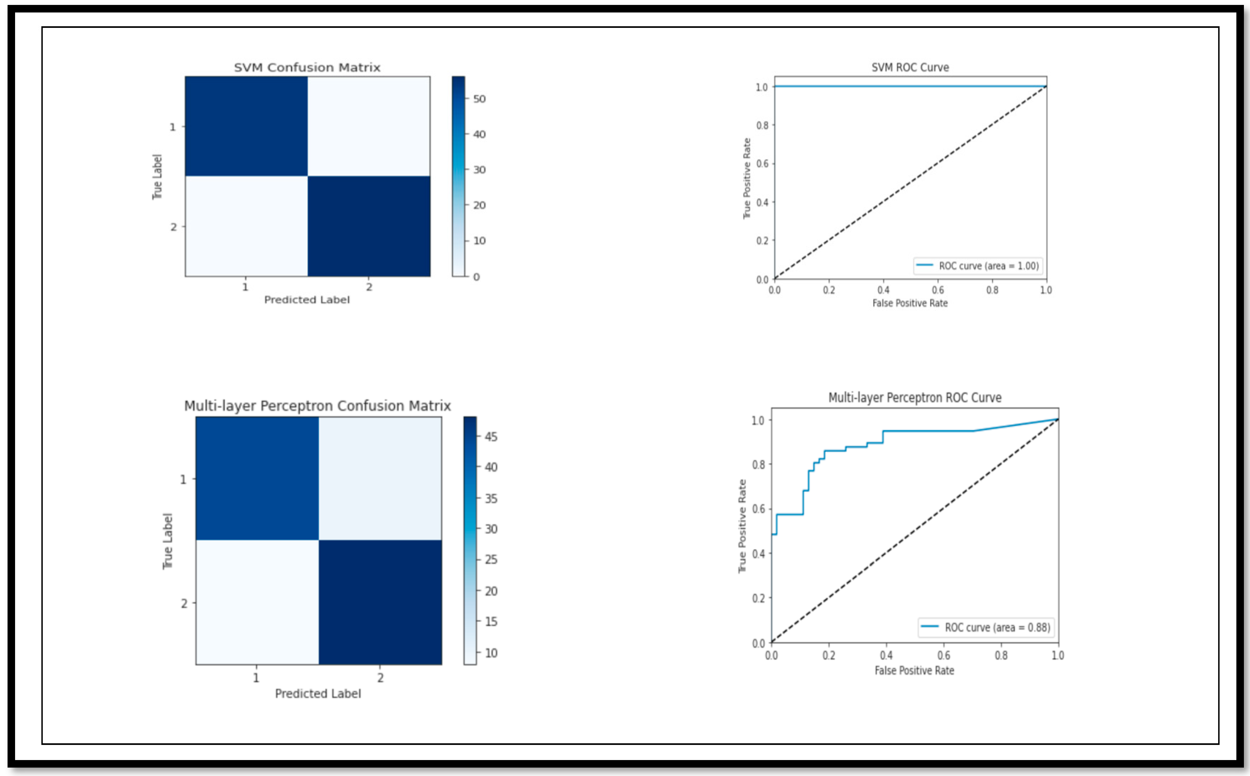
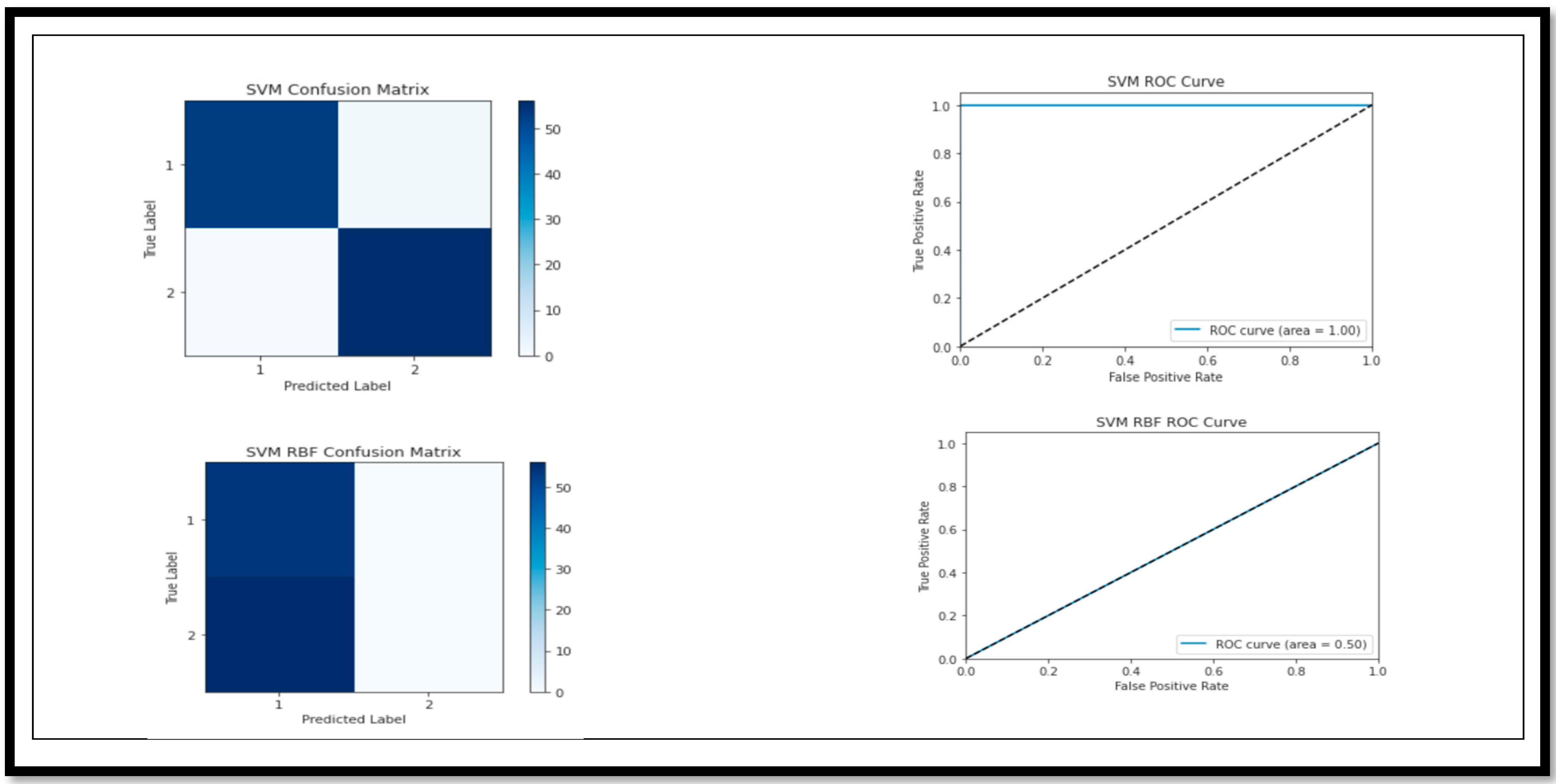
The model break down, on the basis of the performance parameters for (MCI vs. CN), is shown below. The ROC curve and confusion matrix of the model with high and low (A_cc) are shown in Figure 10.

Again, we performed the classification for the other classes, such as AD vs. MCI. The conversion of MCI to AD always has challenges in the classification. These challenges increase due to the similarity in some of the features, where the classification model is unable to find the difference in the comparison. Here, in this classification, we used standalone methods and ensemble methods.

Table 3. The results achieved by the different ML models for the Binary Class (AD vs. MCI).

Model	(Acc)	(Prec)	(Rrec)	(F1sco)
LR	72.97	74.55	72.97	72.89
DT	81.08	81.25	81.08	81.11
SVM	72.97	73.48	72.97	73.01
RF	86.49	86.65	86.49	86.51
GB	89.19	89.19	89.19	89.19
AB	89.19	89.57	89.19	89.11
KNN	89.19	89.74	89.19	89.21
GB	54.05	77.03	54.05	44.73
MLP	54.05	29.22	54.05	37.93
SVM RBF	86.49	86.53	86.49	86.45
(SVM_RBF + AB + GB + RF)	91.89	91.98	91.89	91.87

below describes the detailed results, which were obtained after applying all these models.

The ensemble method (SVM_RBF + AB + GB + RF) has the highest (A_cc) 91.89, (P_rec) 91.98, (R_rec) 91.89, and (F1_sco) 91.87, indicating that it has the best performance value as compared to the others. AB, GB, KNN with an (A_cc) of 89.19 and (P_rec), (R_rec), and (F1_sco) close to 89, is quite close to a good performance. The models, including LR, DT, SVM, GB, MLP, have relatively reduced (A_cc), (P_rec), (R_rec), and (F1_sco) levels. The ensemble and RF, GB, and AB models show an acceptable (A_cc), while other models such as LR, DT, SVM, GB, and MLP are lacking concerning the conversion of MCI to AD. The model break down, on the basis of the performance parameters for the classification of (AD vs. MCI), is in Figure 11.

The ROC curve and confusion matrix of the model with high and low (A_cc) (AD vs. MCI) are shown in Figure 12.

In the previous classification, we observed that the conversion of AD vs. MCI does not provide the greater A_cc as compared to the CN vs. MCI. An adequate (A_cc) is achieved through the ensemble model of 91. Now, again, we performed the classification of the pure AD class vs. the CN class. The performance of these different models was acquired and the results are described in

Table 4. Describes the results achieved by the different ML models for the Binary Class (AD vs. CN).

Model	(Acc)	(Prec)	(Rrec)	(F1sco)
LR	98	98	98	98
DT	97	97	97	97
SVM	99	99	99	99
RF	99	98	98	99
GB	97	97	98	96
AB	98	98	98	98
KNN	78	78	78	78
GNB	72	74	72	71
MLP	77	79	78	77

.

The SVM model has the highest (A_cc) (99), (P_rec) (99), (R_rec) (99), and (F1_sco) (99), indicating that it performs the best overall. The RF and AB models also have high (A_cc), (P_rec), (R_rec) and (F1_sco), with scores of 99 and 98, respectively. The LR, DT, GB, KNN, GNB, and MLP models have lower performance metrics in comparison to the other models. The performance analysis using a graph and a box plot of all the models for these classifications is described in Figure 13.

The model break down, on the basis of the performance parameters for the classification of (AD vs. CN), is shown below. The ROC curve and confusion matrix of the highest (A_cc) and lower (A_cc) achieved by the model for the classification are shown in Figure 14.

Hence, after seeing the performance of the classifications of all the classes (AD, MCI and CN), Binary Class detection has the maximum (A_cc) of 99% using the SVM model. AD vs. MCI classification also shows a sustainable (A_cc) as compared to previous research trends. After the Binary Class, we performed Multi Class detection for the detection of AD and its different stages.

5.2. Experiment 2

Since Binary Class classification was conducted and an adequate (A_cc) was achieved using the classification models, we could again apply this model for Multi class and see the performance of this model in this scenario.

Table 5. Describes the results achieved by the different ML models for the Binary Class (AD vs. MCI vs. CN).

Model	(Acc)	(Prec)	(Rrec)	(F1sco)
LR	58.18	61.41	58.18	57.27
DT	82.73	83.10	82.73	82.88
SVM	59.09	65.12	59.09	54.34
RF	86.36	87.57	86.36	86.51
GB	93.64	93.71	93.64	93.66
AB	71.82	73.45	71.82	72.24
KNN	86.36	89.78	86.36	86.45
GNB	65.45	69.16	65.45	65.25
MLP	61.82	65.23	61.82	60.71
SVM_RBF	91.82	93.00	91.82	91.90
GB + SVM + RBF	96.36	97.42	96.36	96.36

describes the detailed results, which were obtained after applying all these models (AD vs. MCI vs. CN).

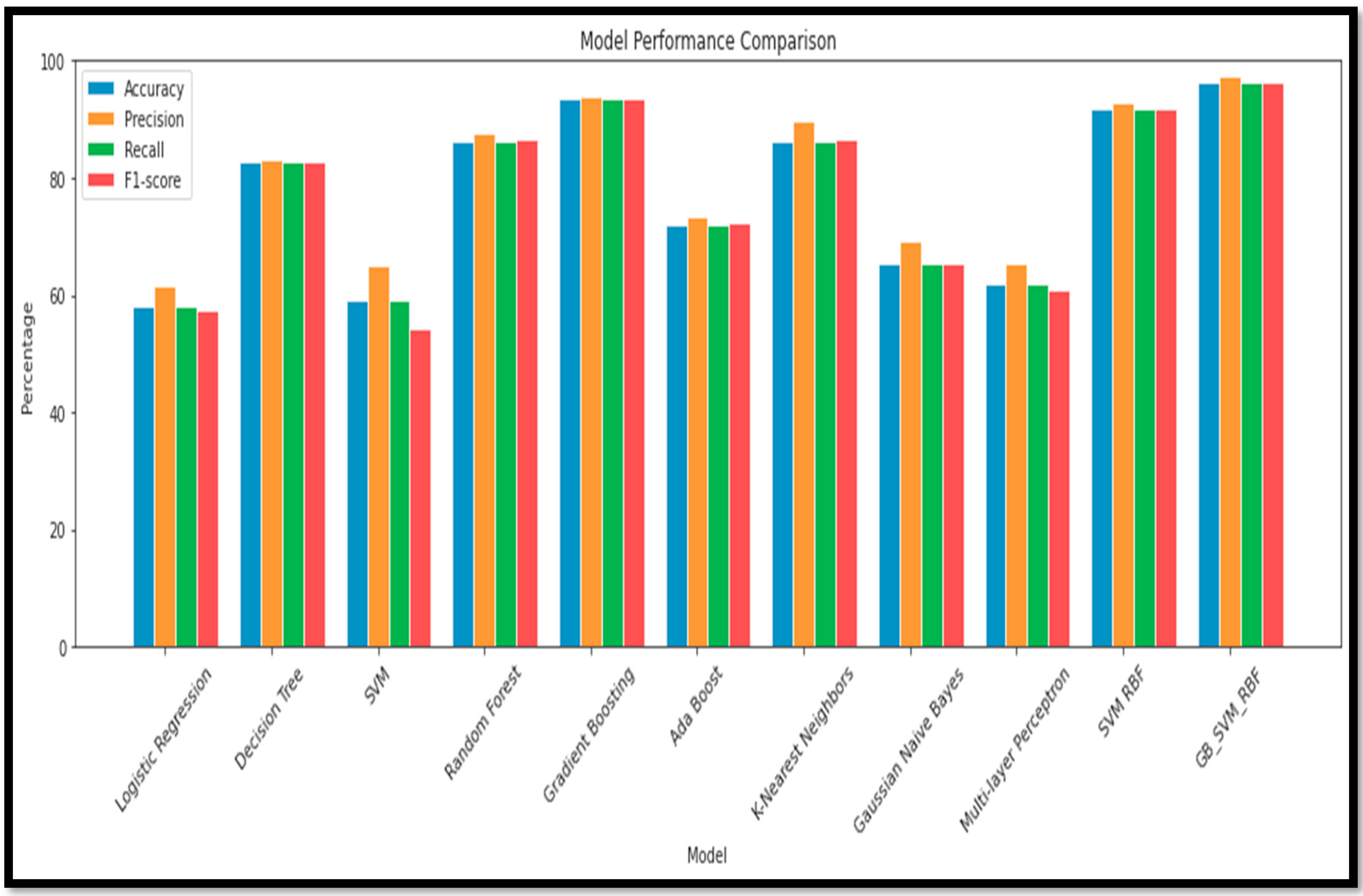
Based on the results, the ensemble model has lots of potential for the m=Multi Class classification of AD and its subtypes. There was a sustainable (A_cc) achieved in the Multi Class through the ensemble model as compared to standalone learning methods. The ensemble model (GB_SVM_RBF) has the highest (A_cc), with 96.36% (A_cc) and an (F1_sco) of 96.36%. In contrast, the Logistic Regression model has the second-lowest performance in both (A_cc) (58.18%) and (F1_sco) (57.27%). Other models, such as (RF), (GB), and (SVM_RBF) also demonstrate strong performance, while models such as (GNB) and (MLP) are less accurate and have lower (F1_sco) levels. The performance analysis, using a graph and a box plot, of all the models for these classifications is described in Figure 15.

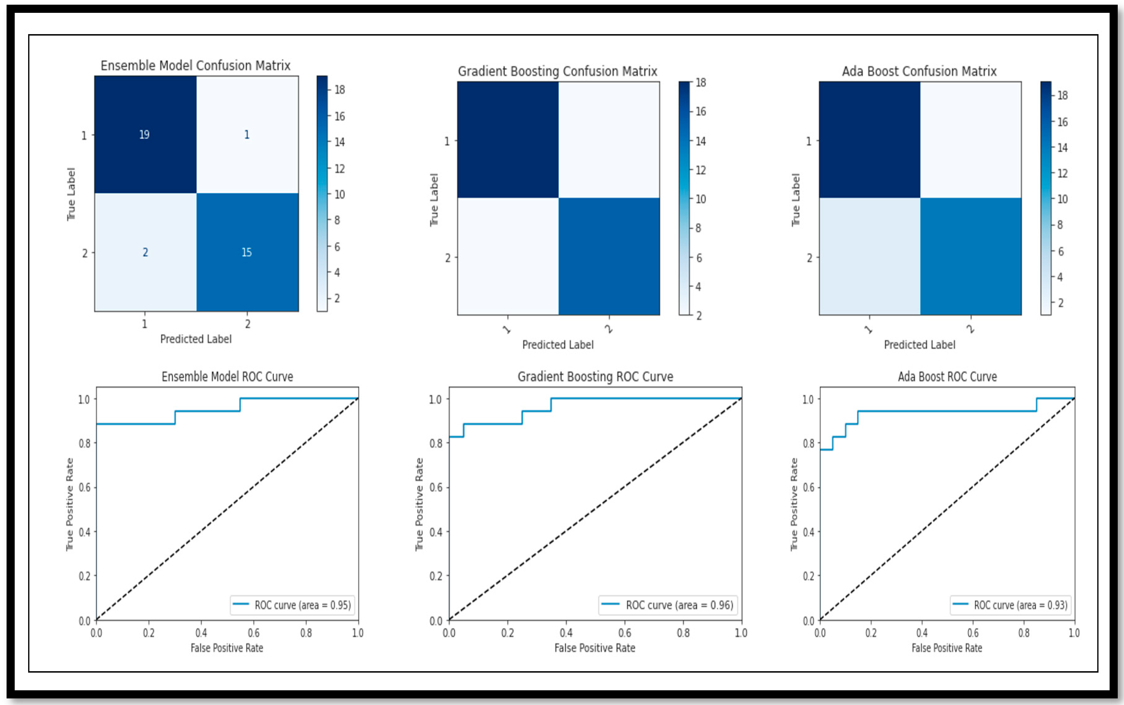
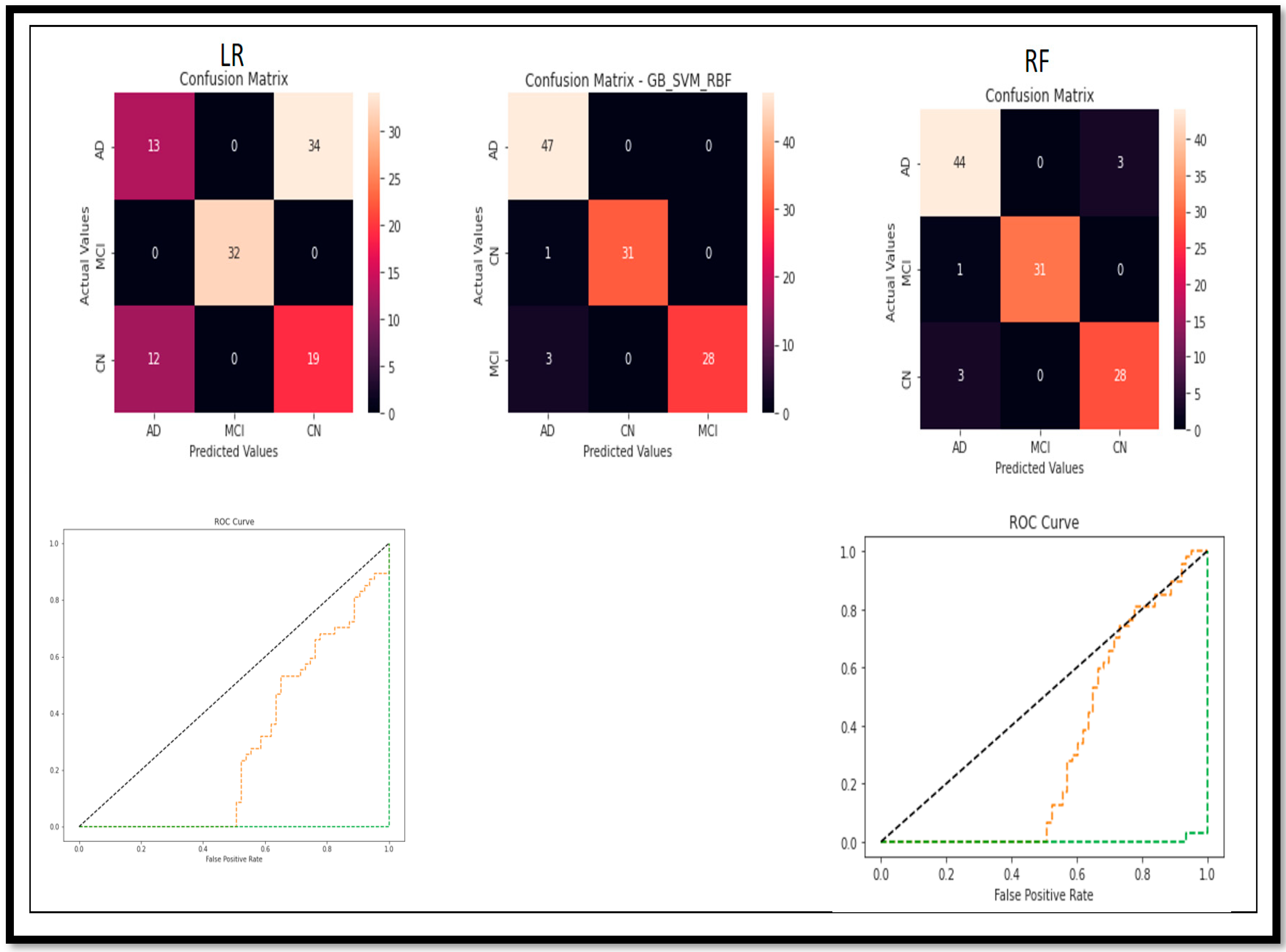
Following the evaluation of performance metrics and model performance for all models, we also examined the Confusion Matrix and ROC curve for each model in relation to the results obtained for (BC) (AD vs. MCI vs. CN) (Figure 16).

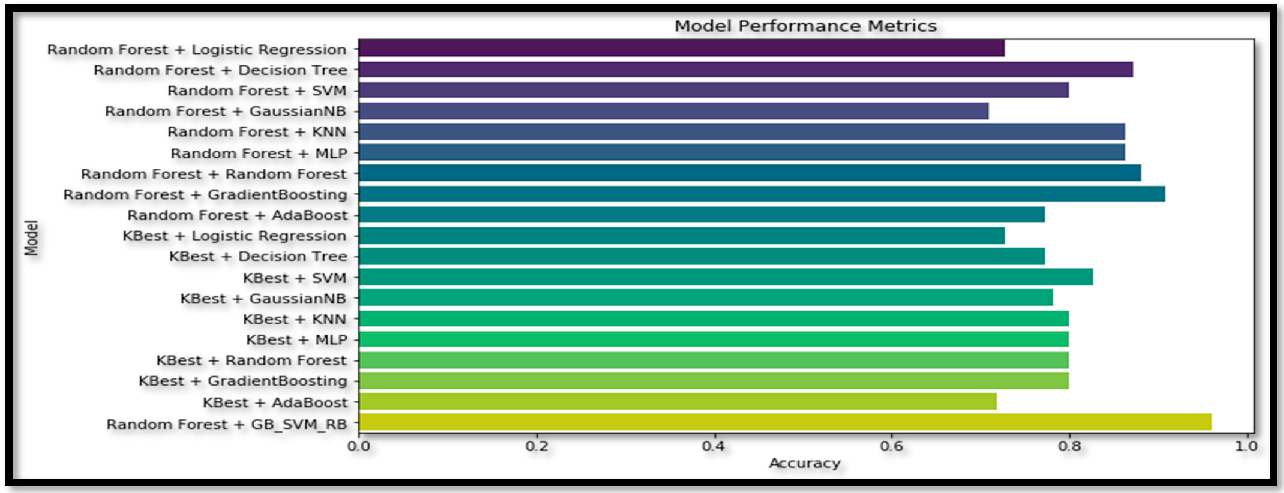
To further validate our study, we employed various feature selection (Random Forest and KBest) and classification techniques and observed the differing results upon applying these models. When conducting an ablation study concerning feature selection methods and classification models, the ensemble model consistently demonstrated superior accuracy compared to the other models utilized, shown in

Table 6. Describes the ablation study of the different ML and Ensemble models for the Multi Class (AD vs. MCI vs. CN).

Model	(Acc)
RF + LR	72.73
RF + DT	87.27
RF + SVM	80.00
RF + GNB	70.91
RF + KNN	86.36
RF + MLP	86.36
RF + RF	88.18
RF + GB	90.91
RF + AB	77.27
KBest + LR	72.73
KBest + DT	77.27
KBest + SVM	82.73
KBest + GNB	78.18
KBest + KNN	80.00
KBest + MLP	80.00
KBest + RF	80.00
KBest + GB	80.00
KBest + AV	71.82
GB_SVM_RBF	96

.

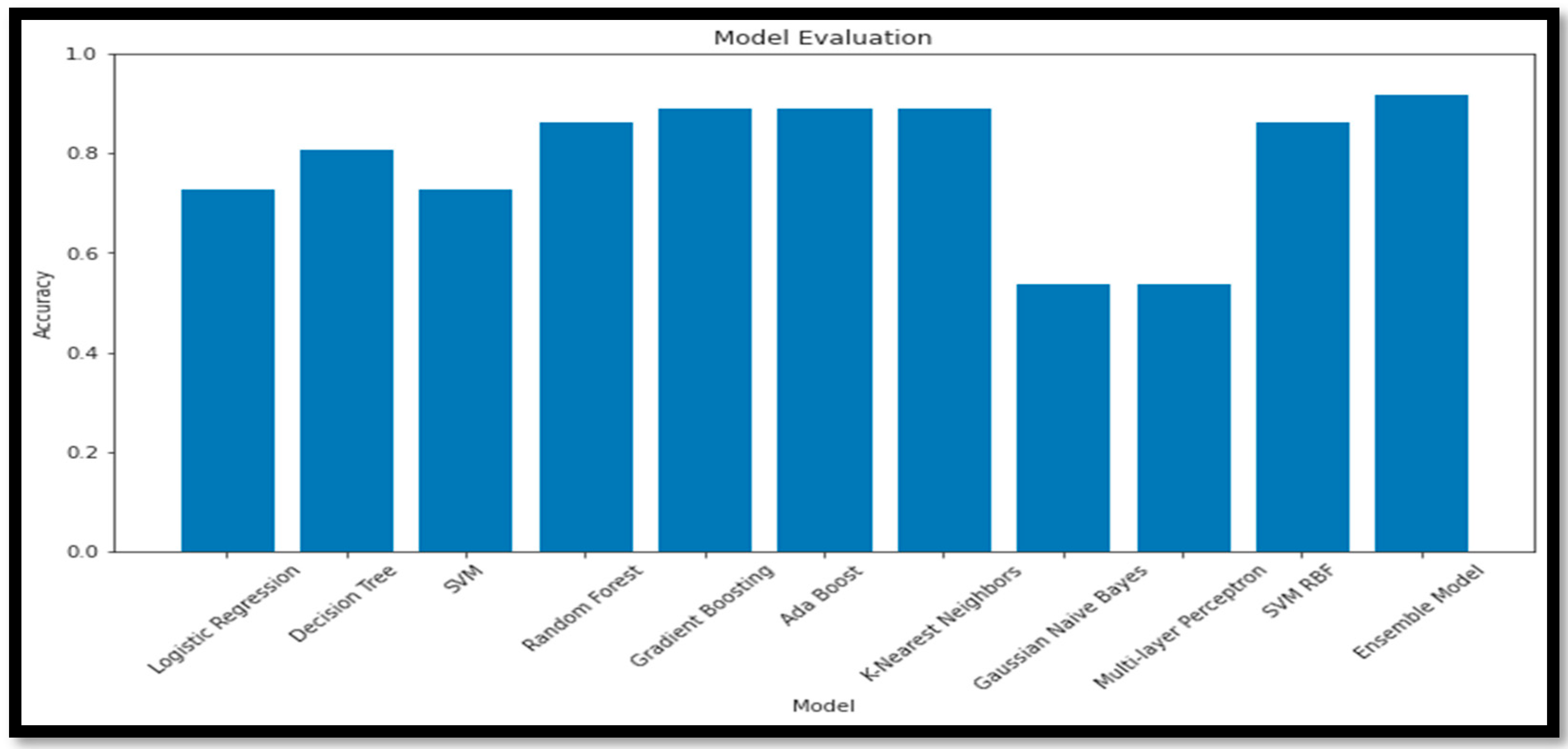
Table 6 presents the accuracy (A_cc) of various combinations of feature selection methods and classification models. The ensemble model ‘RF + GB’ achieves the highest accuracy (90.91%) among the non-ensemble models. The original ensemble model, ‘GB_SVM_RBF’, outperforms all the other models, with an accuracy of 96%. Comparing the feature selection methods, models using ‘RF’ generally achieve higher accuracy than those using ‘KBest‘. Among the classifiers, ‘DT’, ‘KNN’, and ‘MLP’ consistently yield relatively high accuracy scores when combined with different feature selection methods. The ‘GNB’ and ‘AB’ classifiers result in lower accuracy scores in most cases, indicating they may not be the most suitable classifiers for this data set. The ensemble model ‘GB_SVM_RBF’ demonstrates the best performance, and utilizing the ‘RF’ feature selection method yields superior results to the ‘KBest’ method. The plot for this study is represented in Figure 17.

The cumulative (A_cc) comparison of the Binary Class and Multi Class classes of the AD with respect to the different models is shown in Figure 18.

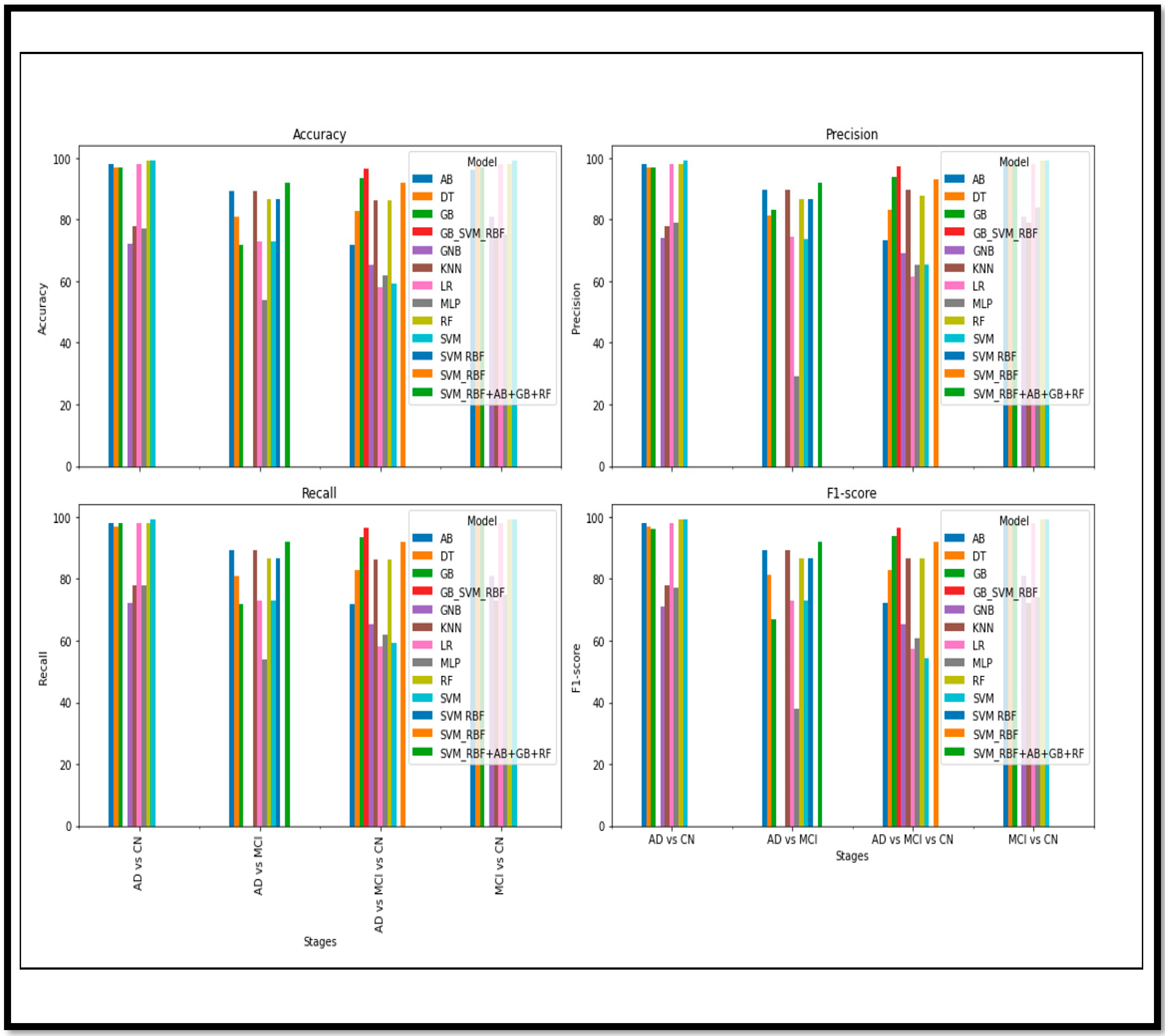
Regarding the fusion of the features and images, the results have effectively shown progress in detecting AD and its stages. The fusion approach has significantly outperformed other non-fusion methods. Figure 15 demonstrates the different performance metrics of the various models for the Binary and the Multi Class classification of AD. An acceptable (A_cc) is achieved in the Binary Class classification. Many ML and ensemble models have outperformed and shown sustainable (A_cc). However, for Multi Class, the (A_cc) is also acceptable, but when comparing with the Binary results, there is still room for improvement. The results achieved in this article are compared and validated with the recent research conducted in AD detection in

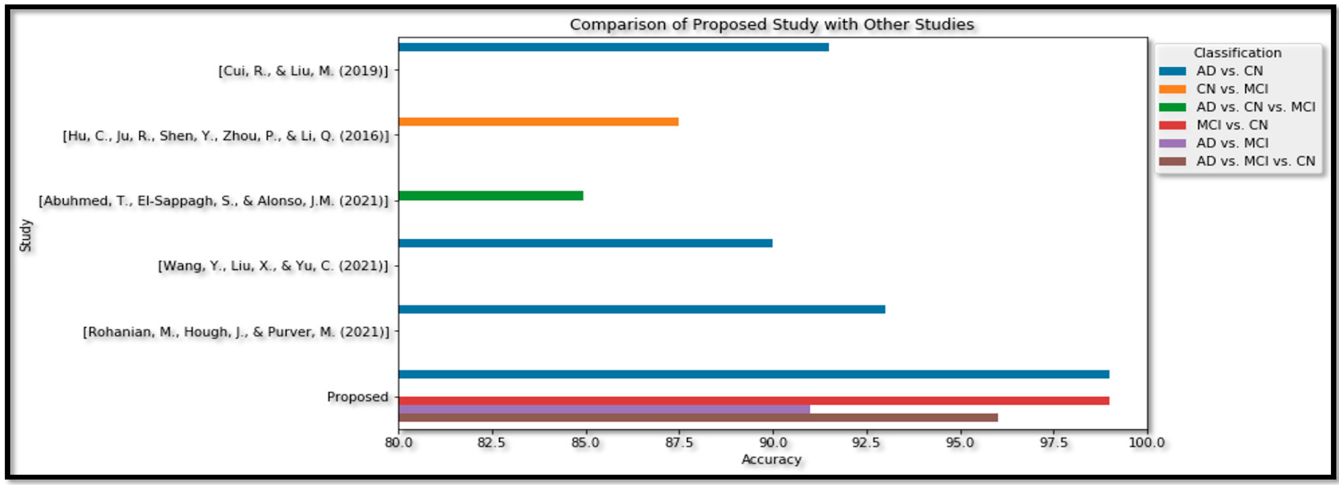
Table 7. Exiting proposed method comparison with the other method in the multimodality.

S. No	Author	Data Base	Method	Binary Class	Multi Class
1	[53]	ADNI	3D-CNN	AD vs. CN = 91.5	NA
2	[54]	ADNI	Soft Max Classifier	CN vs. MCI = 87.50	NA
3	[55]	ADNI	BiLSTM	NA	AD vs. CN vs. MCI = 84.95
4	[56]	ADNI	Feature Fusion	AD vs. CN = 90	NA
5	[57]	ADNI	Graph Fusion	AD vs. CN = 93	NA
6	Proposed	ADNI	Image Fusion + Feature-Level Fusion + Ensemble method	AD vs. CN = 99 MCI vs. CN = 99 AD vs. MCI = 91	AD vs. MCI vs. CN = 96

.

The proposed study, as shown in the table, utilized a combination of image fusion, feature-level fusion, and ensemble methods for classification. For the Binary classification of AD vs. CN, an accuracy of 99% was achieved, which is higher than the accuracies obtained in other studies. In the Binary type of MCI vs. CN, an accuracy of 99% was obtained. For the Binary classification of AD vs. MCI, an accuracy of 91% was achieved.

For the Multi Class category of AD vs. MCI vs. CN, an accuracy of 96% was obtained. The author reports that this result outperforms the Multi Class classification accuracy of 84.95% [32]. Hence, from the above table, we can see that the proposed model shows an effective (A_cc) in terms of the Binary Class and Multi Class classification in Figure 19.

6. Conclusions

The prediction of AD and its stages is widely explored in this article using the multimodal approach. An automatic pipeline method called Free Surfer helps to combine two modalities (PET and MRI) through the affine registration method. This whole technique uses pixel-level fusion. Then, these fused and non-fused outcomes are again processed for feature extraction. The extracted features, including volume, area, curving, folding, standard deviation, and mean, are from different brain cortical and subcortical regions, including the Hp, amygdala, and putamen. The features are fused for both modalities, and unnecessary elements are removed, leaving only the optimum characteristics for classification. Techniques such as ANOVA, scalar, Random Forest classifier, and correlation are used to select the prominent features. Those features are passed through various ML trending methods, including LR, DT, RF, GB, AB, KNN, GNB, SVM, MLP, SVM-RBF, and EL. Specifically, the EL methods are SVM_RBF + AB + GB + RF and GB + SVM_RBF. In a Binary classification of AD vs. CN, most models achieved an adequate (A_cc) of 99%. For MCI vs. CN, high (A_cc) scores were found using SVM, RF, GB, and AB models; that is, 99%. The (A_cc) of AD to MCI detection was lower than other Binary classifications, but an ensemble model (SVM_RBF + AB + GB + RF) still achieved 91% (A_cc). For AD vs. MCI vs. CN analysis, the ensemble model (GB + SVM_RBF) had the highest (A_cc) score of 96%. Therefore, the image- and feature-level fusion techniques demonstrate potential as features for ensemble classification models, which perform sustainably in Binary and Multi Class classification. Our subsequent analysis in future work will focus on identifying which regions provide the most prominent features for detecting AD, MC, and CN.