Article

A Diabetes Prediction System Based on Incomplete Fused Data Sources

1
School of Computer Sciences and Technology, Harbin Institute of Technology, Weihai 264209, China
2
Department of Endocrinology and Metabolism, Weihai Municipal Hospital, Affiliated to Shandong University, Weihai 264209, China
3
CAS Key Laboratory of Bio-Medical Diagnostics, Suzhou Institute of Biomedical Engineering and Technology Chinese Academy of Sciences, Suzhou 215163, China
4
School of Information Science and Technology, Nantong University, Nantong 226019, China
*
Author to whom correspondence should be addressed.
These authors contributed equally to this work.
Mach. Learn. Knowl. Extr. 2023, 5(2), 384-399; https://doi.org/10.3390/make5020023
Submission received: 12 December 2022 / Revised: 9 February 2023 / Accepted: 2 March 2023 / Published: 10 April 2023

Abstract

:
In recent years, the diabetes population has grown younger. Therefore, it has become a key problem to make a timely and effective prediction of diabetes, especially given a single data source. Meanwhile, there are many data sources of diabetes patients collected around the world, and it is extremely important to integrate these heterogeneous data sources to accurately predict diabetes. For the different data sources used to predict diabetes, the predictors may be different. In other words, some special features exist only in certain data sources, which leads to the problem of missing values. Considering the uncertainty of the missing values within the fused dataset, multiple imputation and a method based on graph representation is used to impute the missing values within the fused dataset. The logistic regression model and stacking strategy are applied for diabetes training and prediction on the fused dataset. It is proved that the idea of combining heterogeneous datasets and imputing the missing values produced in the fusion process can effectively improve the performance of diabetes prediction. In addition, the proposed diabetes prediction method can be further extended to any scenarios where heterogeneous datasets with the same label types and different feature attributes exist.

1. Introduction

The prevalence of diabetes is rising all over the world. According to the statistics from the International Diabetes Federation (IDF), about 425 million adults worldwide were diagnosed with diabetes in 2017. Following this trend, it is estimated that by 2045, the number of diabetic patients in the world will exceed 629 million [1]. Diabetes is a major cause of blindness, kidney failure, heart attack, stroke and lower-limb amputation, bringing huge inconvenience to the patients and even being life-threatening in severe cases. If it can be detected early and intensive treatment be offered, about half of those diabetes patients can go into remission.
At present, machine learning is an important research direction due to its high efficiency, accuracy, and extraordinary learning speed, and it plays a huge role in many fields, such as computer vision [2], natural language processing [3,4], stock market analysis [5], etc. In the 1980s, machine learning was used to predict diabetes. In 1988, Smith [6] constructed an early neural network model to study diabetes prediction in Pima Indians. He compared and analyzed the results with Logistic Regression (LR) and Linear Perceptron (LP). In 2004, Meiland [7] established a model based on LR to predict the presence of asymptomatic bacteriuria in diabetic women according to clinical indicators such as medical history and white blood cell count. In 2011, Ahmad A [8] compared the performance of decision trees and neural networks in diabetes prediction. In 2013, Kumari [9] used the backpropagation algorithm to provide an effective method for the automated examination of diabetes. In 2017, Maniruzzaman et al. [10] proposed a Gaussian Process (GP)-based model for diabetic classification of existing techniques such as Naive Bayes (NB), Linear Discriminant Analysis (LDA) and Quadratic Discriminant Analysis (QDA). In 2018, Swapna and Vinaya Kumar [11] used a deep learning method for detecting diabetes. In their study, Long Short-Term Memory (LSTM), Convolutional Neural Network (CNN) and a combination thereof were adopted to obtain dynamic features and then pipelined to Support Vector Machine (SVM) for classification.
All these studies have improved the prediction performance of diabetes. However, they are only based on a single small dataset. Considering that a single dataset contains limited information and there are many diabetes datasets, an effective method to promote diabetes prediction performance should be combining the multiple heterogeneous datasets. It should be noted that the process of combining datasets is also a feature-fusion process. Different datasets contain different feature information, and the features contained in different datasets will be fused when combined with different datasets. For feature fusion, many datasets are multi-dimensional. For example, the characteristics of a flower can be shape, color, and so on. These characteristics determine which breed it belongs to. We can also infer its species by its smell, flowering period, and geographical distribution. Therefore, if we combine these characteristics together, then the prediction of the flower varieties should be more accurate. In fact, this process can be viewed as multi-view learning [12,13,14]. In the process of feature fusion, the common features of heterogeneous datasets are directly integrated. Some specific features will be missed during the fusion process. Thus, some missing-value handling methods are needed to solve this problem and form a complete dataset.
For missing value handling strategies, there are three categories of approaches to deal with missing values. The first category is to remove all samples with missing values [15]. This is simple and intuitive; it will encounter huge problems when a large number of data values are missing. Unlike the first category, the second category chooses to impute the missing values. There are many common imputation methods, including Mean Imputation [16], Random Imputation within Classes [17], Gaussian copula imputation [18], etc. Commonly used ones include Regression Imputation [19], Support Vector Machine Imputation (SVM) [20], Multiple Imputation (MI) [21], Genetic Algorithm [22], graph-based imputation [23], etc. These imputation methods can effectively impute the missing values, but the imputation effect is different. The third category uses the indicator matrix to indicate the position of the missing values in the dataset, ignoring the marked missing values in the subsequent training and prediction process, and only uses the non-missing parts [24,25]. The second category is the most commonly used one among these three categories, and multiple imputation is the most popular one among the methods based on imputation.
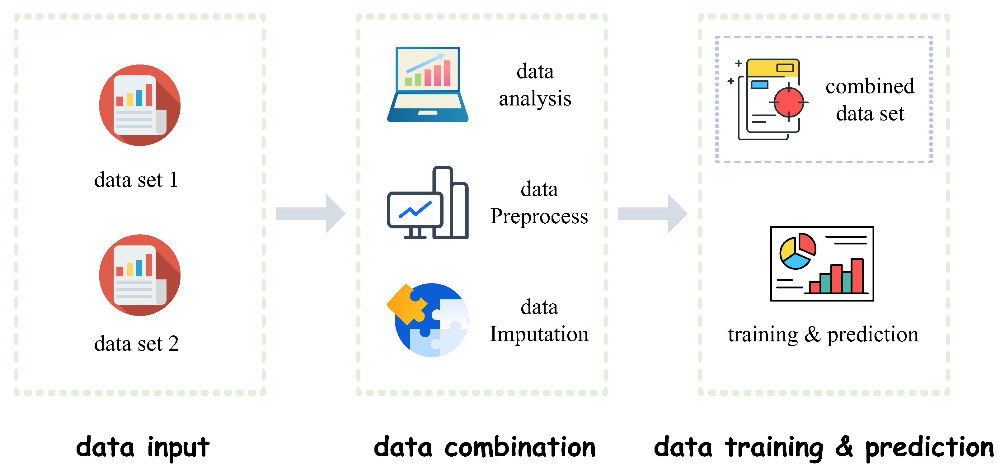
As for diabetes prediction, besides the most critical glycemic indicator, different hospitals or institutions will also consider other indicators to help them determine whether a patient has diabetes. These indicators may be differentiated and of different dimensions. In other words, there is heterogeneity between datasets. Since different indicators in the heterogeneous datasets all reflect some information related to diabetes, from the perspective of feature fusion, it is necessary to fuse them together. After fusion, the new dataset contains the characteristics of the original two datasets, which theoretically improves the prediction effect of diabetes. Therefore, in this paper, we will propose a new diabetes prediction system that can combine heterogeneous data sources. The system fused the common and special features within two data sources and missing values occurred during this process. For the missing value handling problem, we adopt multiple imputation and the graph representation learning model to impute the data to feed LR [26] to train and predict diabetes. To further improve the prediction results, we also introduce ensemble learning framework stacking [27,28], and finally further improve the prediction performance.
The main contributions of this paper are summarized as follows:
  • Explore and improve diabetes prediction by fusing two heterogeneous datasets from different sources, which can be generalized to more than two data sources and different application domains.
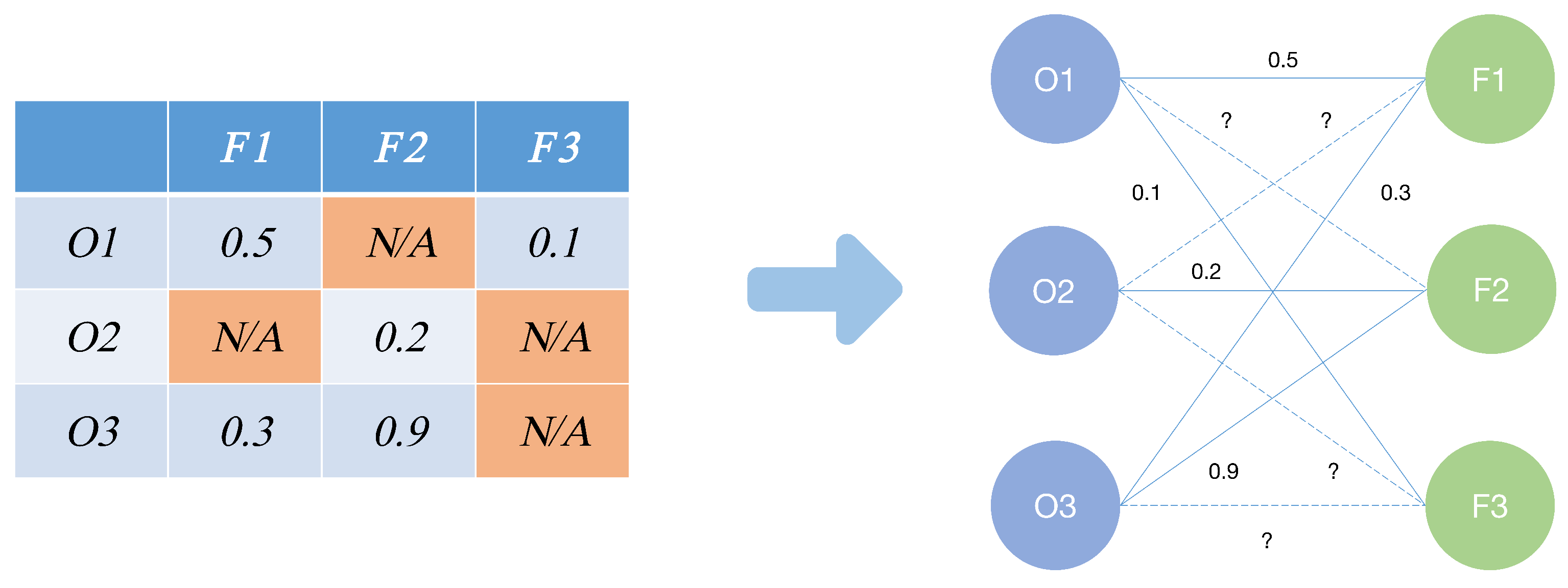
  • Taking the uncertainty of the missing values into consideration, graph representation learning is adopted to impute the missing values within the fused dataset.
  • Compared with the prediction results of the original dataset, the prediction results of the fused dataset are improved, and the stacking strategy further improves the performance.
The rest of this paper is organized as follows: Section 2 elaborates the overall framework of the system, introducing the specific functions of each module. Section 3 demonstrates the experiments, including dataset description, experimental settings, experimental evaluation metrics, experimental results and the analysis. In Section 4, we discuss the experimental results. Finally, Section 5 concludes the paper.

2. Heterogeneous Data Source Combination System Framework

The system framework in Figure 1 demonstrates the main process to combine data sources and predict diabetes. The whole system consists of three stages: data input, data combination, data training and prediction. Two heterogeneous datasets are fed as input, a new fused dataset is obtained by data combination, and then training and prediction are carried out to output the prediction result of diabetes. The details of these three phases are described below.

2.1. Data Input

At this stage, we feed two different datasets to predict diabetes. The features of these two datasets can be divided into common parts and specific parts, and the labels of those samples, being positive or negative, are retained.

2.2. Data Combination

2.2.1. Data Analysis

In this section, for the two datasets, we first calculate the correlation between the features of the datasets and the labels, and then analyze which features have a greater impact on the prediction of diabetes. These features are supposed to be extracted as the features of the combined dataset. Essentially, this is the feature selection or feature reduction. In addition, some advanced machine learning methods, such as supervised nonnegative matrix factorization and attribute reduction [29,30,31], can also be adopted.

2.2.2. Data Preprocess

Before combination, the original datasets should be preprocessed to eliminate abnormal samples. For the few missing values in the datasets, we can choose to remove them directly, or we can use common imputation methods (such as mean imputation) to impute the missing values. In short, what we do is ensure that the input data are reasonable.

2.2.3. Data Imputation

After data preprocessing, there should be no missing data in the two original datasets. Then, we start to combine heterogeneous data sources. Let P = { p 1 , p 2 , , p s } be all the feature sets in the first dataset, and Q = { q 1 , q 2 , , q t } be all the feature sets in the second dataset. A i p ( i = 1 , 2 , , m ; p = p 1 , p 2 , , p s ) represents the p-th feature corresponding to the i-th sample in the first dataset, B j q ( j = 1 , 2 , , n ; q = q 1 , q 2 , , q t ) represents the q-th feature corresponding to the j-th sample in the second dataset. When combining data, let S = P Q be the feature sets shared by P and Q , and union the sample with the shared features in data A ( S ) and B ( S ) to obtain D 1 , i.e., D 1 = A ( S ) B ( S ) . Let R = P Q be the feature sets that exist in P but do not exist in Q , then set the sample in the second dataset B ( R ) = N a N , union the sample to obtain D 2 = A ( R ) B ( R ) . In the same way, let T = Q P , set the sample in the first data A ( T ) = N a N , and union the sample to obtain D 3 = A ( T ) B ( T ) . In the end, the final combined dataset is D = D 1 D 2 D 3 .
As long as there are different features in the two different datasets, there must be missing values in the new dataset. Next, two imputation models will be used to impute missing values.
1. Multiple Regression. The main idea of multiple regression imputation model is to fit multiple regression models to missing variables and complete data variables to predict missing values [32]. For each missing value, we regard the missing variable as the dependent variable and the related variable (other non-missing variables) as the independent variable, perform regression fitting, then use the predicted value as the imputed value. We repeat the above process to generate m datasets, integrate the datasets together, then evaluate the model, and finally output a complete dataset.
2. GRAPE. Traditional missing value imputation methods include simple mean imputation and median imputation, etc., and complex ones such as k-neighbor imputation, regression imputation and so on [33]. However, some imputation methods based on deep learning, such as graph representation learning, are rarely considered to impute missing values. GRAPE is a graph-based representation learning method, which has good performance in feature imputation and label prediction [23]. In the GRAPE framework, feature imputation is transformed into an edge-level prediction task and label prediction into a node-level prediction task according to the bipartite graph model. These tasks are then solved using graph neural networks. The main steps are as follows:

Transform the Dataset into a Graph Structure

The main idea of the GRAPE model is to represent the missing dataset as a bipartite graph. In Figure 2, F j ( j = 1 , 2 , 3 ) represents the jth feature of the sample, O i ( i = 1 , 2 , 3 ) represents the ith sample, R ( O i , F j ) represents the value corresponding to the jth feature of the ith sample. For example, R ( O 1 , F 1 ) = 0.5 . Taking O 1 , O 2 , , O i as the nodes on one side of the bipartite graph, and F 1 , F 2 , , F j as the nodes on the other side of the bipartite graph, the nodes on both sides correspond to the edges formed by the connection, which is R ( O , F ) . R ( O , F ) is the feature value of the corresponding sample. If the feature of the sample is missing, the corresponding connection is missing. The nodes of the bipartite graph are represented in the form of one-shot vectors, which is convenient for subsequent input.

Use a Trained GNN (Graph Neural Network) to Calculate the Embedding of Each Vertex and Corresponding Known Edge

The embedding of an element is the vector calculated by propagating the element to the hidden layer. Based on a trained GNN, each element can be transmitted to the hidden layer from its own one-shot representation, and then extract the hidden layer vector as its own embedding [34]. An embedding can be regarded as a new feature vector, which contains information between elements. These embeddings are used as the input of the imputation model to impute missing values.

Use of MLP (Multilayer Perceptron) Model for Data Imputation

The nodes on one side of the bipartite graph are used as the input layer of the MLP, and the nodes on the other side are used as the output layer. Here, the MLP can in fact be viewed as a GNN over a complete graph, where the message function is matrix multiplication. GRAPE extends a simple MLP by allowing it to operate on sparse graphs, enabling it for missing feature imputation tasks by adopting a more complex message computation. For more detail, refer to GRAPE [23].
Through data analysis, data preprocessing and data imputation, a fused complete dataset can be finally obtained. This dataset contains the features extracted from the original two datasets, and each sample has a corresponding feature value. Then we use this dataset for training and prediction.

2.3. Data Training and Prediction

In this step, we use the basic model and the stacking method of ensemble learning [35] to train and make prediction. The main idea of the stacking method in the ensemble learning paradigm is as follows. First, the dataset is evenly divided into k parts, any one part is used as the test data, and the remaining k 1 parts are used as training data. The k basic models are employed to train and predict the data, and then the predicted results are combined to form a single dataset. Finally, a meta-model is used to train this dataset and obtain the final result. We chose five basic models (decision tree, random forest, LDA (linear discriminant analysis), KNN, Naive Bayes) and a meta-model (LR) for training and prediction. Its algorithm is shown in Algorithm 1.
Algorithm 1 Algorithm of Stacking
Require: Training Set D = { ( x 1 , y 1 ) , ( x 2 , y 2 ) , , ( x m , y m ) } ;
     Basic Model b 1 , b 2 , , b T ;
     Meta-Model m
1:
for  t = 1 T  do
2:
       h t = b t ( D ) ;
3:
end for
4:
D = ;
5:
for  i = 1 m  do
6:
      for  t = 1 T  do
7:
          z i t = h t ( x i ) ;
8:
      end for
9:
       D = D ( ( z i 1 , z i 2 , , z i T ) , y i ) ;
10:
end for
11:
h = m ( D ) ;
Ensure: H ( x ) = h ( h 1 ( x ) , h 2 ( x ) , , h T ( x ) )
The fused dataset is divided into training and test sets, and then the above models are used for training to predict, respectively, the samples belonging to the first data source in the test set, the samples belonging to the second data source, and all the samples in the test set to obtain the results.

3. Experiment

3.1. Dataset Description

There are two datasets used in this experiment, namely the Weihai Municipal Hospital(WMH) Diabetes Dataset and the Pima Indian Diabetes Dataset. The WMH dataset comes from a municipal hospital in Weihai City, Shandong Province, China. It records 12 diabetes-related diagnostic indicators of 118 local patients in Weihai, including gender, age, BMI, family history, insulin, blood sugar, serum C-peptide, and so on. The Pima dataset contains diabetes indicators including Pregnancies, Glucose, Insulin, Blood Pressure, Skin Thickness, Diabetes Pedigree Function, BMI, etc. of 768 Pima Indian women with potential diabetes from Phoenix, Arizona [36]. Both datasets contain the diagnosis labels of each patient (ill or not). According to the advice from doctors and some conclusions from previous research [37], six important features (gender, age, BMI, blood glucose, proinsulin and Cp120) are selected from the former dataset and five features (gender, age, BMI, blood glucose and diabetes pedigree) from the latter one to form seven common features. The features shared by the two datasets include gender, age, BMI, and blood glucose. Table 1 is a detailed description of the features.

3.2. Experimental Settings

After the dataset fusion process, we selected the multiple imputation and the GRAPE model to fill in the datasets, and obtained two complete fused datasets. The LR model and the stacking model in the ensemble learning framework are selected to train and predict whether the person is diabetic. Five basic models—random forest, decision tree, LDA, KNN, and Naive Bayes—and a meta-model LR are adopted in the stacking model. To verify the effectiveness of the proposed methods, five performance evaluation metrics—accuracy, precision, recall, F1-score, AUC (Area Under Curve)—are used in our experiments, and five-fold cross-validation is adopted to run the experiments. The average results and standard deviations are reported. Cross-validation can decrease the impact brought about by the different distributions of training data and test data.
Experiment 1. Use the LR model to train and predict on the original dataset.
Experiment 2. Use the multiple imputation model and GRAPE model for data imputation on the fused dataset, and use LR model and stacking model for training and prediction. Train the models on the training set containing both WMH and Pima samples, and then predict the WMH samples and Pima samples in the test set, respectively.
Experiment 3. Use the multiple imputation model and GRAPE model for data imputation on the fused dataset, and use LR model and stacking model for training and prediction. Split the fused dataset into the WMH samples and Pima samples, and then train and predict on WMH samples and Pima samples, respectively.
Experiment 4. Compare the methods “Complete GRAPE” and “GRAPE”. When the GRAPE model is used to impute the missing values, in fact, it will impute all the values including the existing values and the missing values. When we adopt LR to do the training, and use the complete data obtained after GRAPE, we call this method “Complete GRAPE”. If the dataset keeps the existing values and just replaces missing values with the imputed values obtained from GRAPE, we call the method employed on this dataset “GRAPE”. We will use them to predict the labels of WMH samples, Pima samples, and all samples in the test set.
Experiment 5. Compare the methods “LR+GRAPE” and “GRAPE”. For the basic model LR, the data after GRAPE imputation is divided into training and test sets, LR is trained on the training set and prediction is performed on the test set. This method is named “LR+GRAPE”. It is noted that GRAPE can predict the label in the test set without the help of any additional classification model. In Figure 2, running GRAPE with the label as node, the label corresponding to each sample in the test set will be given. This method is named “GRAPE”. We will use them to predict the labels of WMH samples, Pima samples, and all samples in the test set.
Since we use five-fold CV, all the above experiments are run five times, and the mean and standard deviation of the five results are taken as the final result.

3.3. Evaluation Metrics

Five evaluation metrics—accuracy, precision, recall, F1-score, and AUC (Area Under Curve)—are adopted in the experimental comparison. Since the first four are based on the confusion matrix, we will introduce the confusion matrix first. 
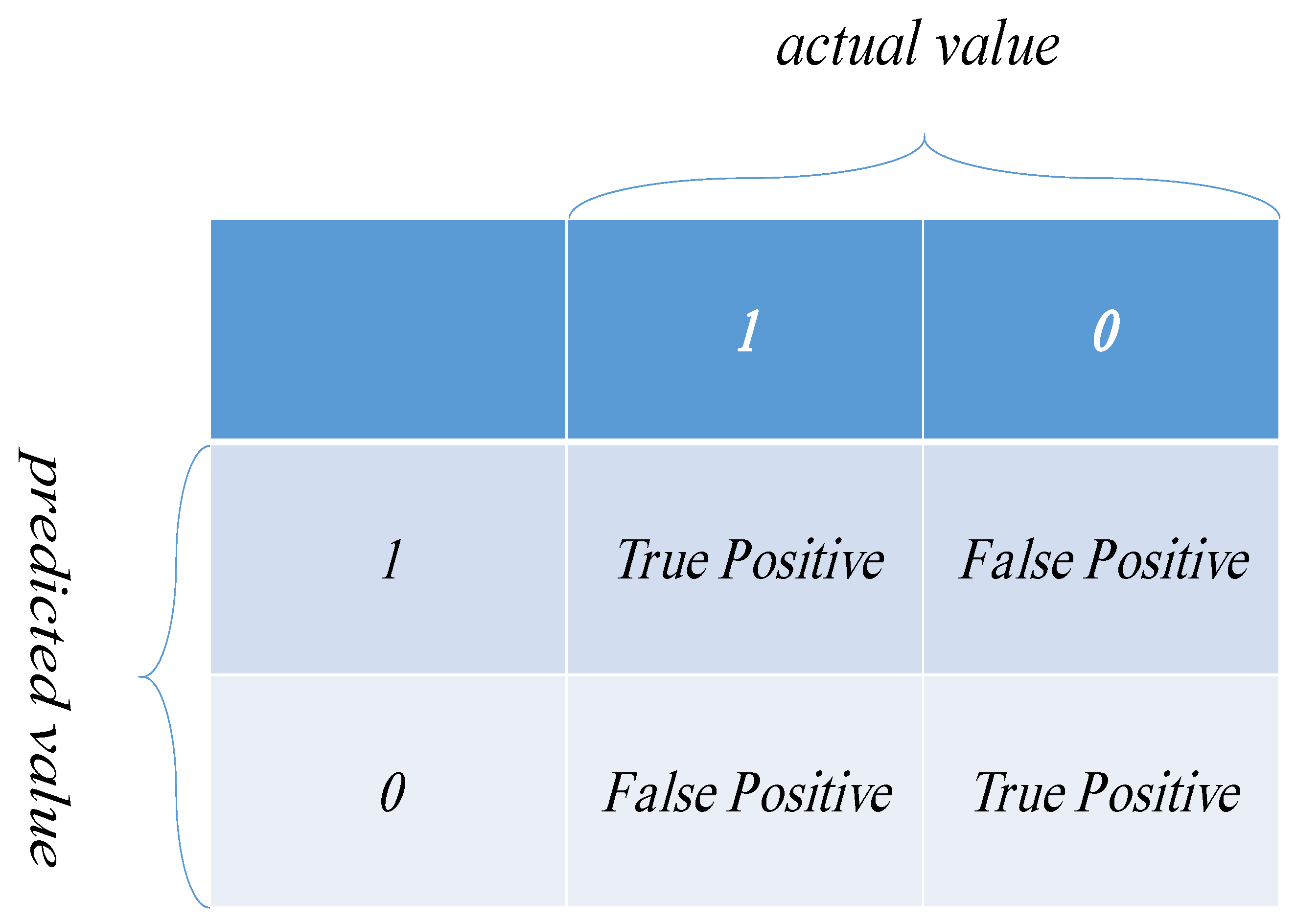
Figure 3 is the structure of the confusion matrix. The confusion matrix is a two-dimensional matrix, which is mainly used to evaluate binary classification problems and reflect the difference between the predicted result and the actual result [38]. It can be seen from the matrix that there are two types of category (0 and 1), and the difference between the category predicted by the model and the true categories forms four indicators, respectively. They are true positive (TP), false positive (FP), false negative (FN) and true negative (TN). TP represents the number of samples whose predicted result is 1 and the true result is 1, and FP represents the number of samples whose predicted result is 1 but the actual result is 0. TN represents the number of samples whose predicted result is 0 and the true result is 0, and FN represents the number of samples whose predicted result is 0 but the actual result is 1.
The calculation formula for accuracy is
A c c u r a c y = T P + T N T P + T N + F P + F N
It reflects the proportion of the correctly predicted sample to the total sample.
The calculation formula of precision is
P r e c i s i o n = T P T P + F P .
It reflects the accuracy of the positive class and measures the correctness of the prediction of the positive class.
The calculation formula of recall is
R e c a l l = T P T P + F N .
It indicates how many samples with positive labels are predicted correctly.
Precision and recall are often relative. Sometimes precision is high but recall is low, so F1-score is introduced to provide a trade-off. F1-score is an evaluation index that combines precision and recall. Its calculation formula is
F 1 = 2 T P 2 T P + F N + F P
It is the harmonic mean of precision and recall.
The last one, AUC, refers to the area between the ROC (Receiver Operating Characteristic) curve and the x-axis. It can quantitatively display the classification of the model. Generally, the larger the value of AUC, the better the classification performance on the dataset.
In the context of medicine, especially in clinical decision support, the AUC is often too general in that it assesses all decision thresholds, including unrealistic ones. Conversely, accuracy, precision, recall, positive predictive value, and the F1 score are too specific; they are measured against a single threshold that is optimal for some cases but not for others, which is not fair. Thus, each measure has its limit, all of them will be adopted to evaluate the result. A very recent work [39] describes a deep ROC analysis to measure performance in multiple groups of predicted risk or in groups of TP rate or FP rate. It is interesting that these authors also provide a Python toolkit.

3.4. Experimental Results

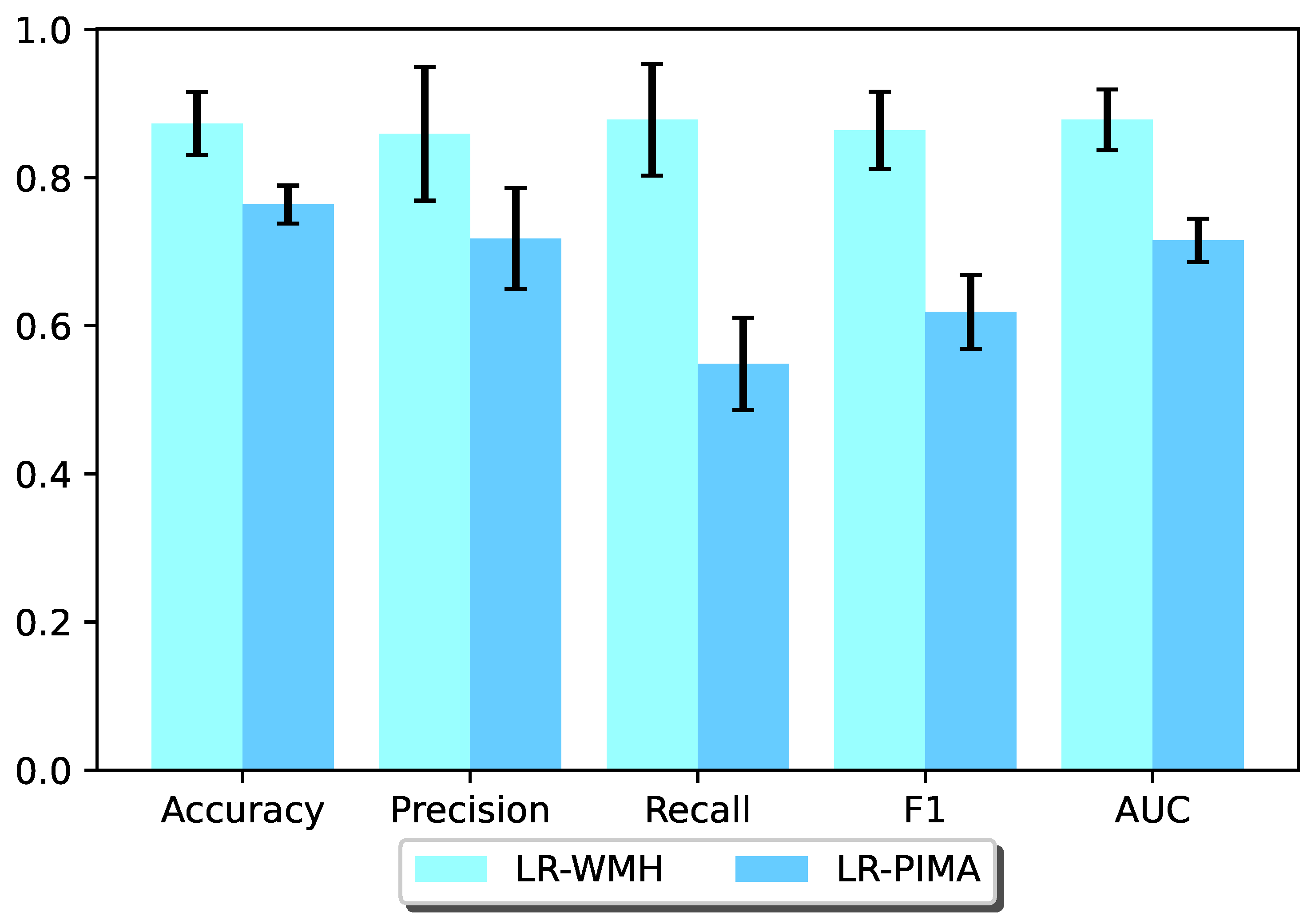
The results of Experiment 1 and Experiment 2 are shown in Figure 4, Table 2 and Table 3. From Table 2, we can find that both the MICE filling model and the GRAPE imputation model have improved the prediction results of WMH samples slightly, and the performance obtained using the stacking model is better than that obtained by the LR model. Regarding the WMH data, it achieves the best performance with an accuracy of 92.5% using the GRAPE model for data imputation and the stacking model for training and prediction. From Table 3, it can be seen that compared to the WMH dataset, Pima’s prediction results are slightly improved. On the whole, for Pima dataset, it can be improved slightly using the MICE filling model to impute and using the stacking model to predict.
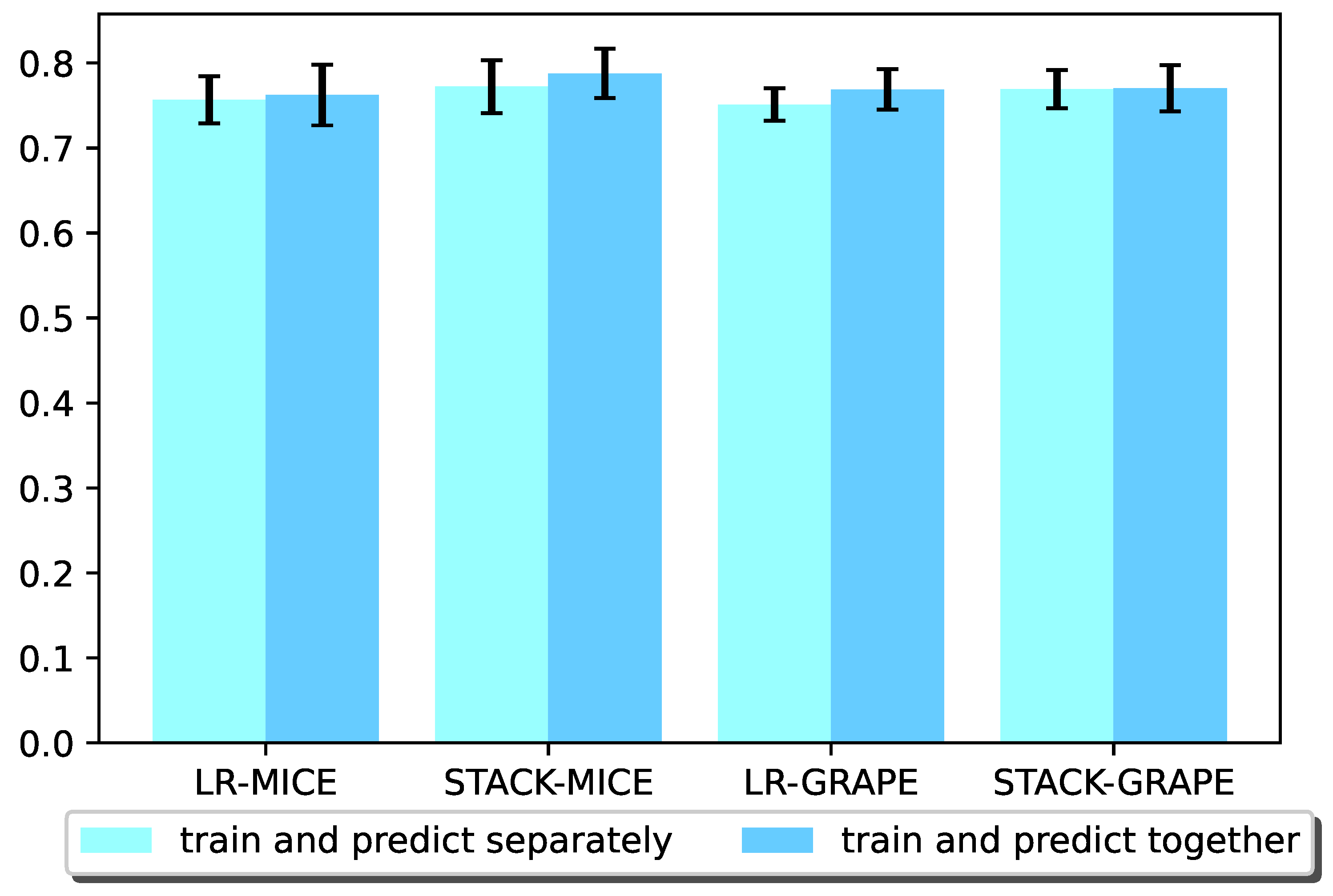
For Experiment 3, Figure 5 shows the result comparison of training on fused training samples to predict Pima test samples and separate training on Pima training samples and then predicting Pima test samples. 
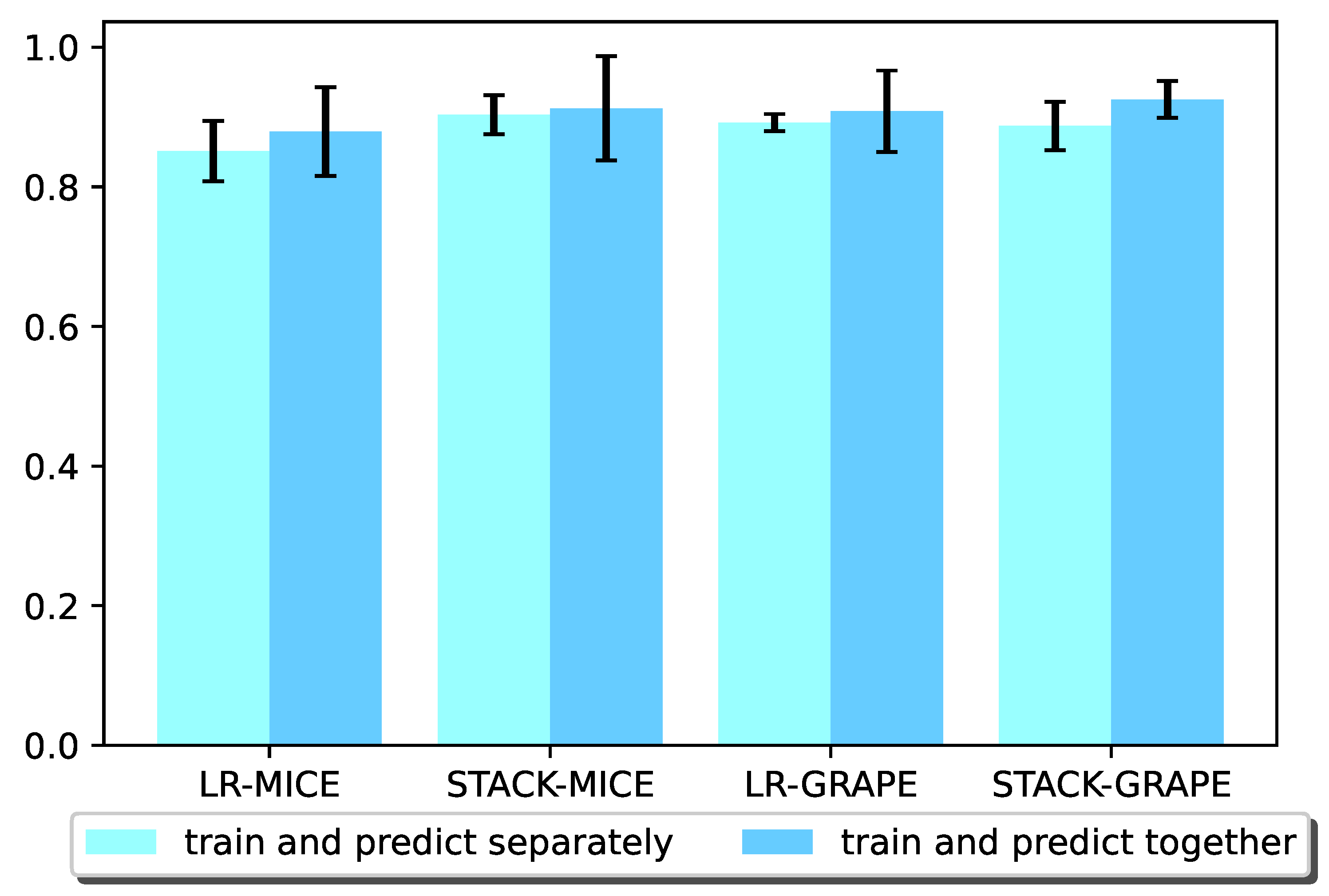
Figure 6 shows the result comparison of training on fused training samples to predict WMH test samples and separately training on WMH samples and then predicting WMH test samples. It can be seen from the results that for both Pima samples and WMH samples, the results of separate training and prediction are generally not as good as those results obtained with training and predicting together.
For Experiment 4, Table 4 and Table 5 demonstrate the results of the two methods “GRAPE” and “Complete GRAPE”. From these two tables, we can see that it is slightly better to use the imputed dataset obtained from “Complete GRAPE” for WMH dataset than that obtained from “GRAPE” in recall, but slightly worse in precision, F1-score and AUC. For Pima data, it seems that “Complete GRAPE” performs worse than “GRAPE” in most of the evaluation metrics. On all data, “Complete GRAPE” performs slightly better than or as well as “GRAPE”. In summary, it seems that “Complete GRAPE” performs as well as “GRAPE”. This is indeed reasonable, because the imputed result of the GRAPE model for the position that already exists is very close to the actual value. It indicates that this has little influence on the prediction effect.
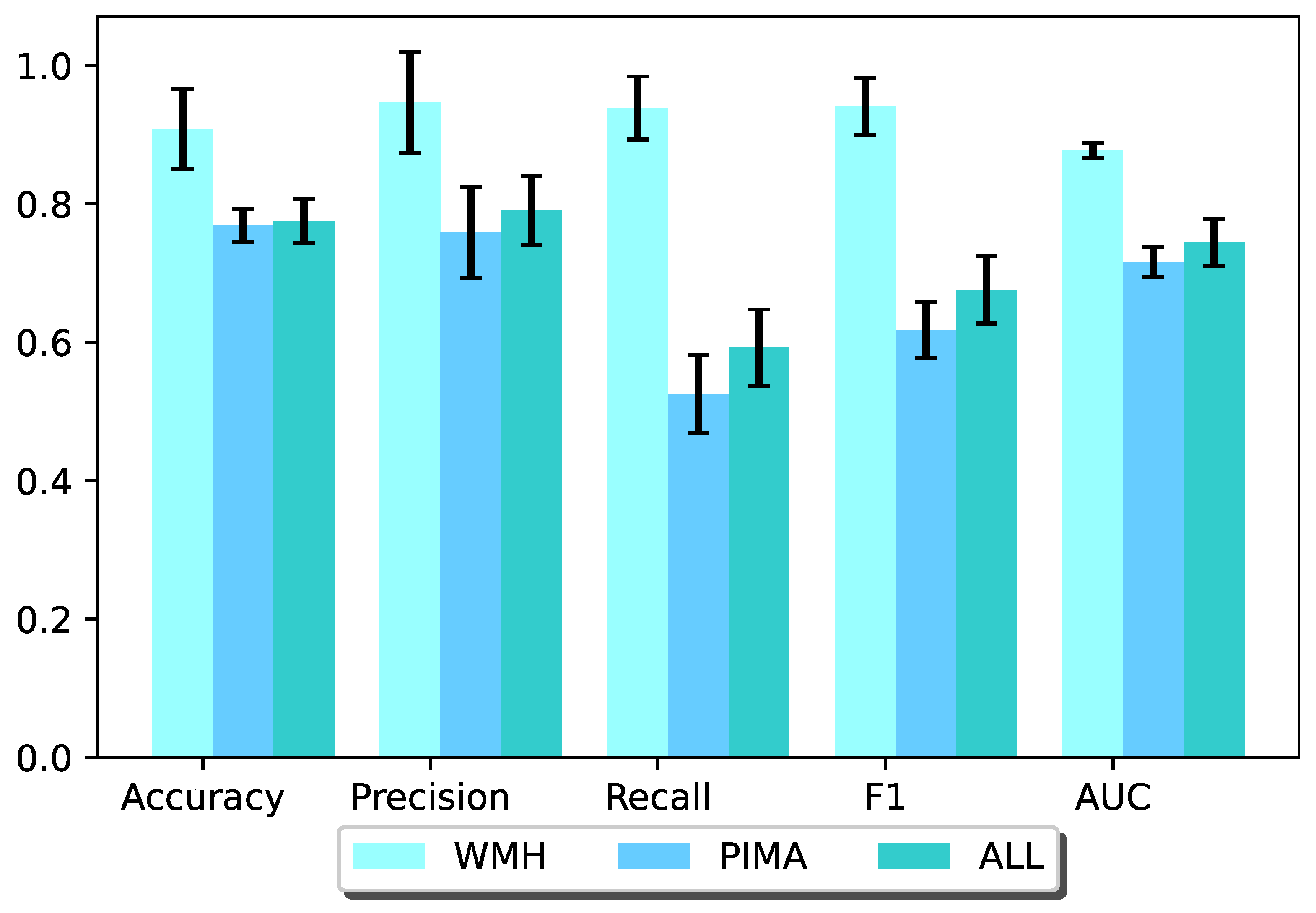
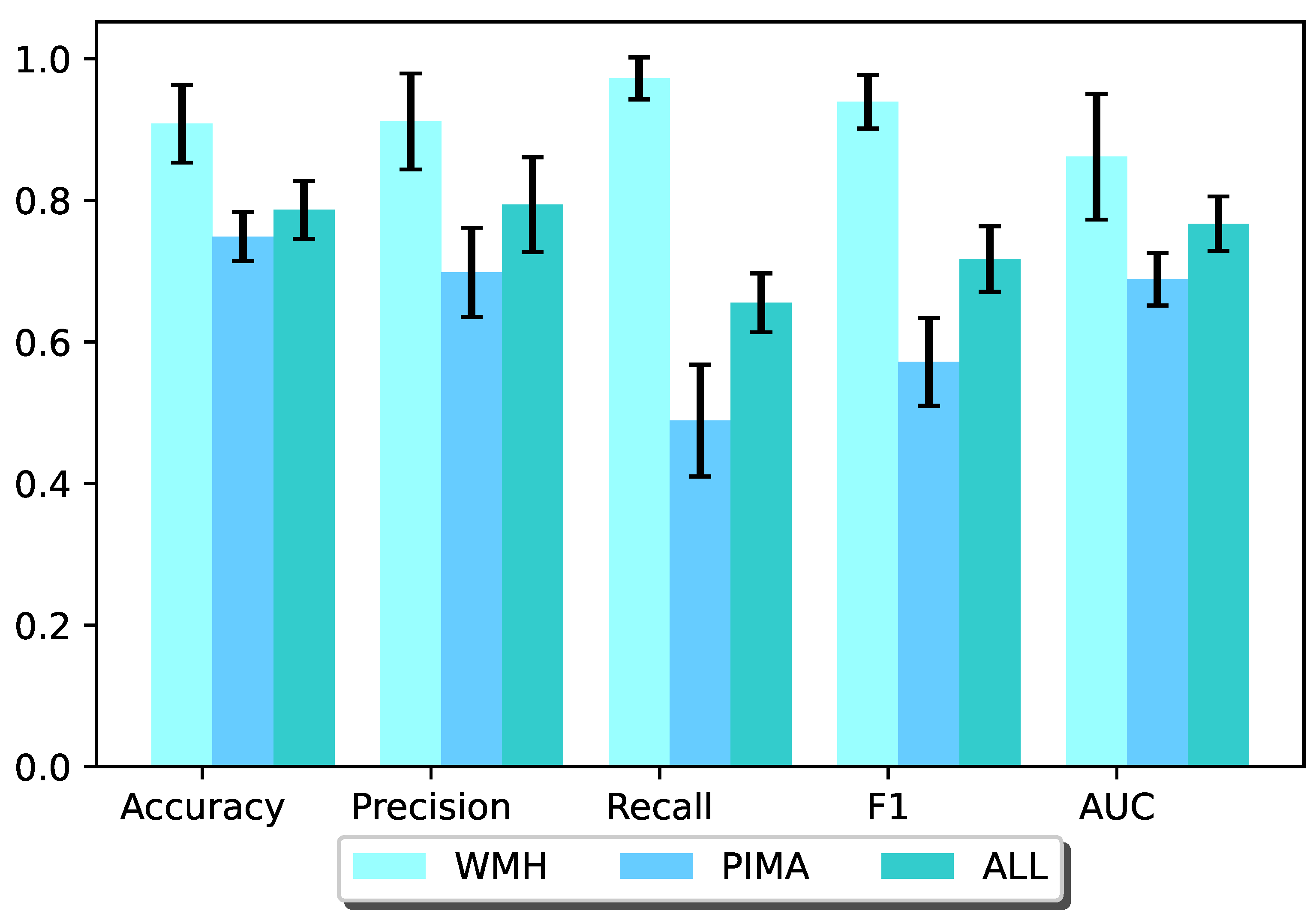
For Experiment 5, Figure 7 and Figure 8 show the predicted results of the two methods “GRAPE” and “LR+GRAPE”. From the results, we can find that the prediction results obtained from “GRAPE” are slightly better than or as well as that obtained from “LR+GRAPE”. Thus, it is better to directly use “GRAPE” to impute and predict than to run LR on the data after “GRAPE” imputation.
To see the boundary of the proposed method, we run the STACK-GRAPE on fused datasets with three missing ratios: 30%, 50% and 80%. For our fused dataset, its missing ratio is about 30%. We assume our fused dataset to be X with the size 986 × 7, to generate a dataset with missing ratios 50% and 80%, 20% and 50% of 6902 (986 × 7) entries are randomly removed from those observed positions. STACK-GRAPE is then run on these generated datasets. The results are shown in Table 6. From this result, we can see that the performance of STACK-GRAPE decreases when missing ratios increase, but even in the missing ratio 80%, the accuracy is still 0.676. Thus, this method applies to the high missing ratio.
Since ensemble learning framework stacking is used to predict diabetes, to understand the stacking model better, additional experiments with each sub-model are conducted and the results are shown in Table 7. From the results, we can find that Naive Bayes performs the worst, and random forest performs the best among the sub-models. The ensemble model STACK-GRAPE outperforms all the sub-models in the average cases.

4. Discussion

From the above experiments, it can be seen that the imputation model and the classifier adopted have an impact on the prediction performance of the fused datasets. As for the filling model, the more basic filling models such as mean filling and KNN filling are not suitable for multiple regression imputation. The deep-learning imputation model GRAPE seems the best option to impute the missing values in the fused dataset. GRAPE, a deep-learning imputation model, can act as a classifier besides the imputation model, and it performs well. In addition, the ensemble learning model stacking can boost the performance further, and some previous works [40,41] also verified this conclusion. However, these works cannot deal with missing-value problems, thus comparison cannot be done on prediction on incomplete datasets. In the process of fusing heterogeneous datasets, it is important to choose a suitable filling model. The better the filling model used, the more effective the information contained in the fusion dataset. With such a dataset, coupled with a good prediction model, the final prediction result will be satisfactory.
For the imputation model, besides multiple imputation and GRAPE, several other models are proposed to deal with missing values, such as LSTM [42]. Due to the introduction of a gating mechanism, LSTM is outstanding in the processing of the missing values of time-series problems. Compared with LSTM, GRAPE can deal with any missing case in any data. The idea of combining heterogeneous datasets and imputing the missing values incurred in the combining process is not only applicable to the problem of diabetes prediction, but also to all the disease prediction problems [43], even those outside the medical field. It is also interesting to consider missing-value imputation and diabetes prediction as multitask learning [44].
Although the proposed methods show their effectiveness, there is a limit for them. If the different data sources do not have common features, the proposed method cannot be directly uses. However, in real-world applications, different data sources collected with the same goal normally have some features in common, as well as some special features. Thus, when combining, it is better to make full use of their complementary and consensus information. It can be seen as multi-view learning [45,46] or multi-source learning. Thus, the tools used in those related areas can be borrowed to serve the current goal. In addition, we fused two data sources in this work, and in fact it is easy to extend to more than two data sources.

5. Conclusions

The prediction performance of this system obtained by combining two heterogeneous diabetes data sources and selecting an appropriate imputation model is better than those obtained on the original datasets. For the WMH dataset, the GRAPE model for imputation and the stacking model for training is the best combination. For the Pima dataset, the MICE model and the stacking model have the best prediction performance. This shows that the idea of combining heterogeneous datasets and imputing the missing values produced in the fusion process is effective to improve diabetes prediction performance. In fact, almost every hospital collected the heterogeneous diabetes datasets and they have not been exploited to serve for diabetes prediction. This paper provided a feasible and effective way to deal with this problem and shows great potential. Moreover, this idea may not only be used in diabetes prediction, but also can apply to any scenarios where heterogeneous datasets with the same label types and different feature attributes exist. In the current work, we did not investigate the impact caused by the different distribution of training data and test data. However, this fact indeed has an impact on the prediction performance. In future work, further research will be conducted.

Author Contributions

Conceptualization, Z.Y. and G.C.; methodology, H.D. and G.C.; software, H.D.; validation, Z.Y. and G.C.; formal analysis, G.C.; investigation, H.D.; resources, M.S.; data curation, M.S.; writing—original draft preparation, H.D. and Z.Y.; writing—review and editing, M.S., W.D. and L.W.; visualization, Z.Y.; supervision, G.C.; project administration, D.C. funding acquisition, G.C. All authors have read and agreed to the published version of the manuscript.

Funding

This work is supported by Young Teacher Development Fund of Harbin Institute of Technology IDGA10002071 and Key Research and Development Plan of Shandong Province 2021SFGC0104.

Institutional Review Board Statement

The study was conducted in accordance with the Declaration of Helsinki, and approved by the Ethics Committee of Weihai Municipal Hospital.

Informed Consent Statement

Patient consent was waived due to research involving the analysis of existing data, where the data will be analyzed such that individual subjects cannot be identified.

Data Availability Statement

The datasets generated and analyzed in the current study are available from the corresponding author on reasonable request.

Acknowledgments

The authors would like to thank H. Chen for running some preliminary experiments.

Conflicts of Interest

The authors declare that they have no conflict of interest.

References

  1. Moore, J.; Csikar, J.; Kang, J.; Tugnait, A.; Campbell, F.; Clerehugh, V. Awareness, practices, training, and confidence of Paediatric Diabetes Care Teams in relation to periodontitis. Pediatr. Diabetes 2020, 21, 384–389. [Google Scholar] [CrossRef] [PubMed]
  2. Kang, Y.; Chao, G.; Hu, X.; Tu, Z.; Chu, D. Deep Learning for Fine-Grained Image Recognition: A Comprehensive Study. In Proceedings of the 2022 4th Asia Pacific Information Technology Conference, Virtual Event, 14–16 January 2022; pp. 31–39. [Google Scholar]
  3. Chao, G.; Sun, S. Applying a multitask feature sparsity method for the classification of semantic relations between nominals. In Proceedings of the Machine Learning and Cybernetics (ICMLC), Xi’an, China, 15–17 July 2012; Volume 1, pp. 72–76. [Google Scholar]
  4. Zhang, B.; Tu, Z.; Jiang, Y.; He, S.; Chao, G.; Chu, D.; He, X. DGPF: A Dialogue Goal Planning Framework for Cognitive Service Conversation Bot. In Proceedings of the 2021 IEEE International Conference on Web Services, Chicago, IL, USA, 5–10 September 2021; pp. 335–340. [Google Scholar]
  5. Wang, Z.; Sun, Q.; Chao, G.; Cai, B.; Huang, Y.; Fu, Y. A Multi-view Time Series Model for Share Turnover Prediction. Appl. Intell. 2022, 52, 14595–14606. [Google Scholar] [CrossRef]
  6. Smith, J.W.; Everhart, J.E.; Dickson, W.; Knowler, W.C.; Johannes, R.S. Using the ADAP learning algorithm to forecast the onset of diabetes mellitus. In Proceedings of the Annual Symposium on Computer Application in Medical Care, Washington, DC, USA, 6–9 November 1988; p. 261. [Google Scholar]
  7. Meiland, R.; Geerlings, S.E.; Stolk, R.P.; Hoepelman, H. History taking and leukocyturia predict the presence of asymptomatic bacteriuria in women with diabetes mellitus. Eur. J. Epidemiol. 2004, 19, 1021–1027. [Google Scholar] [CrossRef] [PubMed]
  8. Ahmad, A.; Mustapha, A.; Zahadi, E.D.; Masah, N.; Yahaya, N.Y. Comparison between Neural Networks against Decision Tree in Improving Prediction Accuracy for Diabetes Mellitus. Commun. Comput. Inf. Ence 2011, 188, 537–545. [Google Scholar]
  9. Kumari, S.; Singh, A. A data mining approach for the diagnosis of diabetes mellitus. In Proceedings of the 7th International Conference on Intelligent Systems and Control, Coimbatore, India, 4–5 January 2013. [Google Scholar]
  10. Maniruzzaman, M.; Kumar, N.; Menhazul Abedin, M.; Shaykhul Islam, M.; Suri, H.S.; El-Baz, A.S.; Suri, J.S. Comparative approaches for classification of diabetes mellitus data: Machine learning paradigm. Comput. Methods Programs Biomed. 2017, 152, 23–34. [Google Scholar] [CrossRef]
  11. Swapna, G.; Kp, S.; Vinayakumar, R. Automated detection of diabetes using CNN and CNN-LSTM network and heart rate signals. Procedia Comput. Sci. 2018, 132, 1253–1262. [Google Scholar]
  12. Sun, S.; Chao, G. Alternative multi-view maximum entropy discrimination. IEEE Trans. Neural Netw. Learn. Syst. 2016, 27, 1445–1556. [Google Scholar]
  13. Ding, W.; Abdel-Basset, M.; Hawash, H.; Pedrycz, W. Multimodal Infant Brain Segmentation by Fuzzy-informed Deep Learning. IEEE Trans. Fuzzy Syst. 2021, 30, 1088–1101. [Google Scholar] [CrossRef]
  14. Chao, G.; Sun, S. Consensus and complementarity based maximum entropy discrimination for multi-view classification. Inf. Sci. 2016, 367, 296–310. [Google Scholar] [CrossRef]
  15. Chhabra, G.; Vashisht, V.; Ranjan, J. A Review on Missing Data Value Estimation Using Imputation Algorithm. J. Adv. Res. Dyn. Control. Syst. 2019, 11, 312–318. [Google Scholar]
  16. Yin, B.C.; Ng, D.G.Y. Response and Non-Response to a Quality-of-Life Question on Sexual Life: A Case Study of the Simple Mean Imputation Method. Qual. Life Res. 2006, 15, 1493–1501. [Google Scholar]
  17. Kalton, G. Compensating for Missing Survey Data; Survey Research Center, Insitute for Social Research: Ann Arbor, MI, USA, 1983. [Google Scholar]
  18. Zhao, Y.; Udell, M. Missing value imputation for mixed data via gaussian copula. In Proceedings of the 26th ACM SIGKDD International Conference on Knowledge Discovery & Data Mining, Virtual Event, 6–10 July 2020; pp. 636–646. [Google Scholar]
  19. Templ, M.; Kowarik, A.; Filzmoser, P. Iterative stepwise regression imputation using standard and robust methods. Comput. Stat. Data Anal. 2011, 55, 2793–2806. [Google Scholar] [CrossRef]
  20. Wang, L.H.; Gao, S.; Xing, Q.U. SVM Based Missing Data Imputation Algorithm in Nuclear Power Plant’s Environmental Radiation Monitor Sensor Network. J. Univ. South China 2012, 4, 14–17. [Google Scholar]
  21. Schafer, J.L. Multiple Imputation: A Primer. Stat. Methods Med. Res. 1999, 8, 3–15. [Google Scholar] [CrossRef] [PubMed]
  22. Tang, J.; Zhang, G.; Wang, Y.; Hua, W.; Fang, L. A hybrid approach to integrate fuzzy C-means based imputation method with genetic algorithm for missing traffic volume data estimation. Transp. Res. Part C 2015, 51, 29–40. [Google Scholar] [CrossRef]
  23. You, J.; Ma, X.; Ding, Y.; Kochenderfer, M.J.; Leskovec, J. Handling missing data with graph representation learning. Adv. Neural Inf. Process. Syst. 2020, 33, 19075–19087. [Google Scholar]
  24. Shao, W.; He, L.; Yu, P.S. Multiple incomplete views clustering via weighted nonnegative matrix factorization with regularization. In Proceedings of the Machine Learning and Knowledge Discovery in Databases: European Conference, ECML PKDD 2015, Porto, Portugal, 7–11 September 2015; Proceedings, Part I. Springer: Berlin/Heidelberg, Germany, 2015; pp. 318–334. [Google Scholar]
  25. Chao, G.; Sun, J.; Lu, J.; Wang, A.-L.; Langleben, D.D.; Li, C.-S.; Bi, J. Multi-view cluster analysis with incomplete data to understand treatment effects. Inf. Sci. 2019, 494, 278–293. [Google Scholar] [CrossRef]
  26. Hosmer, D.W.; Stanley, L. Goodness of fit tests for the multiple logistic regression model. Commun. Statist Theor. Meth 1980, 9, 1043–1069. [Google Scholar] [CrossRef]
  27. Yy, A.; Long, W.B.; Ying, H.A.; Yan, W.A.; Lh, C.; Sn, A. Classification of Parkinson’s disease based on Multi-modal Features and Stacking Ensemble Learning. J. Neurosci. Methods 2020, 350, 109019. [Google Scholar]
  28. Chao, G.; Wang, S.; Yang, S.; Li, C.; Chu, D. Incomplete Multi-View Clustering by Multiple Imputation and Ensemble Clustering. Appl. Intell. 2022, 52, 14811–14821. [Google Scholar] [CrossRef]
  29. Ding, W.; Lin, C.T.; Cao, Z. Deep neuro-cognitive co-evolution for fuzzy attribute reduction by quantum leaping PSO with nearest-neighbor memeplexes. IEEE Trans. Cybern. 2019, 49, 2744–2757. [Google Scholar] [CrossRef] [PubMed]
  30. Chao, G.; Mao, C.; Wang, F.; Zhao, Y.; Luo, Y. Supervised nonnegative matrix factorization to predict ICU mortality risk. In Proceedings of the 2018 IEEE International Conference on Bioinformatics and Biomedicine, Madrid, Spain, 3–6 December 2018; pp. 1189–1194. [Google Scholar]
  31. Ding, W.; Lin, C.T.; Cao, Z. Shared Nearest-Neighbor Quantum Game-Based Attribute Reduction With Hierarchical Coevolutionary Spark and Its Application in Consistent Segmentation of Neonatal Cerebral Cortical Surfaces. IEEE Trans. Neural Netw. Learn. Syst. 2019, 30, 2013–2027. [Google Scholar] [CrossRef]
  32. Shah, A.D.; Ba Rtlett, J.W.; James, C.; Owen, N.; Harry, H. Comparison of Random Forest and Parametric Imputation Models for Imputing Missing Data Using MICE: A CALIBER Study. Am. J. Epidemiol. 2014, 179, 764–774. [Google Scholar] [CrossRef] [Green Version]
  33. Gan, X.; Liew, A.W.C.; Yan, H. Microarray missing data imputation based on a set theoretic framework and biological knowledge. Nucleic Acids Res. 2006, 34, 1608–1619. [Google Scholar] [CrossRef] [Green Version]
  34. Ahmed, N.K.; Rossi, R.A.; Zhou, R.; Lee, J.B.; Kong, X.; Willke, T.L.; Eldardiry, H. A framework for generalizing graph-based representation learning methods. arXiv 2017, arXiv:1709.04596. [Google Scholar]
  35. Chatzimparmpas, A.; Martins, R.M.; Kucher, K.; Kerren, A. StackGenVis: Alignment of data, algorithms, and models for stacking ensemble learning using performance metrics. IEEE Trans. Vis. Comput. Graph. 2020, 27, 1547–1557. [Google Scholar] [CrossRef]
  36. Rubin, D.B. Multiple Imputation in Sample Surveys: A Phenomenological Bayesian Approach to Nonresponse. In Proceedings of the Survey Research Methods Section of the American Statistical Association, San Diago, CA, USA, 14–17 August 1978; American Statistical Association: Alexandria, VA, USA, 1978; pp. 20–28. [Google Scholar]
  37. Rajput, M.R.; Khedgikar, S.S. Diabetes prediction and analysis using medical attributes: A Machine learning approach. J. Xi’An Univ. Archit. Technol. 2022, 14, 8–103. [Google Scholar]
  38. Landgrebe, T.C.; Duin, R.P. Efficient Multiclass ROC Approximation by Decomposition via Confusion Matrix Perturbation Analysis. IEEE Trans. Pattern Anal. Mach. Intell. 2008, 30, 810–822. [Google Scholar] [CrossRef] [Green Version]
  39. Carrington, A.M.; Manuel, D.G.; Fieguth, P.W.; Ramsay, T.; Osmani, V.; Wernly, B.; Bennett, C.; Hawken, S.; Magwood, O.; Sheikh, Y. Deep ROC analysis and AUC as balanced average accuracy, for improved classifier selection, audit and explanation. IEEE Trans. Pattern Anal. Mach. Intell. 2023, 45, 329–341. [Google Scholar] [CrossRef]
  40. Tan, Y.; Chen, H.; Zhang, J.; Tang, R.; Liu, P. Early risk prediction of diabetes based on GA-Stacking. Appl. Sci. 2022, 12, 632. [Google Scholar] [CrossRef]
  41. Wang, J.; Liu, C.; Li, L.; Li, W.; Yao, L.; Li, H.; Zhang, H. A stacking-based model for non-invasive detection of coronary heart disease. IEEE Access 2020, 8, 37124–37133. [Google Scholar] [CrossRef]
  42. Wu, X.; Wang, H.-Y.; Shi, P.; Sun, R.; Wang, X.; Luo, Z.; Zeng, F.; Lebowitz, M.S.; Lin, W.-Y.; Lu, J.-J. Long short-term memory model–a deep learning approach for medical data with irregularity in cancer predication with tumor markers. Comput. Biol. Med. 2022, 144, 105362. [Google Scholar] [CrossRef] [PubMed]
  43. Zhang, P.; Wang, Z.; Chao, G.; Huang, Y.; Yan, J. An Oriented Attention Model for Infectious Disease Cases Prediction. In Proceedings of the International Conference on Industrial, Engineering and Other Applications of Applied Intelligent Systems, Shanghai, China, 19–22 July 2022; pp. 124–139. [Google Scholar]
  44. Chao, G.; Sun, S. Semi-supervised multitask learning via self-training and maximum entropy discrimination. In Proceedings of the International Conference on Neural Information Processing, Doha, Qatar, 12–15 November 2012; Springer: Berlin/Heidelberg, Germany, 2012; pp. 340–347. [Google Scholar]
  45. Chao, G.; Sun, S. Multi-kernel maximum entropy discrimination for multi-view learning. Intell. Data Anal. 2016, 20, 481–493. [Google Scholar] [CrossRef] [Green Version]
  46. Chao, G.; Sun, S. Semi-Supervised Multi-View Maximum Entropy Discrimination with Expectation Laplacian Regularization. Inform. Fusion 2018, 45, 296–306. [Google Scholar] [CrossRef]
Figure 1. An overview of heterogeneous data source combination system framework.
Make 05 00023 g001
Figure 2. The process of transforming a dataset into a graph in “GRAPE”.
Make 05 00023 g002
Figure 3. Confusion Matrix.
Make 05 00023 g003
Figure 4. The prediction of the LR model on the two original datasets.
Make 05 00023 g004
Figure 5. Comparison of the prediction accuracy of training on all samples and training only on Pima samples.
Make 05 00023 g005
Figure 6. Comparison of the prediction accuracy of training on all samples and training only on WMH samples.
Make 05 00023 g006
Figure 7. Results obtained with the method “GRAPE”.
Make 05 00023 g007
Figure 8. Results obtained with the method “LR+GRAPE”.
Make 05 00023 g008
Table 1. Description of the features in the combined dataset.
FeatureValue TypeDescription
Gender0 or 1gender
AgeIntegerage
BMIFloatBody mass index
Blood GlucoseFloatHuman blood glucose concentration
ProinsulinFloatinitial proinsulin level, measured 120 min after taking glucose
Cp120Floatinitial C−peptide level, measured 120 min after taking glucose
Diabetes PedigreeFloatcoefficient calculated by family members diabetes conditions
Table 2. Prediction results of WMH samples on the combined data set.
DatasetAccuracyPrecisionRecallF1-ScoreAUC
LR-WMH origin0.873 ± 0.0420.859 ± 0.0900.878 ± 0.0750.863 ± 0.0520.878 ± 0.041
LR-MICE0.879 ± 0.0630.934 ± 0.0450.910 ± 0.0550.921 ± 0.0430.827 ± 0.096
STACK-MICE0.912 ± 0.0740.929 ± 0.0610.962 ± 0.0440.945 ± 0.0490.842 ± 0.106
LR-GRAPE0.908 ± 0.0580.946 ± 0.0730.938 ± 0.0450.940 ± 0.0400.877 ± 0.110
STACK-GRAPE0.925 ± 0.0260.945 ± 0.0540.964 ± 0.0420.953 ± 0.0160.880 ± 0.080
Table 3. Prediction results of Pima samples on the combined data set.
DatasetAccuracyPrecisionRecallF1-ScoreAUC
LR-PIMA origin0.763 ± 0.0250.717 ± 0.0680.548 ± 0.0620.618 ± 0.0490.715 ± 0.029
LR-MICE0.762 ± 0.0350.736 ± 0.0670.520 ± 0.0680.609 ± 0.0670.708 ± 0.041
STACK-MICE0.787 ± 0.0290.733 ± 0.0920.597 ± 0.0830.652 ± 0.0510.742 ± 0.037
LR-GRAPE0.768 ± 0.0230.758 ± 0.0650.525 ± 0.0550.617 ± 0.0400.715 ± 0.021
STACK-GRAPE0.770 ± 0.0270.734 ± 0.0580.546 ± 0.0830.622 ± 0.0560.719 ± 0.037
Table 4. Results obtained with the method “GRAPE”.
DatasetAccuracyPrecisionRecallF1-ScoreAUC
WMH0.908 ± 0.0580.946 ± 0.0730.938 ± 0.0450.940 ± 0.0400.877 ± 0.110
PIMA0.768 ± 0.0230.758 ± 0.0650.525 ± 0.0550.617 ± 0.0400.715 ± 0.021
ALL0.775 ± 0.0310.790 ± 0.0490.592 ± 0.0550.676 ± 0.0490.744 ± 0.033
Table 5. Results obtained with the method “Complete GRAPE”.
DatasetAccuracyPrecisionRecallF1-ScoreAUC
WMH0.908 ± 0.0540.911 ± 0.0670.972 ± 0.0290.939 ± 0.0370.861 ± 0.088
PIMA0.748 ± 0.0340.698 ± 0.0630.489 ± 0.0790.571 ± 0.0610.688 ± 0.037
ALL0.786 ± 0.0400.793 ± 0.0670.655 ± 0.0410.717 ± 0.0460.767 ± 0.038
Table 6. Experiments on fused datasets with different missing ratios.
PercentageAccuracyPrecisionRecallF1-ScoreAUC
Missing-30%0.803 ± 0.0200.789 ± 0.0590.682 ± 0.0620.729 ± 0.0370.781 ± 0.025
Missing-50%0.732 ± 0.0250.697 ± 0.0460.603 ± 0.0620.645 ± 0.0420.712 ± 0.028
Missing-80%0.676 ± 0.0200.661 ± 0.0680.481 ± 0.0600.552 ± 0.0340.651 ± 0.020
Table 7. Experiments of the stacking model and each sub-model on the fused dataset with GRAPE imputation.
MethodsAccuracyPrecisionRecallF1-ScoreAUC
Random Forest0.778 ± 0.0280.787 ± 0.0580.629 ± 0.0610.697 ± 0.0460.755 ± 0.031
Decision Tree0.762 ± 0.0190.744 ± 0.0710.632 ± 0.0780.677 ± 0.0310.740 ± 0.018
LDA0.774 ± 0.0150.771 ± 0.0360.621 ± 0.0570.686 ± 0.0370.748 ± 0.023
KNN0.758 ± 0.0280.769 ± 0.0430.608 ± 0.0580.678 ± 0.0440.737 ± 0.030
Naive Bayes0.661 ± 0.0220.608 ± 0.0370.494 ± 0.0560.544 ± 0.0430.635 ± 0.021
STACK-GRAPE0.803 ± 0.0200.789 ± 0.0590.682 ± 0.0620.729 ± 0.0370.781 ± 0.025
Disclaimer/Publisher’s Note: The statements, opinions and data contained in all publications are solely those of the individual author(s) and contributor(s) and not of MDPI and/or the editor(s). MDPI and/or the editor(s) disclaim responsibility for any injury to people or property resulting from any ideas, methods, instructions or products referred to in the content.

