1. Introduction
Artificial neural networks (ANNs) can approximate arbitrarily complex functions provided that they are fed with a high-quality, sufficiently large training set. Users do not need to develop a profound knowledge of the data involved in the task. However, they do not control the features that the network will learn to solve the task. The lack of control makes it difficult to predict the generalization capacity of ANN-based analysis pipelines, causing pathologies such as vulnerability to adversarial attacks [
1] or requiring the investigation of custom data augmentation algorithms [
2] to reduce errors or tame unwanted behaviors caused by noisy features interpreted as salient by the network. On the contrary, the topological persistence (TP) requires the user to explicitly declare—under the form of a continuous real-valued function—which features of the data are relevant to tackle a given task. This procedure does not require harvesting training data and gives the user complete control over the features used to solve the task.
Both the ANN and TP frameworks have apparent drawbacks; gathering the massive training datasets required to train complex neural architectures can be extremely hard. Symmetries of the data can be leveraged to reduce the dimensionality of the parameter space of ANNs and learn efficiently from smaller datasets [
3,
4,
5]. However, it is often difficult to adapt such constructions to arbitrary features. Instead, in the TP frameworks, accessing sufficient information to determine what features are needed to achieve the desired results can be equally daunting. Moreover, TP is bound to topological data types (e.g., triangulable manifolds). Thus, data lacking such topological structures need to be mapped—often via complex transformations—to topological spaces. See [
5,
6,
7] for examples of topological constructions mapping graphs to simplicial complexes.
Interactions between TP and deep learning are of broad interest [
8,
9,
10]. Ideally, combining the two methods would yield constrainable and learnable models composable with state-of-the-art neural networks. However, we believe that the need to map data to topological objects and express their features as critical points of continuous functions hinders the development of TP-inspired neural layers.
1.1. Aim
At the crossroad between artificial neural network and topological persistence, we provide an algorithmic approach to the design of learnable persistence-based layers focusing on generality in terms of data types, usability through a streamlined user interface, and flexibility. We do this by building on the framework of rank-based persistence [
11], which allows us to avoid auxiliary topological constructions mapping data to topological objects. This approach broadens the spectrum of applicability of our solutions, naturally including data types such as undirected and directed graphs, and metric spaces. Finally, in the attempt of simplifying the TP’s algorithmic pipeline, we leverage the notion of persistent features [
12]. Persistent features allow us to define learnable, persistence-based neural network layers based on Boolean features of the data, rather than defining them as continuous functions. Finally, such layers can be easily constrainable with respect to data symmetries.
1.2. Contribution
In this study, we define and provide constructive examples of operators based on persistent features and discuss their properties, particularly constrainability and noise robustness. After showcasing these properties on images, we introduce an original neural network layer, namely the persistent feature-based layer. We base our proposal on two primary principles. On the one hand, we aim to learn relevant (persistent) features directly from data points. On the other hand, we provide simple strategies to take advantage of locality and equivariance, which are two critical notions for analyzing structured data. We provide an algorithm for a persistence-based pooling operator, test it on several architectures and datasets, and compare it with some classical pooling layers.
1.3. Structure
In
Section 2, we retrace the interplay between networks and topological persistence, in particular for the use of the latter in a neural network.
Section 3 intuitively introduces the central mathematical concepts involved in the definition of a persistence-based layer: persistent homology, rank-based persistence, and persistent feature. In
Section 4, we devise an image-filtering algorithm based on persistent features, discuss its main properties, and provide examples. Thereafter, we define a persistence-based neural network layer and specialize it to act as a pooling layer in convolutional neural networks. Computational experiments in
Section 5 evaluate and compare the performance of the proposed pooling layer in an image-classification task on several datasets and on two different architectures. In the same section, we provide a qualitative analysis of the most salient features detected by the persistence-based pooling, the classical max-pooling, and LEAP [
13].
2. State of the Art
The interplay between topological persistence (TP) and networks is nowadays a wide and ramified research area; it dates back at least to [
6], where the clique and neighborhood complexes were built on a time-varying network for application in statistical mechanics. TP was then applied to graph-derived simplicial complexes in several contexts: polymers, collaboration networks, various aspects of brain connections, social networks, language families, and many more.
Comparing large networks in search of a possible isomorphism is not only computationally unfeasible but also nonsensical; so a notion of
weak isomorphism [
14] and an interesting pseudo-metric on the space of all networks [
15] were introduced. A natural strategy is the reduction to a set of invariants; along the same lines, the same authors applied persistent homology to the Dowker and clique complexes of a directed network [
16,
17] and to its path homology [
18]. The stability and convergence of the derived invariants are studied in a comprehensive paper: [
19]. Two interesting papers on similar problems are: [
20,
21].
TP is used in [
22] for assessing a sort of complexity of a neural network: each edge is given a weight derived from the activation function; then, the diagram of the persistent Betti number in degree zero is computed. Finally, the
p-th “neural persistence” of the network is defined as the
p-norm of the diagram. A “persistence interaction detection” framework is the core of [
23]. This shows how TP can be of use in the analysis of neural networks; conversely, a neural network can be employed to directly produce the persistence image of a given picture [
24].
The first paper we know, in which TP is part of a neural network, is [
25], which adopts as the input layer a (vectorized) persistence diagram of the object to be classified. This is a strategy that was then refined by [
26,
27] and was followed in different forms by a large number of researchers. A similar technique, based on the “element specific persistent homology” is applied in a series of papers (starting from [
8]) for the prediction of protein-ligand binding affinity; see the rich bibliography of [
10]. In [
28,
29], the Wasserstein-1 distance between persistence diagrams contributes to the loss function of a deep neural network for 3D segmentation.
Neural networks that have graphs as input, benefit quite naturally from topological expedients for down-scaling: [
30,
31,
32,
33]. Coming closer to the subject of our research, a form of topological pooling based on persistent homology was defined in [
34] for pose recognition; a
message reweighting graph convolution is also based on TP in [
35]. TP-based pooling is the subject of two well-structured papers: [
36,
37]. Still, these articles are based on the classical pipeline: constructing weighted simplicial complexes, getting a filtration, and computing persistent homology modules. Our approach differs in that we bypass the simplicial and homological passages, thanks to a generalization that produces persistence diagrams directly from graph-theoretical features.
3. Background
In the following paragraphs, we sketch and provide references for the essential mathematical constructions that motivate and inspire the idea of persistent-based layers: persistent homology, rank-based persistence, and steady persistent features.
3.1. Rank-Based Persistence
Persistent homology requires three main ingredients:
In
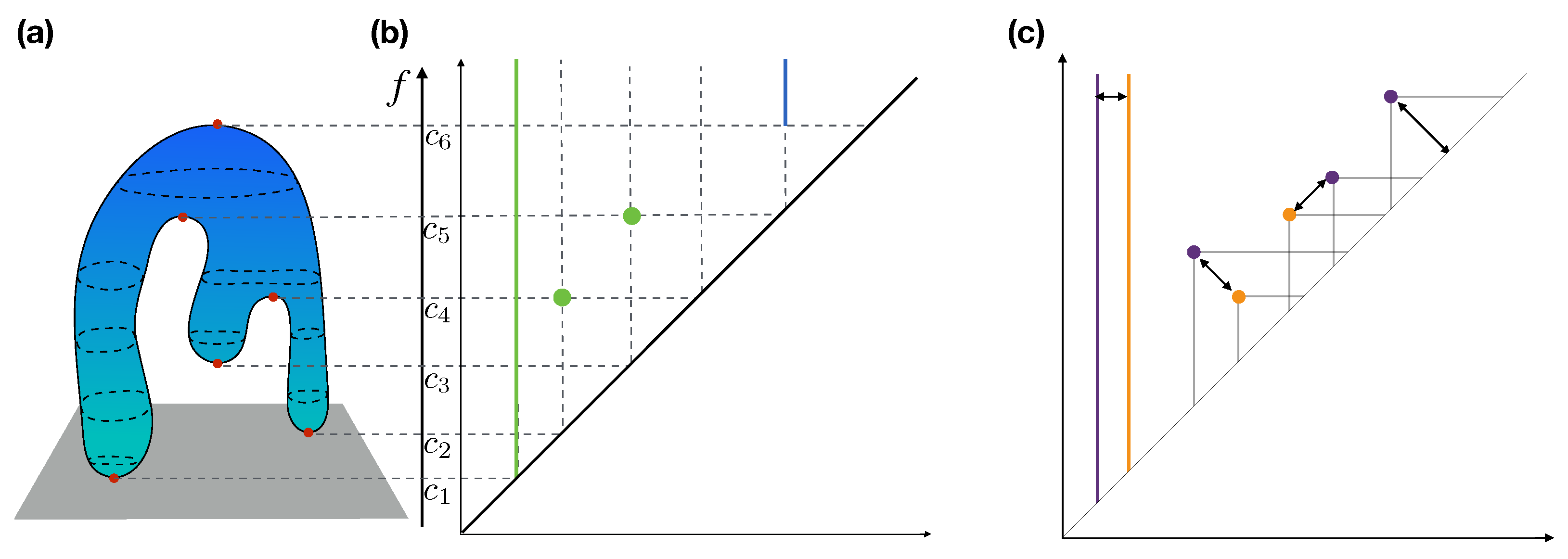
Figure 1, we show how considering a topological sphere
filtered by the height function
yields a persistence diagram whose points correspond to the maxima and minima of
X with respect to the vertical axis. We refer the reader to [
39] for details on topological persistence and persistent homology.
We choose to frame our work in a more general context than homological persistence, namely
rank-based persistence [
11]. Although topological persistence and persistent homology have been extended in several ways, e.g., [
40,
41,
42,
43,
44], rank-based persistence allows us to work directly in the category of the data of choice, rather than topological spaces. The authors assume an axiomatic standpoint based on the three building blocks of homological persistence mentioned above, and the authors generalize persistence to categories and functors other than topological spaces and homology. Importantly, under a few assumptions, persistence built in the rank-based framework still guarantees fundamental properties such as flexibility (dependence on the filtering function), stability [
45], and robustness [
46]. In this setting, we can work with data types such as images and time series, without intermediary topological constructions. We refer to [
11] for details and provide a list of analogies between classical and rank-based persistence in
Table 1.
3.2. Persistent Features
In the spirit of the aforementioned generalization, ref. [
12] (Section 2.2) introduces the concept of
steady persistent features for weighted graphs.
A weighted graph is a pair
, where
is a graph defined by a set of vertices
V and edges
E, and
f is a function assigning (tuples of) real-valued weights to the edges of
G, in symbols
. The weighting function naturally induces a sublevel set filtration
Let
be the set of all subsets of elements (vertices and edges) of
G. Let
F be a graph-theoretical property, e.g., local degree prevalence, independence. The
persistent feature associated with
F is a Boolean mapping returning true if the property
F holds for a certain subset
and false otherwise. Symmetrically to the topological persistence framework, we evaluate
for every subset of every
. See
Figure 2b. Then, we compute the
steadiness of each subset
s along the filtration by counting subsequent sublevels such that
. As in [
12], we refer to
as the steady persistence of the feature
on
. This construction yields a persistence diagram. See
Figure 2c.
4. Persistence-Based Layers
In the following sections, we first build a persistence-based operator that can act as a filter on grayscale images (the operator can also be applied to RGB images treating each channel independently). This construction follows naturally from the definition of steady persistent function. Then, we discuss the main properties of such operators: locality and equivariance. Finally, we specialize our construction to operate as a pooling layer in a convolutional neural network.
4.1. Persistent Features as Equivariant Filters
Locality and equivariance are crucial features for convolutional neural networks, and in general for any group-equivariant model. Indeed, we have:
- 1.
The intensity of a pixel in a grayscale image carries knowledge only when compared to neighboring pixels;
- 2.
Identical configurations located in different regions of the image (translated) should be recognized as such by the model, as is the case for convolutional neural networks [
47]. Mathematically, a function
f is equivariant with respect to the action of a group
G if
. See [
4,
9,
48,
49] for an overview on and examples of equivariant machine learning models
4.1.1. Locality
In this setting, considering the notion of the persistent feature introduced in
Section 3.2, we think about an image as a graph in which vertices are pixels and edges connecting adjacent pixels. Patches (or windows in a time series) of size
k around a pixel (point) correspond to
k-distance neighborhoods of the vertex associated with such a pixel.
4.1.2. Flexibility
Persistent features require a filtered space to be computed. Thus, after associating a graph to an image (or time series), we define the weighting function
, where
S is the set of all subsets of
and
. Importantly,
f can carry additional information about the original data. For instance, when considering images, one can associate with each vertex the intensity value of its underlying pixel, and leverage this information to compute appropriate weights in a process reminiscent of message passing in graph neural networks [
50]. The weighting function
f induces a sub-level set filtration of the graph associated with each pixel of the image. See
Figure 3a,b for an example.
4.1.3. Equivariance
Once the pair has been associated with our data, the proposed construction is naturally equivariant with respect to translation. Indeed, sublevel set filtrations and persistent features are totally determined by the weights and connectivity of the graphs at each filtration level. It is important to notice that the flexibility of the proposed solution makes it possible to further control the equivariance of the operator. For instance, weighting functions that only depend on pairwise intensity values will generate operators that not only are equivariant with respect to translations, but also to isometries (translation, rotations, reflection, and scaling) of the original data.
4.1.4. Parametrization
We can add parameters to the weighting function
f and the feature
to create operators endowed with more complex equivariance and learnable parameters. Let
be a sublevel of
G naturally induced by the intensity of pixels (edges are added when the vertices they connect are added). We define
as the feature mapping
v to true if more than
m and less than
n pixels in the
k-distance neighborhood of
v have an intensity less than
t.
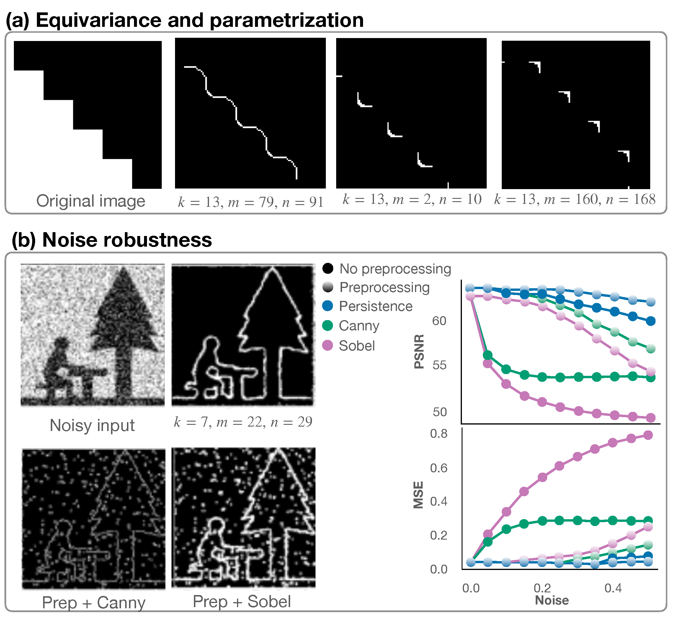
Figure 4a shows how varying parameters
m and
n allow us to highlight radically different aspects of a binary image.
Remark 1.
The operator defined above does not rely on the 2-dimensional structure of the selected patch. Thus, its steady persistence diagram is not only invariant with respect to translations, but also to permutations. This kind of equivariance meshes the standard convolutional equivariance with the fully-connected input/output representation typical of dense layers of an artificial neural network.
4.1.5. Robustness
In the context of both topological and rank-based persistence, robustness means that small changes in the image do not give rise to significant perturbations of the corresponding persistence diagram. This concept is defined in [
12] for persistent features and dubbed
balancedness. In [
51], it is formally shown that
is a
balanced feature in the sense of [
12]. Robustness to noise is showcased in
Figure 4b. Additionally, and in line with the principles of functional data analysis [
52], the proposed operator is adapted to work on continuous data and multiple resolutions: salient features are maintained across different resolutions, as shown in [
53] in the context of persistent images; in computational experiments, the authors demonstrate how downsampling the persistence diagram does not affect the classification accuracy.
4.2. A Steady, Persistent-Feature Layer
The filter
and its steady persistence introduced in
Section 4.1 is endowed with features inherited from its mathematical foundation, which make it suitable for tackling typical machine learning tasks:
- 1.
enhances the signal in correspondence of abrupt changes (a max-pooling filter could be blind to such features);
- 2.
The steady persistence yields invariant representations of the input with respect to the group of isometry;
- 3.
Salt-and-pepper noise does not impair the quality of detected features.
These properties motivate implementing and testing as a complement to pooling and convolutional operators in standard artificial neural networks. In the following paragraphs, we discuss the implementation of a pooling layer with learnable parameters based on persistence features. The same operator can be easily adapted to work as a convolution-like layer.
4.2.1. Persistence-Based Pooling
We consider an image
I and split it in a collection of patches
of size
. For every pixel
, we compute
for some fixed values of
and
k (padding is added if needed). This procedure, which computationally boils down to sorting and slicing operations, yields a persistence diagram with a point per pixel in
. Indeed, we compute the operator
for every
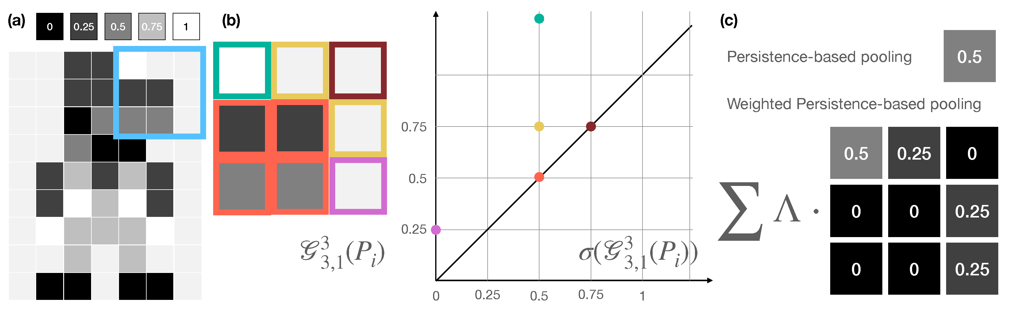
, padding the patch whenever necessary. Symmetrically to the classical max-pooling operator, the maximum persistence—i.e., the distance from the diagonal—shall determine the value to be associated with the entire patch and its downsampling. As an example, see
Figure 5a,b, and the top row of (c).
4.2.2. Parametrization
Alternatively, and following the idea of learnable pooling operators, e.g., [
13], we propose to learn weights
to modulate the contribution of the non-zero component of the persistence diagram, as depicted in
Figure 5c. Because the persistence value associated with each pixel is continuous and
is balanced, it is possible to learn such weights through standard backpropagation.
5. Computational Experiments
We assess the performance of the suggested pooling layer, embedding it into two neural architectures. First, we compare the performance of the persistence-based pooling with some classical pooling implementations. Then, we compute saliency maps (projections of the network’s gradients onto the input images) to highlight qualitative differences across the considered pooling layers.
5.1. Datasets
We perform computational experiments on the MNIST [
54], Fashion-MNIST [
55], and CIFAR-10 [
56] datasets. The MNIST and Fashion-MNIST datasets are composed of grayscale images labeled according to ten classes of hand-written digits and fashion articles, respectively. Both datasets are composed of 60,000, 28 by 28 pixels, black and white images for training, and 10,000 for testing. The CIFAR-10 dataset is composed of 50,000, 32 pixels by 32 pixels, RGB images for training that belong to ten classes: airplane, automobile, bird, cat, deer, dog, frog, horse, ship, and truck. The test is performed on 10,000 additional labeled images.
5.2. Architectures
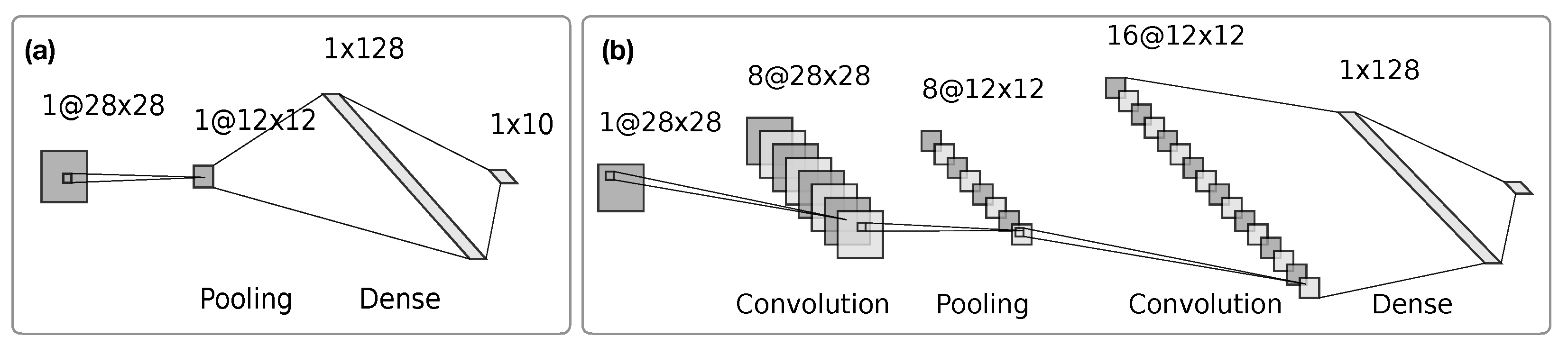
We test the proposed layer via two neural network architectures depicted in
Figure 6. We designed the first architecture to provide the simplest configuration, in which different pooling operators could be compared during a supervised task where parameters are learned via gradient propagation. The second architecture is more akin to the standard convolutional neural network topology in a simple image-classification task; we alternate the convolutional and pooling layers before a dense classifier is provided.
Training
We use sparse categorical cross-entropy as a loss function [
57]. Optimization is conducted in batches of 32 images through the ADAM optimizer [
58] with a learning rate of
. We train each model for 100 epochs and make use of early stopping [
59] with parameters
and
.
5.3. Results
We tested the architectures presented in
Section 5.2 on image classification on the MNIST, Fashion-MNIST, and CIFAR-10 datasets. We adapted the persistence-based and convolutional layers to work with the RGB images of CIFAR-10. Specifically, the persistence-based pooling layer treats channels independently; thus, multiple channels are processed in parallel, ignoring their interactions.
5.3.1. Performance
We compared the performance of several pooling layers, namely:
Additionally, we considered a combination between the learnable persistence-based pooling and max-pooling layers. The two pooling approaches are combined by adding the value obtained through max-pooling on a specific patch to the weighted sum defined in
Section 4.2 and depicted in
Figure 5c. In this way, the weights learned during training combine and modulate the contribution of persistent features detected in each patch and the maximum intensity value of the pixels therein.
We quantify the performance of each network through a standard accuracy metric. We list the results in
Table 2. The proposed layers, outperform the max-pooling and LEAP on both datasets and architectures. The combination of max- and persistence-based-pooling realizes the maximum performance in three out of six experiments. We believe this result points to the complementarity of the two approaches.
5.3.2. Qualitative Comparison of Salient Features
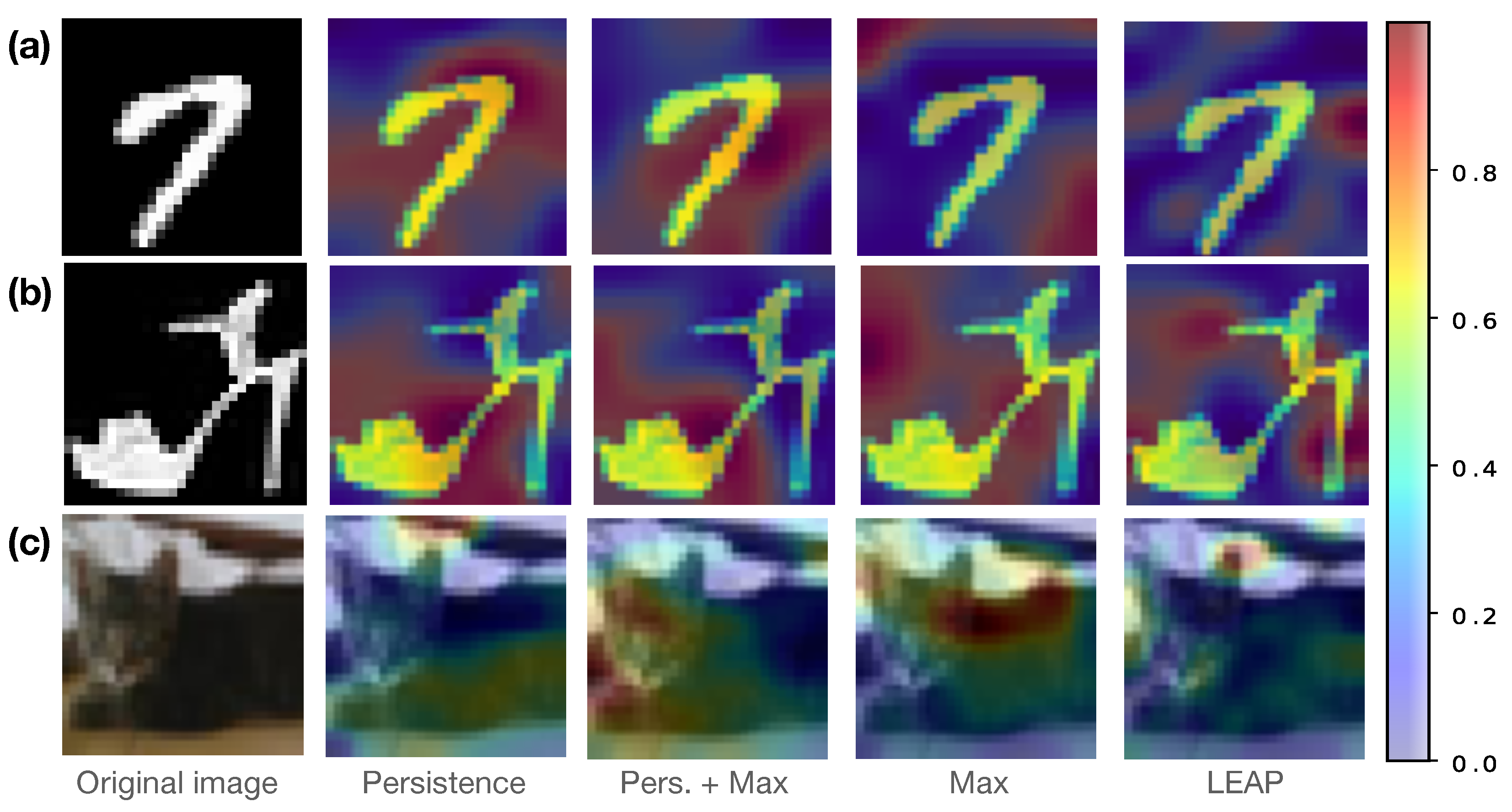
Pooling operators aim to select salient features of their input. Grad-CAM heatmaps [
60] are a visualization tool for highlighting regions of the input that contributed most to the model’s prediction.
Figure 7 showcases Grad-CAM heatmaps obtained through the considered architectures on random input samples. As expected, the persistence-based pooling and its combination with max-pooling yield similar yet distinct heatmaps. In particular, although non-topological, the persistence-based pooling seems to capture geometrical and topological features of the images, such as corners and regions that would cause the foreground image to disconnect. See
Figure 7a,b, respectively.
6. Conclusions
At the crossroad between artificial intelligence and generalizations of topological data analysis, we propose original constructions of neural network layers, taking advantage of the formalism of rank-based persistence. Building on persistent features, we define a convolution-like operator that can be tailored to specific tasks by imposing equivariance through simple invariants. Such invariants can be defined easily by considering features of the data at hand rather than mapping data to the category of topological spaces. Thanks to its mathematical foundation relying on steady persistence and inherited by persistent homology, the proposed operators enjoy mathematically guaranteed properties such as noise robustness and stability to perturbations. We showcase these properties by explicitly defining an image filter operator, relying on steady persistence and testing it in an edge-detection task on noisy images. We compare the performance of the proposed filter against state-of-the-art edge detectors, namely Canny and Sobel operators, comparing the mean squared error and peak signal-to-noise ratio achieved by the three methods on images affected by the salt and pepper noise. In our tests, the proposed operator outperforms competitors in detecting edges and image restoration (noise removal).
Locality, equivariance, and robustness to noise make the proposed class of operators a plausible complement to existing neural layers. Indeed, neural network layers are designed to be as agnostic as possible to the intrinsic properties of their input data. These features make them incredibly general and, at the same time, challenging to constrain to specific data features. This generality induces problematic behaviors and hinders the intelligibility of neural networks’ learning patterns [
61,
62,
63]. The proposed persistence-based layers, allowing the user to select relevant (persistent) features
a priori, pave the road to the design and implementation of hybrid strategies leveraging the data-driven, learnable nature of artificial neural networks and the flexibility of the persistence-based approach.
We devise and implement a special class of the persistent-features-based layer called persistent-based pooling. The proposed layer uses the previously defined edge detection operator to act as a pooling layer in convolutional neural networks. A natural choice of operation for persistence-based pooling is to consider the maximum persistence realized in the diagram associated with each input image patch. We implement an alternative parametrized version that is equipped with learnable weights and easily combinable with standard max-pooling. We test this learnable layer version in image classification on three benchmark datasets. We compare the classification accuracy achieved by our layers with max-pooling and LEAP and embed the pooling layer into two neural architectures (dense and convolutional, respectively). Persistence-based pooling realizes a better performance than its competitors across architectures and datasets. Finally, utilizing Grad-CAM heatmaps, we visualize salient features of input samples to provide a qualitative comparison across the considered pooling layers. There, the persistence-based pooling seems to retrieve relevant geometrical properties of the images.
This approach meshes well with the framework developed in [
64], where inputs, outputs, and weights of a neural network layer are expressed as functions on smooth or discrete spaces. There, we demonstrated how several classes of
linear neural network layers can be expressed as a combination of the function pullback (from a smaller to a larger space), pointwise multiplication of functions, and integration along fibers. We believe that, by combining the two approaches, it will be possible to define general parametric nonlinear layers, where the architecture is defined through the
parametric spans introduced in [
64], whereas the geometry-aware nonlinear computation descends from the methods developed here.
Author Contributions
Conceptualization, M.G.B., M.F., A.M. and P.V.; methodology, M.G.B., M.F. and P.V.; software, validation, data curation, M.G.B. and A.M.; writing—original draft preparation, M.G.B.; writing—review and editing, M.G.B., M.F., A.M. and P.V.; supervision, M.F. All authors have read and agreed to the published version of the manuscript.
Funding
This research received no external funding.
Data Availability Statement
Acknowledgments
We thank Maurizio Sanarico for the useful discussions. Work performed under the auspices of INdAM-GNSAGA.
Conflicts of Interest
The authors declare no conflict of interest.
References
- Narodytska, N.; Kasiviswanathan, S.P. Simple Black-Box Adversarial Attacks on Deep Neural Networks. In Proceedings of the CVPR Workshops, Honolulu, HI, USA, 21–26 July 2017; Volume 2, p. 2. [Google Scholar]
- Van Dyk, D.A.; Meng, X.L. The art of data augmentation. J. Comput. Graph. Stat. 2001, 10, 1–50. [Google Scholar] [CrossRef]
- Thomas, N.; Smidt, T.; Kearnes, S.; Yang, L.; Li, L.; Kohlhoff, K.; Riley, P. Tensor field networks: Rotation-and translation-equivariant neural networks for 3d point clouds. arXiv 2018, arXiv:1802.08219. [Google Scholar]
- Satorras, V.G.; Hoogeboom, E.; Welling, M. E (n) equivariant graph neural networks. In Proceedings of the International Conference on Machine Learning, Virtual, 18–24 July 2021; pp. 9323–9332. [Google Scholar]
- Bergomi, M.G.; Ferri, M.; Zuffi, L. Topological graph persistence. Commun. Appl. Ind. Math. 2020, 11, 72–87. [Google Scholar] [CrossRef]
- Horak, D.; Maletić, S.; Rajković, M. Persistent homology of complex networks. J. Stat. Mech. Theory Exp. 2009, 2009, P03034. [Google Scholar] [CrossRef] [Green Version]
- Hajij, M.; Wang, B.; Scheidegger, C.; Rosen, P. Visual detection of structural changes in time-varying graphs using persistent homology. In Proceedings of the 2018 IEEE Pacific Visualization Symposium (Pacificvis), Kobe, Japan, 10–13 April 2018; IEEE: Piscataway, NJ, USA, 2018; pp. 125–134. [Google Scholar]
- Cang, Z.; Wei, G.W. Integration of element specific persistent homology and machine learning for protein-ligand binding affinity prediction. Int. J. Numer. Methods Biomed. Eng. 2018, 34, e2914. [Google Scholar] [CrossRef]
- Bergomi, M.G.; Frosini, P.; Giorgi, D.; Quercioli, N. Towards a topological–geometrical theory of group equivariant non-expansive operators for data analysis and machine learning. Nat. Mach. Intell. 2019, 1, 423–433. [Google Scholar] [CrossRef] [Green Version]
- Pun, C.S.; Lee, S.X.; Xia, K. Persistent-homology-based machine learning: A survey and a comparative study. Artif. Intell. Rev. 2022, 55, 5169–5213. [Google Scholar] [CrossRef]
- Bergomi, M.G.; Vertechi, P. Rank-based Persistence. Theory Appl. Categ. 2020, 35, 34. [Google Scholar]
- Bergomi, M.G.; Ferri, M.; Tavaglione, A. Steady and ranging sets in graph persistence. J. Appl. Comput. Topol. 2023, 7, 33–56. [Google Scholar] [CrossRef]
- Sun, M.; Song, Z.; Jiang, X.; Pan, J.; Pang, Y. Learning pooling for convolutional neural network. Neurocomputing 2017, 224, 96–104. [Google Scholar] [CrossRef]
- Chowdhury, S.; Mémoli, F. Metric structures on networks and applications. In Proceedings of the 2015 53rd Annual Allerton Conference on Communication, Control, and Computing (Allerton), Monticello, IL, USA, 29 September–2 October 2015; IEEE: Piscataway, NJ, USA, 2015; pp. 1470–1472. [Google Scholar]
- Chowdhury, S.; Mémoli, F. Distances between directed networks and applications. In Proceedings of the 2016 IEEE International Conference on Acoustics, Speech and Signal Processing (ICASSP), Shanghai, China, 20–25 March 2016; IEEE: Piscataway, NJ, USA, 2016; pp. 6420–6424. [Google Scholar]
- Chowdhury, S.; Mémoli, F. Persistent homology of directed networks. In Proceedings of the 2016 50th Asilomar Conference on Signals, Systems and Computers, Pacific Grove, CA, USA, 6–9 November 2016; IEEE: Piscataway, NJ, USA, 2016; pp. 77–81. [Google Scholar]
- Chowdhury, S.; Mémoli, F. A functorial Dowker theorem and persistent homology of asymmetric networks. J. Appl. Comput. Topol. 2018, 2, 115–175. [Google Scholar] [CrossRef] [Green Version]
- Chowdhury, S.; Mémoli, F. Persistent path homology of directed networks. In Proceedings of the Twenty-Ninth Annual ACM-SIAM Symposium on Discrete Algorithms, New Orleans, LA, USA, 7–10 January 2018; SIAM: Philadelphia, PA, USA, 2018; pp. 1152–1169. [Google Scholar]
- Chowdhury, S.; Mémoli, F. Distances and isomorphism between networks: Stability and convergence of network invariants. J. Appl. Comput. Topol. 2022, 1–119. [Google Scholar] [CrossRef]
- Sizemore, A.; Giusti, C.; Bassett, D.S. Classification of weighted networks through mesoscale homological features. J. Complex Netw. 2017, 5, 245–273. [Google Scholar] [CrossRef] [Green Version]
- Aktas, M.E.; Akbas, E.; Fatmaoui, A.E. Persistence homology of networks: Methods and applications. Appl. Netw. Sci. 2019, 4, 61. [Google Scholar] [CrossRef] [Green Version]
- Rieck, B.; Togninalli, M.; Bock, C.; Moor, M.; Horn, M.; Gumbsch, T.; Borgwardt, K. Neural persistence: A Complexity Measure for Deep Neural Networks Using Algebraic Topology. In Proceedings of the 7th International Conference on Learning Representations, ICLR 2019, New Orleans, LA, USA, 6–9 May 2019. [Google Scholar]
- Liu, Z.; Song, Q.; Zhou, K.; Wang, T.H.; Shan, Y.; Hu, X. Detecting interactions from neural networks via topological analysis. Adv. Neural Inf. Process. Syst. 2020, 33, 6390–6401. [Google Scholar]
- Som, A.; Choi, H.; Ramamurthy, K.N.; Buman, M.P.; Turaga, P. Pi-net: A deep learning approach to extract topological persistence images. In Proceedings of the IEEE/CVF Conference on Computer Vision and Pattern Recognition Workshops, Seattle, WA, USA, 14–19 June 2020; pp. 834–835. [Google Scholar]
- Hofer, C.; Kwitt, R.; Niethammer, M.; Uhl, A. Deep learning with topological signatures. In Proceedings of the Advances in Neural Information Processing Systems 30, 31st Annual Conference on Neural Information Processing Systems (NIPS 2017), Long Beach, CA, USA, 4–9 December 2017. [Google Scholar]
- Carrière, M.; Chazal, F.; Ike, Y.; Lacombe, T.; Royer, M.; Umeda, Y. A General Neural Network Architecture for Persistence Diagrams and Graph Classification. 2019. Available online: https://hal.inria.fr/hal-02105788 (accessed on 27 December 2022).
- Carrière, M.; Chazal, F.; Ike, Y.; Lacombe, T.; Royer, M.; Umeda, Y. Perslay: A neural network layer for persistence diagrams and new graph topological signatures. In Proceedings of the International Conference on Artificial Intelligence and Statistics, Online, 26–28 August 2020; pp. 2786–2796. [Google Scholar]
- Haft-Javaherian, M.; Villiger, M.; Schaffer, C.B.; Nishimura, N.; Golland, P.; Bouma, B.E. A topological encoding convolutional neural network for segmentation of 3D multiphoton images of brain vasculature using persistent homology. In Proceedings of the IEEE/CVF Conference on Computer Vision and Pattern Recognition Workshops, Seattle, WA, USA, 14–19 June 2020; pp. 990–991. [Google Scholar]
- Wong, C.C.; Vong, C.M. Persistent homology based graph convolution network for fine-grained 3d shape segmentation. In Proceedings of the IEEE/CVF International Conference on Computer Vision, Montreal, QC, Canada, 11–17 October 2021; pp. 7098–7107. [Google Scholar]
- Lee, J.; Lee, I.; Kang, J. Self-attention graph pooling. In Proceedings of the International Conference on Machine Learning, Long Beach, CA, USA, 9–15 June 2019; pp. 3734–3743. [Google Scholar]
- Gao, H.; Liu, Y.; Ji, S. Topology-aware graph pooling networks. IEEE Trans. Pattern Anal. Mach. Intell. 2021, 43, 4512–4518. [Google Scholar] [CrossRef]
- Nouranizadeh, A.; Matinkia, M.; Rahmati, M. Topology-Aware Graph Signal Sampling for Pooling in Graph Neural Networks. In Proceedings of the 2021 26th International Computer Conference, Computer Society of Iran (CSICC), Tehran, Iran, 3–4 March 2021; IEEE: Piscataway, NJ, USA, 2021; pp. 1–7. [Google Scholar]
- Bianchi, F.M.; Grattarola, D.; Livi, L.; Alippi, C. Hierarchical representation learning in graph neural networks with node decimation pooling. IEEE Trans. Neural Netw. Learn. Syst. 2022, 33, 2195–2207. [Google Scholar] [CrossRef]
- Bonis, T.; Ovsjanikov, M.; Oudot, S.; Chazal, F. Persistence-based pooling for shape pose recognition. In Proceedings of the Computational Topology in Image Context: 6th International Workshop, CTIC 2016, Marseille, France, 15–17 June 2016; Proceedings 6. Springer: Berlin/Heidelberg, Germany, 2016; pp. 19–29. [Google Scholar]
- Zhao, Q.; Ye, Z.; Chen, C.; Wang, Y. Persistence enhanced graph neural network. In Proceedings of the International Conference on Artificial Intelligence and Statistics, Online, 26–28 August 2020; pp. 2896–2906. [Google Scholar]
- Gabrielsson, R.B.; Nelson, B.J.; Dwaraknath, A.; Skraba, P. A topology layer for machine learning. In Proceedings of the International Conference on Artificial Intelligence and Statistics, Online, 26–28 August 2020; pp. 1553–1563. [Google Scholar]
- Carlsson, G.; Gabrielsson, R.B. Topological approaches to deep learning. In Proceedings of the Topological Data Analysis: The Abel Symposium 2018, Geiranger, Norway, 4–8 June 2018; Springer: Berlin/Heidelberg, Germany, 2020; pp. 119–146. [Google Scholar]
- Bergomi, M.G.; Ferri, M.; Vertechi, P.; Zuffi, L. Beyond topological persistence: Starting from networks. Mathematics 2021, 9, 3079. [Google Scholar] [CrossRef]
- Edelsbrunner, H.; Letscher, D.; Zomorodian, A. Topological persistence and simplification. In Proceedings of the 41st Annual Symposium on Foundations of Computer Science, Redondo Beach, CA, USA, 12–14 November 2000; pp. 454–463. [Google Scholar] [CrossRef]
- Bubenik, P.; Scott, J.A. Categorification of Persistent Homology. Discret. Comput. Geom. 2014, 51, 600–627. [Google Scholar] [CrossRef] [Green Version]
- Lesnick, M. The Theory of the Interleaving Distance on Multidimensional Persistence Modules. Found. Comput. Math. 2015, 15, 613–650. [Google Scholar] [CrossRef] [Green Version]
- Oudot, S.Y. Persistence Theory: From Quiver Representations to Data Analysis; American Mathematical Society: Providence, RI, USA, 2015; Volume 209. [Google Scholar]
- McCleary, A.; Patel, A. Bottleneck stability for generalized persistence diagrams. Proc. Am. Math. Soc. 2020, 148, 3149–3161. [Google Scholar] [CrossRef] [Green Version]
- Govc, D.; Levi, R.; Smith, J.P. Complexes of tournaments, directionality filtrations and persistent homology. J. Appl. Comput. Topol. 2021, 5, 313–337. [Google Scholar] [CrossRef]
- Cohen-Steiner, D.; Edelsbrunner, H.; Harer, J. Stability of Persistence Diagrams. Discret. Comput. Geom. 2007, 37, 103–120. [Google Scholar] [CrossRef] [Green Version]
- Di Fabio, B.; Landi, C. A Mayer–Vietoris formula for persistent homology with an application to shape recognition in the presence of occlusions. Found. Comput. Math. 2011, 11, 499. [Google Scholar] [CrossRef] [Green Version]
- O’Shea, K.; Nash, R. An introduction to convolutional neural networks. arXiv 2015, arXiv:1511.08458. [Google Scholar]
- Smidt, T.E. Euclidean symmetry and equivariance in machine learning. Trends Chem. 2021, 3, 82–85. [Google Scholar] [CrossRef]
- Worrall, D.E.; Garbin, S.J.; Turmukhambetov, D.; Brostow, G.J. Harmonic networks: Deep translation and rotation equivariance. In Proceedings of the IEEE Conference on Computer Vision and Pattern Recognition, Honolulu, HI, USA, 21–26 July 2017; pp. 5028–5037. [Google Scholar]
- Gilmer, J.; Schoenholz, S.S.; Riley, P.F.; Vinyals, O.; Dahl, G.E. Neural message passing for quantum chemistry. In Proceedings of the International Conference on Machine Learning, Sydney, Australia, 6–11 August 2017; pp. 1263–1272. [Google Scholar]
- Mella, A. Non-Topological Persistence for Data Analysis and Machine Learning. Ph.D. Thesis, Alma Mater Studiorum Università di Bologna, Bologna, Italy, 2021. [Google Scholar]
- Li, Z.; Kovachki, N.; Azizzadenesheli, K.; Liu, B.; Bhattacharya, K.; Stuart, A.; Anandkumar, A. Fourier neural operator for parametric partial differential equations. arXiv 2020, arXiv:2010.08895. [Google Scholar]
- Adams, H.; Emerson, T.; Kirby, M.; Neville, R.; Peterson, C.; Shipman, P.; Chepushtanova, S.; Hanson, E.; Motta, F.; Ziegelmeier, L. Persistence images: A stable vector representation of persistent homology. J. Mach. Learn. Res. 2017, 18, 1–35. [Google Scholar]
- Deng, L. The mnist database of handwritten digit images for machine learning research [best of the web]. IEEE Signal Process. Mag. 2012, 29, 141–142. [Google Scholar] [CrossRef]
- Xiao, H.; Rasul, K.; Vollgraf, R. Fashion-MNIST: A Novel Image Dataset for Benchmarking Machine Learning Algorithms. arXiv 2017, arXiv:1708.07747. [Google Scholar]
- Krizhevsky, A.; Hinton, G. Learning Multiple Layers of Features from Tiny Images; Technical Report 0; University of Toronto: Toronto, ON, Canada, 2009. [Google Scholar]
- Chollet, F. Keras. Available online: https://keras.io (accessed on 27 December 2022).
- Kingma, D.P.; Ba, J. Adam: A method for stochastic optimization. arXiv 2014, arXiv:1412.6980. [Google Scholar]
- Prechelt, L. Early stopping-but when? In Neural Networks: Tricks of the Trade; Springer: Berlin/Heidelberg, Germany, 1998; pp. 55–69. [Google Scholar]
- Selvaraju, R.R.; Cogswell, M.; Das, A.; Vedantam, R.; Parikh, D.; Batra, D. Grad-cam: Visual explanations from deep networks via gradient-based localization. In Proceedings of the IEEE International Conference on Computer Vision, Venice, Italy, 22–29 October 2017; pp. 618–626. [Google Scholar]
- Holzinger, A.; Saranti, A.; Molnar, C.; Biecek, P.; Samek, W. Explainable AI methods-a brief overview. In Proceedings of the International Workshop on Extending Explainable AI Beyond Deep Models and Classifiers, Vienna, Austria, 18 July 2020; Springer: Cham, Switzerland, 2022; pp. 13–38. [Google Scholar]
- Angerschmid, A.; Zhou, J.; Theuermann, K.; Chen, F.; Holzinger, A. Fairness and explanation in ai-informed decision making. Mach. Learn. Knowl. Extr. 2022, 4, 556–579. [Google Scholar] [CrossRef]
- Cabitza, F.; Campagner, A.; Malgieri, G.; Natali, C.; Schneeberger, D.; Stoeger, K.; Holzinger, A. Quod erat demonstrandum? Towards a typology of the concept of explanation for the design of explainable AI. Expert Syst. Appl. 2023, 213, 118888. [Google Scholar] [CrossRef]
- Bergomi, M.G.; Vertechi, P. Neural network layers as parametric spans. arXiv 2022, arXiv:2208.00809. [Google Scholar]
Figure 1.
Persistent homology. Let us consider a topological space X and a continuous function . The (homological) critical values of f induce a sub-level set filtration of X. (a) Critical values of the height function on a topological sphere. Sublevels of the filtering function f—namely, , for every —yield a filtration of the topological sphere. (b) Changes in the number of generators of the kth homology groups along the filtration can be represented as a persistence diagram. 0-dimensional holes (connected components) are represented as green points. The void obtained at the last sublevel set gives rise to the blue line. (c) Persistence diagrams can be compared by computing an optimal matching of points. Unmatched points are associated with their projection on the diagonal.
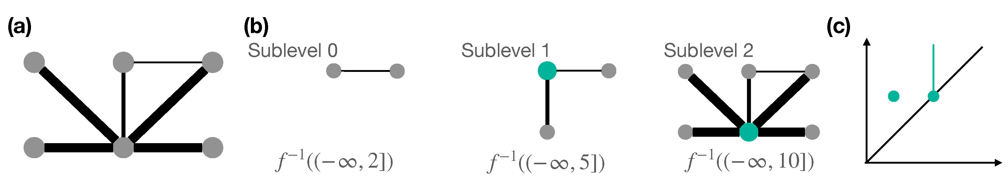
Figure 2.
Persistent features. (a) A weighted graph . The weight values—integers in the set —are encoded as the thickness of the edges. (b) The sublevel set filtration induced by the weights. Teal vertices are the vertices in each sublevel with local degree prevalence. (c) The persistence diagram is obtained by considering the steadiness of each true subset along the filtration. One vertex realizes local degree prevalence at level 5 and stops being prevalent entering level 10. Another vertex is prevalent at level 10 and shall never stop being such because .
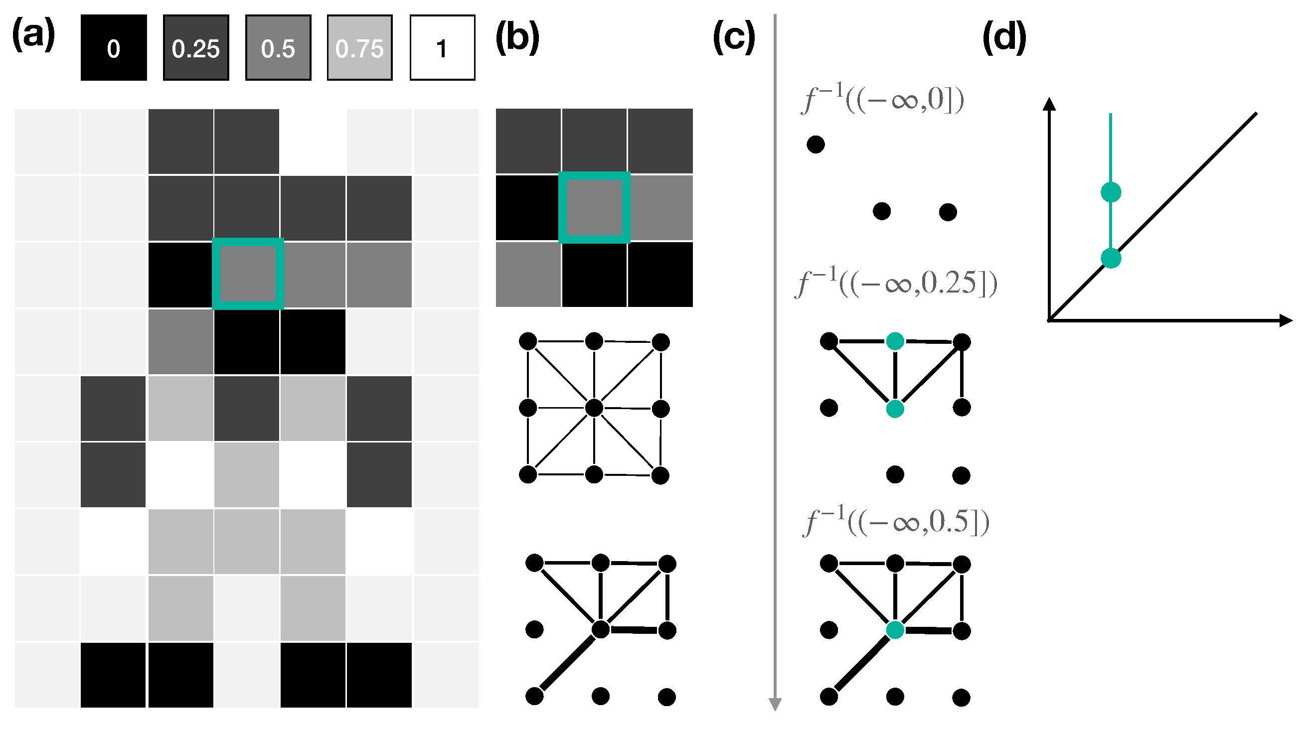
Figure 3.
Persistent features. An image (a) and its interpretation as a weighted graph. (b) Given a focus pixel and its neighborhood (a patch in the example), we map the image to a graph G having as vertices the patch’s pixels and edges connecting adjacent pixels. We weigh edges of G by evaluating the function mapping the intensity values of two vertices to the minimum intensity values of the respective pixels in the image. Edges with weight 0 are not shown. (c) The sublevel-set filtration induced by the weights. Teal vertices are the ones with a prevalent local degree. (d) The persistence diagram obtained considering the filtration/feature pair.
Figure 4.
Persistence-based filter. (a) The persistence-based filter acts in an equivariant fashion (the same feature is recognized throughout the image) and parametrization changes lead to the detection of heterogeneous features. (b) We perform edge detection on a noisy input ( of the pixels are salt and pepper noise). Performance is compared across the proposed persistence-based filter, Canny, and Sobel edge-detection algorithms with and without preprocessing (median filter). Results are showcased for different ratios of noisy pixels. On the right, we compare the Mean Square Error and Peak Signal to Noise Ratio across the considered edge-detection algorithms.
Figure 5.
Persistence-based Pooling. (a) We extract patches of fixed size from the input image. (b) The steady persistence operator yields a persistence diagram associating a persistence value—namely, the distance from the diagonal of the points of the persistence diagram on the right of the panel—with each of the pixels of the considered patch. (c) We associate to each patch either the maximum persistence or a weighted sum of the persistence values associated with each pixel. In the latter case, weights are learned through gradient descent.
Figure 6.
Benchmark architectures. The two architectures used in computational experiments. (a) A toy neural network where a pooling operator is applied directly to input images. The downsampled output of the pooling layer is passed to a dense classifier. In other words, first, the pooled output is flattened, then its dimensionality is reduced to match the number of classes to be predicted by the network. (b) As common practice for CNNs, this architecture alternates convolutional and pooling layers before the dense classifier.
Figure 7.
Grad-CAM heatmaps show pixel-wise saliency of features of an image with respect to the neural network’s gradients. Each row provides an example from a different dataset: MNIST (a), Fashion-MNIST (b), and CIFAR-10 (c).
Figure 7.
Grad-CAM heatmaps show pixel-wise saliency of features of an image with respect to the neural network’s gradients. Each row provides an example from a different dataset: MNIST (a), Fashion-MNIST (b), and CIFAR-10 (c).
Table 1.
Analogy between the classical and rank-based persistence frameworks.
Table 1.
Analogy between the classical and rank-based persistence frameworks.
| Classical Framework | Categorical Framework |
|---|
| Topological spaces | Arbitrary source category |
| Vector spaces | Regular target category |
| Dimension | Rank function on |
| Homology functor | Arbitrary functor from to |
| Filtration of topological spaces | -indexed diagram in |
Table 2.
The accuracy realized by the selected architectures when endowed with ours and state-of-the-art pooling layers.
Table 2.
The accuracy realized by the selected architectures when endowed with ours and state-of-the-art pooling layers.
| Architecture-Dataset | Max | LEAP | PL (Ours) | PML (Ours) |
|---|
| (a)—MNIST | 0.8905 | 0.9238 | | 0.9087 |
| (b)—MNIST | 0.9886 | 0.9848 | | 0.9880 |
| (a)—FMNIST | 0.7978 | 0.8385 | 0.8424 | |
| (b)—FMNIST | 0.8845 | 0.8776 | 0.8930 | |
| (a)—CIFAR-10 | 0.3226 | 0.3291 | | 0.3869 |
| (b)—CIFAR-10 | 0.6145 | 0.5217 | 0.6355 | |
| Disclaimer/Publisher’s Note: The statements, opinions and data contained in all publications are solely those of the individual author(s) and contributor(s) and not of MDPI and/or the editor(s). MDPI and/or the editor(s) disclaim responsibility for any injury to people or property resulting from any ideas, methods, instructions or products referred to in the content. |
© 2023 by the authors. Licensee MDPI, Basel, Switzerland. This article is an open access article distributed under the terms and conditions of the Creative Commons Attribution (CC BY) license (https://creativecommons.org/licenses/by/4.0/).


