
A Novel Framework for Fast Feature Selection Based on Multi-Stage Correlation Measures

 ,
,
Abstract
:1. Introduction
- The use of a cascade of Mutual Information Correlation (MIC) algorithms and the Pearson Correlation to balance speed with accuracy in the process of feature selection;
- A search strategy based in the MIC Score to remove irrelevant and redundant features by a novel combination of the previous algorithms;
- All this packed in a framework for easy deployment and use.
2. Background
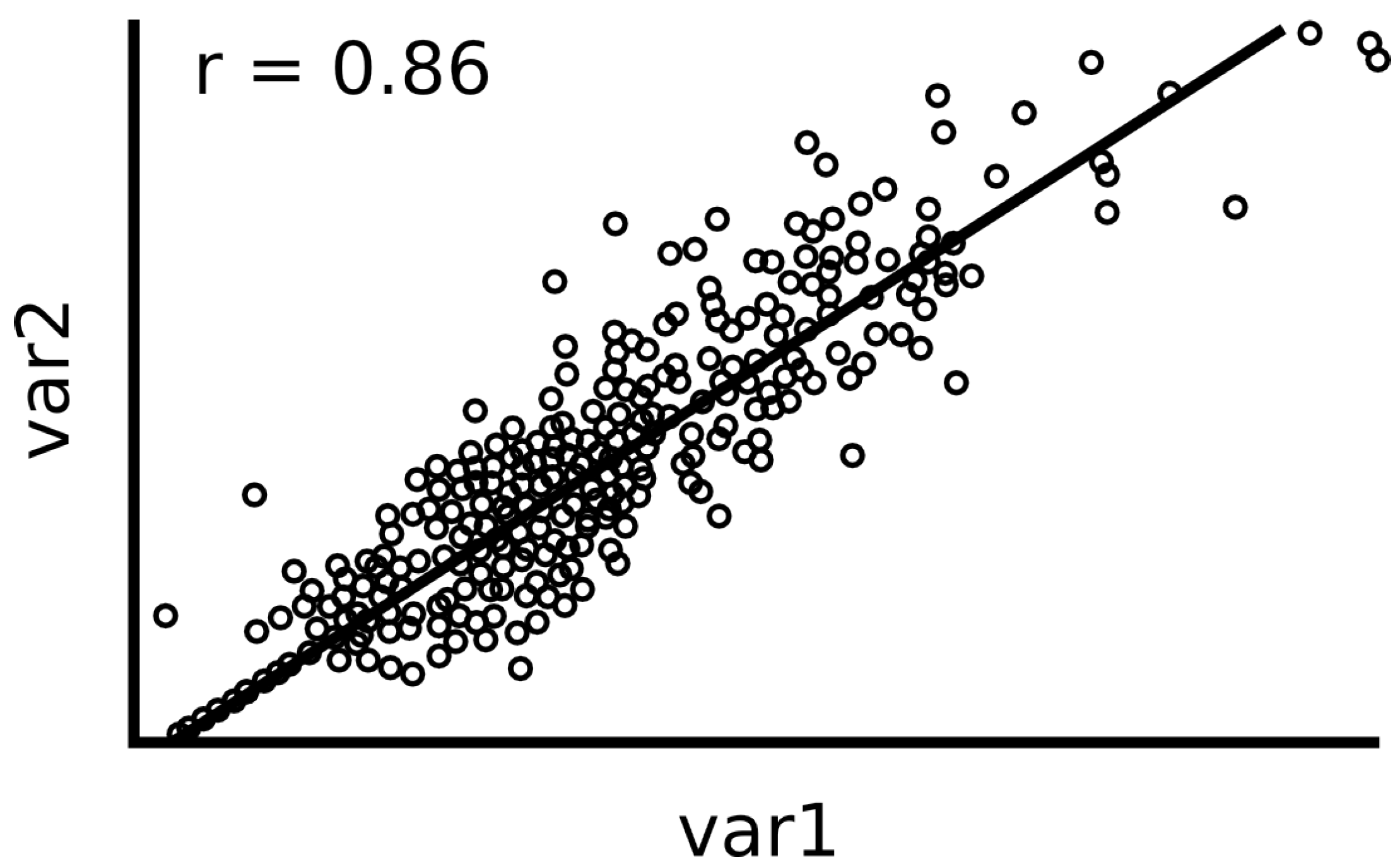
2.1. Pearson Correlation
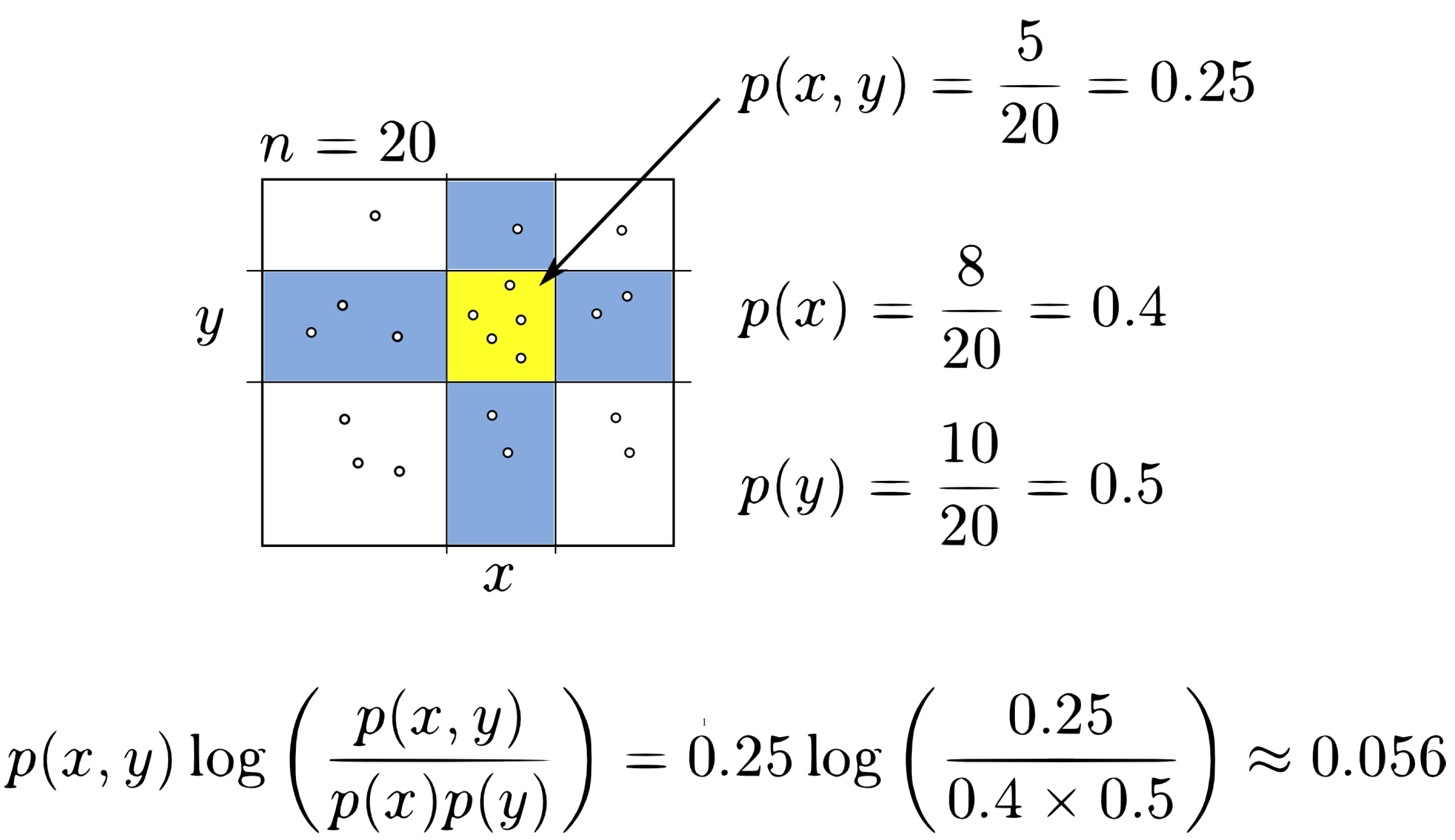
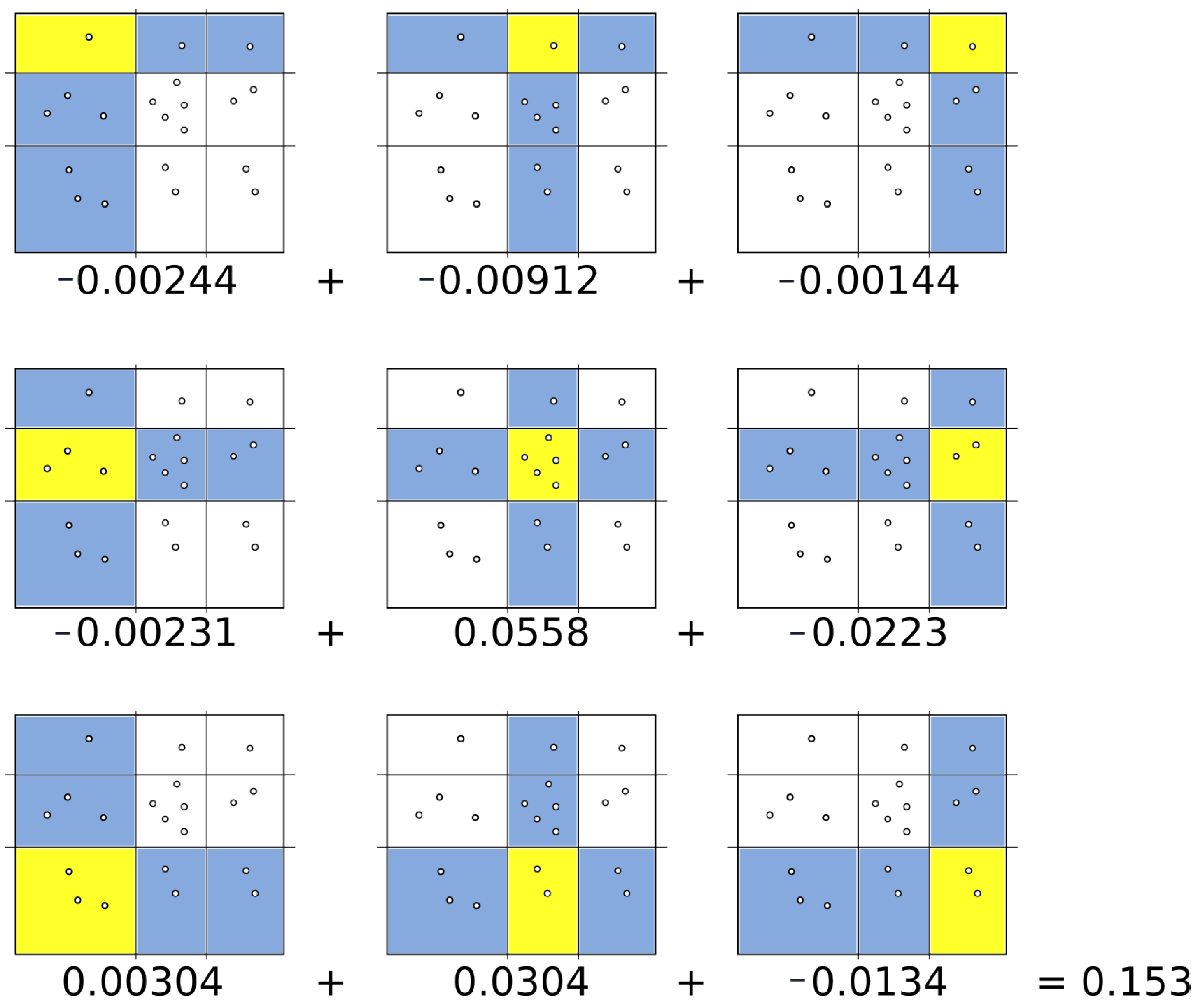
2.2. Mutual Information (MI)
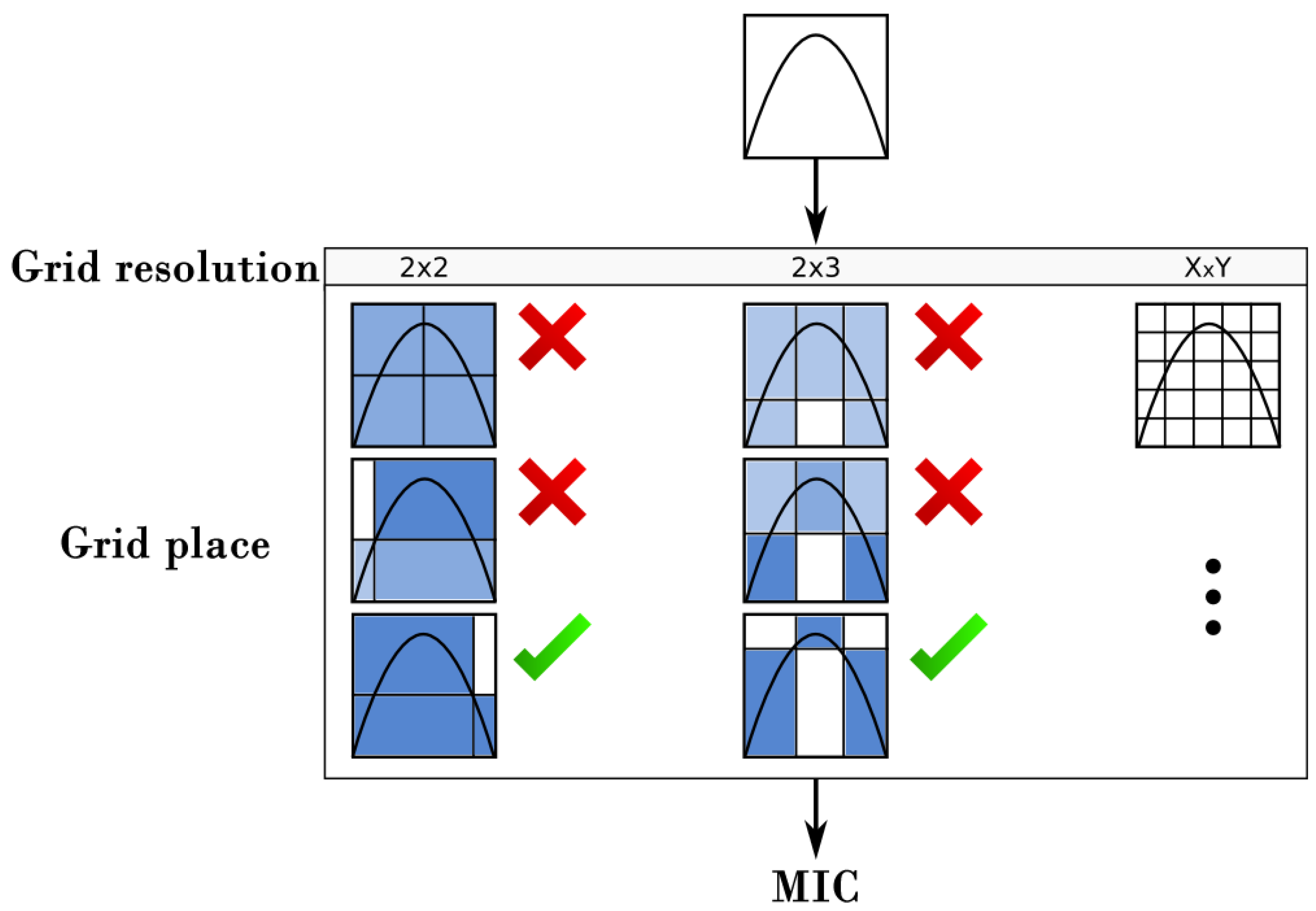
2.3. Maximal Information Coefficient
2.4. Fast and Accurate MIC Estimation
2.4.1. ApproxMaxMI
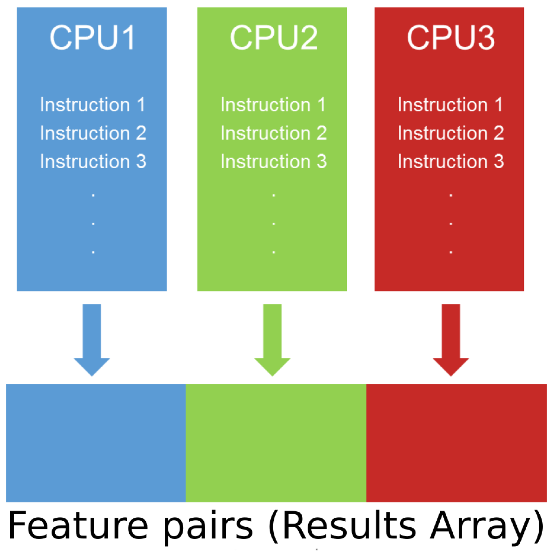
2.4.2. ParallelMIC
2.5. SAMIC
- Set temperature and equipartition grid in both axes;
- Compute the mutual information score of the current grid placement;
- Generate a random neighboring grid placement and compute its new score (more neighbors can be generated at this step if more precision is needed);
- Compare both and :
- If , then .
- If , generate a random choice and make if and only if .
- Update temperature where c is a cooling factor between 0; and
- Repeat steps 2 to 6 until .
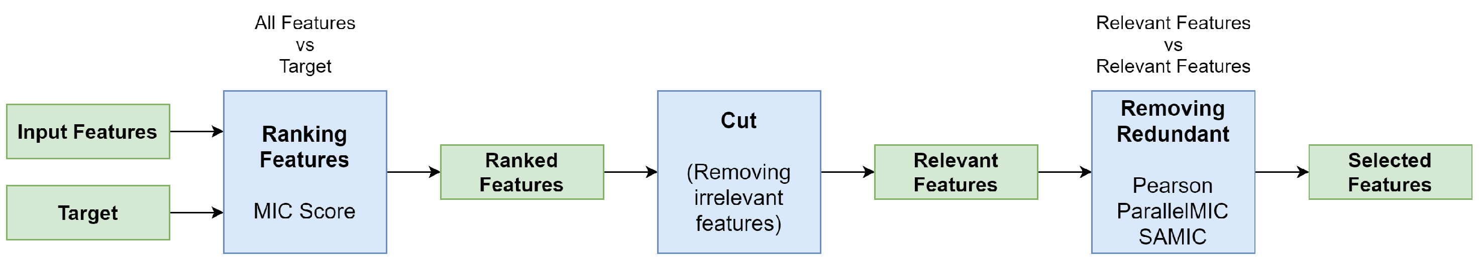
3. A Novel Approach for Feature Selection
- First, feature are ranked by the ParallelMIC score (Section 2.3). This is done to be able to select possible relevant features;
- Second, these features are pruned by the use of cut strategies to remove the irrelevant ones (Section 3.3). Although this allows us to remove irrelevant features, it is necessary to remove redundant features that can provide the same information;
- Third, the use of the Pearson Correlation, ParallelMIC and SAMIC to remove the redundant features at the pipeline by the use of mutual information (Section 3.1) and the idea of clustering.
3.1. Ranking Features
| Algorithm 1: SAMIC One Pair |
 |
3.2. Removing Irrelevant Features
- Cut based in a selected number of features. It returns the n best features according to MIC {, …}, where n is a number selected by the user;
- Cut based on biggest distance correlation. It compares the score of every variable with the subsequent and makes the cut where the biggest difference between them is presented;
- Cut based on the best evaluation using classifiers. In addition to the last two methods R these techniques use classifiers algorithms in order to compare subsets given by cuts, then selects the best of them;
- -
- Cut distance with validation. This cut method is based on the biggest distance correlation. Then, it generates multiple subsets based on the n-biggest score difference and selects the best of them using a classifier;
- -
- Binary Cut. This method tries to reach an optimal cut using binary search over the set R returning the best subset according to a particular classifier;
- -
- Optimal Cut. It is based on a selected number of features, red but in this case n change its value in every iteration from 1 to x and returns the best subset according to the selected classifier.
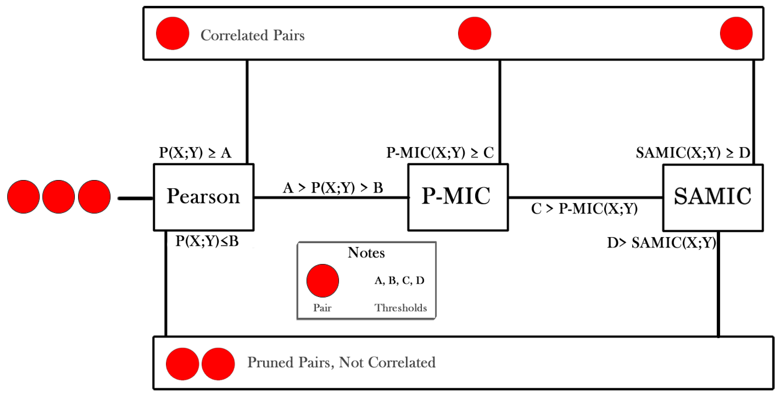
3.3. Removing Redundant Features
- Pearson Correlation.
- ParallelMIC.
- SAMIC.
| Algorithm 2: MIC Estimation Sequence |
 |
| Algorithm 3: Detect Groups |
 |
| Algorithm 4: Feature Selection |
 |
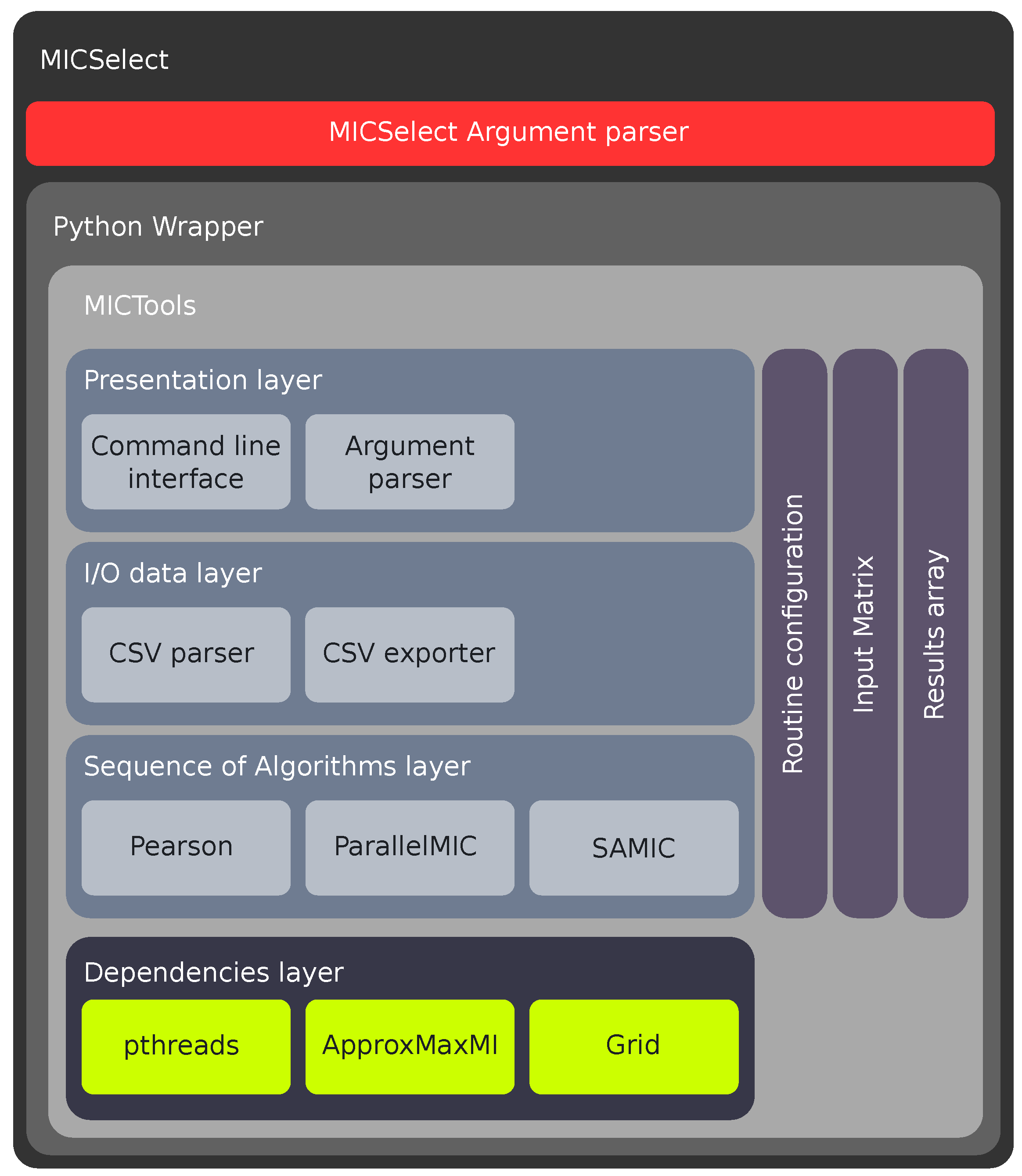
4. MICTools and MICSelect Software Architecture
4.1. MICSelect Layer
4.2. Python Wrapper Layer
- Instructions passing from MICSelect to MICTools;
- Results parsing to Python standard data structures;
- Automatic handling of memory allocation.
4.3. MICTools Layer
4.3.1. Presentation Layer
4.3.2. I/O Layer
4.3.3. Sequence of Algorithms Layer
4.3.4. Dependencies Layer
4.4. MICTools Auxiliary Data Structures
4.4.1. Execution Configuration
4.4.2. Mutual Input Matrix
4.4.3. Array of Results
5. Results & Evaluations
6. Conclusions
Author Contributions
Funding
Institutional Review Board Statement
Informed Consent Statement
Data Availability Statement
Conflicts of Interest
References
- Siddiqa, A.; Karim, A.; Gani, A. Big data storage technologies: A survey. Front. Inf. Technol. Electron. Eng. 2017, 18, 1040–1070. [Google Scholar] [CrossRef] [Green Version]
- Lim, C.K.; Nirantar, S.; Yew, W.S.; Poh, C.L. Novel modalities in DNA data storage. Trends Biotechnol. 2021, 39, 990–1003. [Google Scholar] [CrossRef]
- Oakden-Rayner, L. Exploring large-scale public medical image datasets. Acad. Radiol. 2020, 27, 106–112. [Google Scholar] [CrossRef] [Green Version]
- Chao, G.; Luo, Y.; Ding, W. Recent advances in supervised dimension reduction: A survey. Mach. Learn. Knowl. Extr. 2019, 1, 341–358. [Google Scholar] [CrossRef] [Green Version]
- Reshef, D.N.; Reshef, Y.A.; Finucane, H.K.; Grossman, S.R.; McVean, G.; Turnbaugh, P.J.; Lander, E.S.; Mitzenmacher, M.; Sabeti, P.C. Detecting novel associations in large data sets. Science 2011, 334, 1518–1524. [Google Scholar] [CrossRef] [Green Version]
- Dash, M.; Liu, H.; Motoda, H. Consistency based feature selection. In Proceedings of the Pacific-Asia Conference on Knowledge Discovery and Data Mining, Kyoto, Japan, 18–20 April 2000; Springer: Berlin/Heidelberg, Germany, 2000; pp. 98–109. [Google Scholar]
- Liul, H.; Motoda, H.; Dash, M. A monotonic measure for optimal feature selection. In Proceedings of the 10th European Conference on Machine Learning, Chemnitz, Germany, 21–23 April 1998; Springer: Berlin/Heidelberg, Germany, 1998; pp. 101–106. [Google Scholar]
- McCoy, J.T.; Auret, L. Machine learning applications in minerals processing: A review. Miner. Eng. 2019, 132, 95–109. [Google Scholar] [CrossRef]
- Libbrecht, M.W.; Noble, W.S. Machine learning applications in genetics and genomics. Nat. Rev. Genet. 2015, 16, 321–332. [Google Scholar] [CrossRef] [Green Version]
- Sun, H.; Burton, H.V.; Huang, H. Machine learning applications for building structural design and performance assessment: State-of-the-art review. J. Build. Eng. 2021, 33, 101816. [Google Scholar] [CrossRef]
- Bishop, C.M. Pattern Recognition and Machine Learning (Information Science and Statistics); Springer: Secaucus, NJ, USA, 2006. [Google Scholar]
- Hastie, T.; Tibshirani, R.; Friedman, J. The Elements of Statistical Learning: Data Mining, Inference, and Prediction, 2nd ed.; Springer Series in Statistics; Springer: New York, NY, USA, 2009. [Google Scholar]
- Kumar, V.; Minz, S. Feature selection: A literature review. SmartCR 2014, 4, 211–229. [Google Scholar] [CrossRef]
- Pearson, K. LIII. On lines and planes of closest fit to systems of points in space. London Edinburgh Dublin Philos. Mag. J. Sci. 1901, 2, 559–572. [Google Scholar] [CrossRef] [Green Version]
- Britain, R.S.G. Proceedings of the Royal Society of London; Taylor & Francis: Abingdon, UK, 1895. [Google Scholar]
- Fisher, R.A. The use of multiple measurements in taxonomic problems. Ann. Eugen. 1936, 7, 179–188. [Google Scholar] [CrossRef]
- Rao, C.R. The utilization of multiple measurements in problems of biological classification. J. R. Stat. Soc. Ser. Methodol. 1948, 10, 159–203. [Google Scholar] [CrossRef]
- Roweis, S.T.; Saul, L.K. Nonlinear dimensionality reduction by locally linear embedding. Science 2000, 290, 2323–2326. [Google Scholar] [CrossRef] [Green Version]
- Balasubramanian, M.; Schwartz, E.L.; Tenenbaum, J.B.; de Silva, V.; Langford, J.C. The isomap algorithm and topological stability. Science 2002, 295, 7. [Google Scholar] [CrossRef] [PubMed] [Green Version]
- Belkin, M.; Niyogi, P. Laplacian eigenmaps for dimensionality reduction and data representation. Neural Comput. 2003, 15, 1373–1396. [Google Scholar] [CrossRef] [Green Version]
- Peng, H.; Long, F.; Ding, C. Feature selection based on mutual information criteria of max-dependency, max-relevance, and min-redundancy. IEEE Trans. Pattern Anal. Mach. Intell. 2005, 27, 1226–1238. [Google Scholar] [CrossRef] [PubMed]
- Maaten, L.v.d.; Hinton, G. Visualizing data using t-SNE. J. Mach. Learn. Res. 2008, 9, 2579–2605. [Google Scholar]
- McInnes, L.; Healy, J.; Melville, J. Umap: Uniform manifold approximation and projection for dimension reduction. arXiv 2018, arXiv:1802.03426. [Google Scholar]
- Bolón-Canedo, V.; Sánchez-Maroño, N.; Alonso-Betanzos, A. A review of feature selection methods on synthetic data. Knowl. Inf. Syst. 2013, 34, 483–519. [Google Scholar] [CrossRef]
- Mengle, S.S.; Goharian, N. Ambiguity measure feature-selection algorithm. J. Am. Soc. Inf. Sci. Technol. 2009, 60, 1037–1050. [Google Scholar] [CrossRef]
- Liping, W. Feature selection algorithm based on conditional dynamic mutual information. Int. J. Smart Sens. Intell. Syst. 2015, 8, 316–337. [Google Scholar] [CrossRef] [Green Version]
- Shin, K.; Xu, X.M. Consistency-based feature selection. In Proceedings of the International Conference on Knowledge-Based and Intelligent Information and Engineering Systems, Santiago, Chile, 28–30 September 2009; Springer: Berlin/Heidelberg, Germany, 2009; pp. 342–350. [Google Scholar]
- Benesty, J.; Chen, J.; Huang, Y.; Cohen, I. Pearson correlation coefficient. In Noise Reduction in Speech Processing; Springer: Berlin/Heidelberg, Germany, 2009; pp. 1–4. [Google Scholar]
- Clark, M. A Comparison of Correlation Measures; Center for Social Research, University of Notre Dame: Notre Dame, IN, USA, 2013; Volume 4. [Google Scholar]
- Kinney, J.B.; Atwal, G.S. Equitability, mutual information, and the maximal information coefficient. Proc. Natl. Acad. Sci. USA 2014, 111, 3354–3359. [Google Scholar] [CrossRef] [Green Version]
- Gray, R.M. Entropy and Information Theory; Springer: New York, NY, USA, 1990. [Google Scholar]
- Albanese, D.; Filosi, M.; Visintainer, R.; Riccadonna, S.; Jurman, G.; Furlanello, C. Minerva and minepy: A C engine for the MINE suite and its R, Python and MATLAB wrappers. Bioinformatics 2012, 29, bts707. [Google Scholar] [CrossRef] [PubMed] [Green Version]
- Tang, D.; Wang, M.; Zheng, W.; Wang, H. RapidMic: Rapid Computation of the Maximal Information Coefficient. Evol. Bioinform. Online 2014, 10, 11. [Google Scholar] [CrossRef] [Green Version]
- Kirkpatrick, S. Optimization by simulated annealing: Quantitative studies. J. Stat. Phys. 1984, 34, 975–986. [Google Scholar] [CrossRef]
- Yu, L.; Liu, H. Feature selection for high-dimensional data: A fast correlation-based filter solution. In Proceedings of the 20th International Conference on Machine Learning (ICML-03), Washington, DC, USA, 21–24 August 2003; pp. 856–863. [Google Scholar]
- Herlihy, M.; Shavit, N. The Art of Multiprocessor Programming; Morgan Kaufmann Publishers Inc.: San Francisco, CA, USA, 2008. [Google Scholar]
- Williams, A. C++ Concurrency in Action: Practical Multithreading; Manning Pubs Co Series; Manning: Shelter Island, NY, USA, 2012. [Google Scholar]
- Hennessy, J.L.; Patterson, D.A. Computer Architecture: A Quantitative Approach, 5th ed.; Morgan Kaufmann Publishers Inc.: San Francisco, CA, USA, 2011. [Google Scholar]
- Dua, D.; Graff, C. UCI Machine Learning Repository 2017. Available online: https://archive.ics.uci.edu/ml/index.php (accessed on 15 June 2021).
- Chang, C.C.; Lin, C.J. LIBSVM: A library for support vector machines. ACM Trans. Intell. Syst. Technol. 2011, 2, 27:1–27:27. Available online: http://www.csie.ntu.edu.tw/~cjlin/libsvm (accessed on 1 June 2021). [CrossRef]
- Yamada, Y.; Lindenbaum, O.; Negahban, S.; Kluger, Y. Feature Selection using Stochastic Gates. Proc. Mach. Learn. Syst. 2020, 2020, 8952–8963. [Google Scholar]
- Rogers, J.; Gunn, S. Identifying feature relevance using a random forest. In International Statistical and Optimization Perspectives Workshop “Subspace, Latent Structure and Feature Selection"; Springer: Berlin/Heidelberg, Germany, 2005; pp. 173–184. [Google Scholar]
- Bonidia, R.P.; Machida, J.S.; Negri, T.C.; Alves, W.A.L.; Kashiwabara, A.Y.; Domingues, D.S.; De Carvalho, A.; Paschoal, A.R.; Sanches, D.S. A Novel Decomposing Model With Evolutionary Algorithms for Feature Selection in Long Non-Coding RNAs. IEEE Access 2020, 8, 181683–181697. [Google Scholar] [CrossRef]
- Pedregosa, F.; Varoquaux, G.; Gramfort, A.; Michel, V.; Thirion, B.; Grisel, O.; Blondel, M.; Prettenhofer, P.; Weiss, R.; Dubourg, V. Scikit-learn: Machine Learning in Python. J. Mach. Learn. Res. 2011, 12, 2825–2830. [Google Scholar]


| Dataset | RAPIDMIC | ParallelMIC |
|---|---|---|
| Spellman | 1060.649 | 889.538 |
| MLB2008 | 350.142 | 262.95 |
| MICSelect Options | |||
|---|---|---|---|
| Short Command | Value | Range | Description |
| Mandatory Options | |||
| -i | Path | Input CSV file. | |
| -y | String | Target Name of dataset. | |
| Not mandatory options | |||
| -r | Remove redundant features. | ||
| -x | Integer | [0, 4] | Step wise feature selection |
| -s | Integer | [1, N] | Static cut, gives the number of features selected sorted by importance. N is the total number of features in the dataset. |
| -w | Write features correlation in a file. | ||
| MICTools Options | ||||
|---|---|---|---|---|
| Short Command | Long Command | Value | Range | Description |
| General options | ||||
| -a | –alpha | Double | (0, 1] | Alpha value for MIC calculations. |
| -i | –input | String | Input CSV file. | |
| -o | –output | String | Output results file. | |
| -f | –keys_file | String | Filter keys file. Restricts the generated pairs to be constructed only with those variables present in the file. | |
| -g | –target | String | Name of the variable against which all of the remaining variables will be paired. | |
| -h | –header | Indicates that the input file contains a Header line. | ||
| -t | –max_threads | Integer | >0 | Max number of threads to use during the computation. |
| -d | –default | Forces the program to run Pearson, ParallelMIC and SAMIC using their default parameters. | ||
| Analysis options | ||||
| -P | –Pearson | Includes Pearson in the analysis schedule. | ||
| -R | –ParallelMIC | Includes ParallelMIC in the analysis schedule. | ||
| -S | –SAMIC | Includes SAMIC in the analysis schedule. | ||
| RapidMIC options | ||||
| -u | –clumps | Double | >0 | Number of clumps (must be larger than 0). |
| -p | –min_pearson | Double | [0, 1] | Sets ParallelMIC to compute only those pairs whose Pearson coefficient absolute value is above the given value. |
| -e | –max_pearson | Double | [0, 1] | Sets ParallelMIC to compute only those pairs whose Pearson coefficient absolute value is below the given value. |
| SAMIC options | ||||
| -n | –neighbors | Integer | >0 | SAMIC amount of candidate neighbors to consider for each temperature of the simulated annealing stage. |
| -c | –cooling | Double | (0, 1) | Temperature cooling factor to be usesd in SAMIC. |
| -m | –min_temp | Double | (0, 1) | Minimum temperature value to be used in SAMIC. |
| -j | –min_parallelmic | Double | [0, 1] | SAMIC min ParallelMIC value. Restricts computation to pairs with ParallelMIC score above the given value. |
| -k | –max_parallelmic | Double | [0, 1] | SAMIC max ParalllMIC value. Restricts computation to pairs with ParallelMIC score below the given value. |
| Algorithm | Abbreviation | Main Parameters |
|---|---|---|
| Logistic Regression | LR | penalty: l2 solver: lbfgs max_iter: 100 random_state: 0 multi_class: auto |
| K-NearestNeighbor | KNN | n_neighbors: 3 algoithm: auto metric: minkowski leaf_size: 30 |
| Suport Vector Classifier | SVC | kernel: rbf max_iter: no limit gamma: scale C (regularization parameter): 1 |
| Prop. Top 10 | STG | Random F. | M1-GA | |||||
|---|---|---|---|---|---|---|---|---|
| Dataset Name | AUC | Time | AUC | Time | AUC | Time | AUC | Time |
| SPECTF Heart | 0.77 | 0.006 | 0.76 | 3.445 | 0.78 | 0.061 | 0.74 | 379 |
| Cervical Cancer (R.F.) | 0.93 | 0.012 | 0.82 | 4.376 | 0..58 | 0.066 | 0.94 | 639 |
| Breast Cancer (Diag.) | 0.92 | 0.488 | 0.81 | 4.053 | 0.88 | 0.067 | 0.78 | 2642 |
| Breast Cancer (Prog.) | 0.74 | 0.023 | 0.6 | 4.321 | 0.59 | 0.07 | 0.62 | 1340 |
| Sports articles | 0.79 | 0.164 | 0.83 | 4.709 | 0.79 | 0.116 | 0.82 | 9686 |
| Lung Cancer | 0.82 | 0.001 | 0.9 | 3.359 | 0.57 | 0.062 | 0.94 | 7773 |
| HCC Survival | 0.67 | 0.023 | 0.64 | 4.028 | 0.68 | 0.067 | 0.65 | 28345 |
| Duke Breast Cancer | 0.81 | 0.182 | 0.8 | 10.646 | 0.75 | 0.071 | 0.91 | 10915 |
| Colon Cancer | 0.89 | 0.102 | 0.86 | 5.191 | 0.62 | 0.069 | 0.92 | 5046 |
| Leukemia | 0.98 | 0.093 | 0.74 | 10.601 | 0.75 | 0.067 | 0.96 | 15,446 |
| Sonar | 0.70 | 0.127 | 0.78 | 3.539 | 0.81 | 0.072 | 0.78 | 7475 |
| Splice | 0.84 | 0.017 | 0.87 | 4.672 | 0.88 | 0.095 | 0.81 | 781 |
| Average | 0.82 | 0.083 | 0.784 | 5.245 | 0.723 | 0.074 | 0.823 | 7539 |
| Prop. Top 10 Features | |||||
|---|---|---|---|---|---|
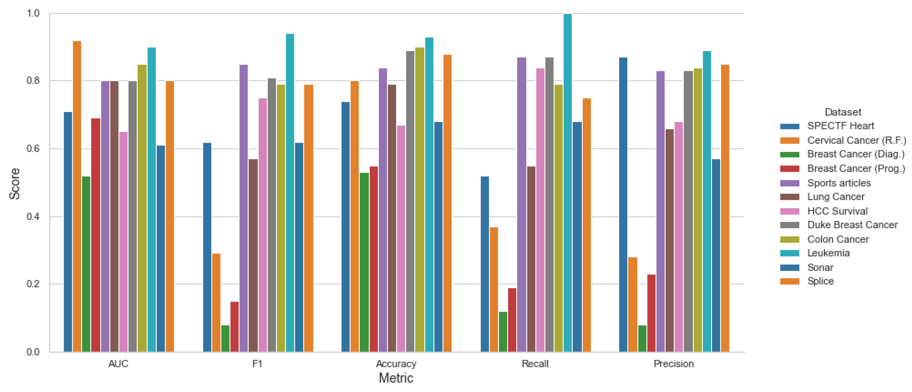
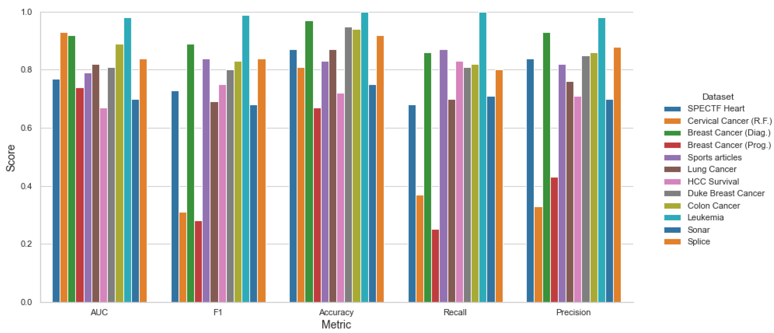
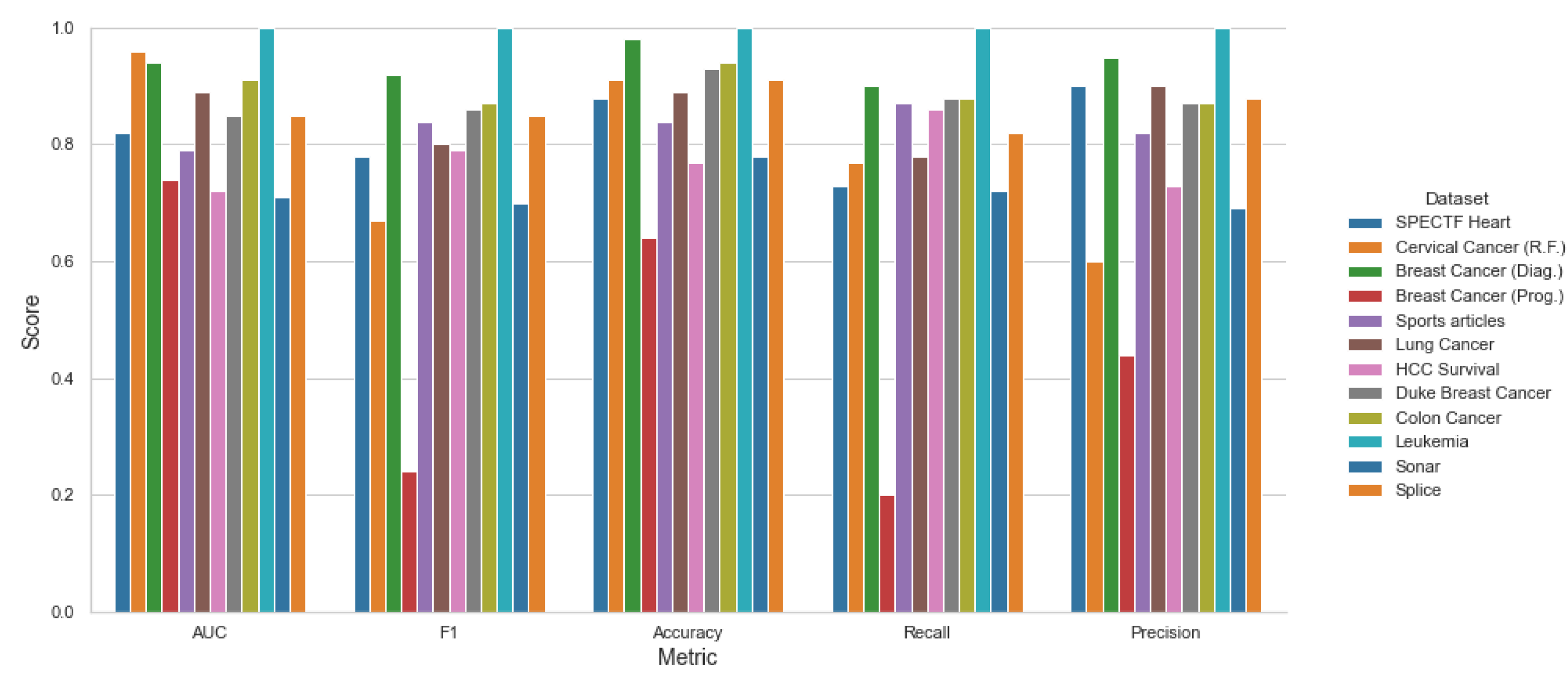
| Dataset Name | AUC | F1 | Accuracy | Recall | Precision |
| SPECTF Heart | 0.77 ± 0.10 | 0.73 ± 0.13 | 0.87 ± 0.10 | 0.68 ± 0.19 | 0.84 ± 0.13 |
| Cer. Cancer (R.F.) | 0.93 ± 0.03 | 0.31 ± 0.31 | 0.81 ± 0.15 | 0.37 ± 0.38 | 0.33 ± 0.33 |
| B. Cancer (Diag.) | 0.92 ± 0.03 | 0.89 ± 0.04 | 0.97 ± 0.02 | 0.86 ± 0.08 | 0.93 ± 0.03 |
| B. Cancer (Prog.) | 0.74 ± 0.07 | 0.28 ± 0.18 | 0.67 ± 0.14 | 0.25 ± 0.19 | 0.43 ± 0.33 |
| Sports articles | 0.79 ± 0.05 | 0.84 ± 0.04 | 0.83 ± 0.06 | 0.87 ± 0.06 | 0.82 ± 0.03 |
| Lung Cancer | 0.82 ± 0.12 | 0.69 ± 0.24 | 0.87 ± 0.15 | 0.70 ± 0.29 | 0.76 ± 0.29 |
| HCC Survival | 0.67 ± 0.07 | 0.75 ± 0.08 | 0.72 ± 0.09 | 0.83 ± 0.15 | 0.71 ± 0.09 |
| Duke B. Cancer | 0.81 ± 0.10 | 0.80 ± 0.14 | 0.95 ± 0.05 | 0.81 ± 0.22 | 0.85 ± 0.14 |
| Colon Cancer | 0.89 ± 0.09 | 0.83 ± 0.13 | 0.94 ± 0.08 | 0.82 ± 0.13 | 0.86 ± 0.16 |
| Leukemia | 0.98 ± 0.05 | 0.99 ± 0.03 | 1.00 ± 0 | 1.00 ± 0 | 0.98 ± 0.06 |
| Sonar | 0.70 ± 0.11 | 0.68 ± 0.14 | 0.75 ± 0.14 | 0.71 ± 0.22 | 0.70 ± 0.14 |
| Splice | 0.84 ± 0.04 | 0.84 ± 0.04 | 0.92 ± 0.04 | 0.80 ± 0.06 | 0.88 ± 0.06 |
| Average | 0.82 ± 0.07 | 0.72 ± 0.13 | 0.86 ± 0.09 | 0.73 ± 0.16 | 0.76 ± 0.15 |
Publisher’s Note: MDPI stays neutral with regard to jurisdictional claims in published maps and institutional affiliations. |
© 2022 by the authors. Licensee MDPI, Basel, Switzerland. This article is an open access article distributed under the terms and conditions of the Creative Commons Attribution (CC BY) license (https://creativecommons.org/licenses/by/4.0/).
Share and Cite
Garcia-Ramirez, I.-A.; Calderon-Mora, A.; Mendez-Vazquez, A.; Ortega-Cisneros, S.; Reyes-Amezcua, I. A Novel Framework for Fast Feature Selection Based on Multi-Stage Correlation Measures. Mach. Learn. Knowl. Extr. 2022, 4, 131-149. https://doi.org/10.3390/make4010007
Garcia-Ramirez I-A, Calderon-Mora A, Mendez-Vazquez A, Ortega-Cisneros S, Reyes-Amezcua I. A Novel Framework for Fast Feature Selection Based on Multi-Stage Correlation Measures. Machine Learning and Knowledge Extraction. 2022; 4(1):131-149. https://doi.org/10.3390/make4010007
Chicago/Turabian StyleGarcia-Ramirez, Ivan-Alejandro, Arturo Calderon-Mora, Andres Mendez-Vazquez, Susana Ortega-Cisneros, and Ivan Reyes-Amezcua. 2022. "A Novel Framework for Fast Feature Selection Based on Multi-Stage Correlation Measures" Machine Learning and Knowledge Extraction 4, no. 1: 131-149. https://doi.org/10.3390/make4010007