Article

A Novel Feature Representation for Prediction of Global Horizontal Irradiance Using a Bidirectional Model

1
A.K. Choudhury School of Information Technology, University of Calcutta, Kolkata 700106, India
2
Bangabasi Morning College, University of Calcutta, Kolkata 700009, India
3
Department of Statistics, University of Calcutta, Kolkata 700019, India
4
National Institute of Wind Energy (NIWE), Under the Ministry of New and Renewable Energy, Chennai 600100, India
*
Author to whom correspondence should be addressed.
These authors contributed equally to this work.
Mach. Learn. Knowl. Extr. 2021, 3(4), 946-965; https://doi.org/10.3390/make3040047
Submission received: 21 October 2021 / Revised: 21 November 2021 / Accepted: 23 November 2021 / Published: 25 November 2021
(This article belongs to the Special Issue Recent Advances in Feature Selection)

Abstract

:
Complex weather conditions—in particular clouds—leads to uncertainty in photovoltaic (PV) systems, which makes solar energy prediction very difficult. Currently, in the renewable energy domain, deep-learning-based sequence models have reported better results compared to state-of-the-art machine-learning models. There are quite a few choices of deep-learning architectures, among which Bidirectional Gated Recurrent Unit (BGRU) has apparently not been used earlier in the solar energy domain. In this paper, BGRU was used with a new augmented and bidirectional feature representation. The used BGRU network is more generalized as it can handle unequal lengths of forward and backward context. The proposed model produced 59.21%, 37.47%, and 76.80% better prediction accuracy compared to traditional sequence-based, bidirectional models, and some of the established states-of-the-art models. The testbed considered for evaluation of the model is far more comprehensive and reliable considering the variability in the climatic zones and seasons, as compared to some of the recent studies in India.

1. Introduction

Solar energy is one of the important components of the alternative sources of energy [1]. India is ranked third after China and the United States of America (USA) in terms of solar energy development [2]. Precise prediction of solar energy is very important for several applications, such as electricity grid management, the trading of solar energy, etc. [3,4]. The Global Horizontal Irradiance (GHI) is often taken as a proxy for solar energy generation and used for the prediction task [5,6,7,8,9,10,11,12]. A considerable amount of uncertainty is present in solar energy due to its strong dependence on atmospheric conditions, which makes the prediction task challenging [13,14,15].
In [10], the authors categorized solar forecasting horizons into short-term, medium-term, and long-term forecasting. For one to few hours ahead of solar forecasting, i.e., for short-term forecasting, currently, machine-learning models are the state-of-the-art models [14]. In [16], the authors stated that short-term solar forecasting is essential for balancing demand and supply and decreasing the storage requirement, unit commitment, etc. From the literature study, we found that statistical and Artificial Neural Network (ANN)-based models were effective in intra-hour (short-term) or intra-day (medium-term) solar forecasting.
Many of the current works suggest that deep-learning-based approaches are very suitable for time-series forecasting [5,17,18,19,20,21]. In [22], the authors suggested that, in several application domains, deep learning algorithms dominate machine learning approaches and have a superior ability to learn the non-linear structure between the input and output.
Long Short-Term Memory (LSTM) is one of the deep-learning models, specifically designed to handle sequential data. GRU is a more recent addition to deep-learning-based sequence models, and it simplifies the architecture of LSTM to an extent. In recent papers [5,8,9,23,24,25], the authors used traditional unidirectional LSTM and GRU to forecast solar irradiation, and they demonstrated that both LSTM and GRU dominate standard statistical techniques as well as state-of-the-art machine-learning models. For time-series data, LSTM is most popularly used for intra-hour (short-term) solar forecasting [26]. Subsequently, in some of the recent research papers [27,28], the authors demonstrated that, by replacing traditional LSTM with bidirectional LSTM, they produced better forecasting performance for the energy domain.
A bidirectional deep-learning model is a combination of two sequential layers: one layer is trained with the preceding values, ( t k ) to ( t 1 ) t h term of the sequence, referred to as the past context to predict the t t h term. This is typically called the forward layer. The other layer uses ( t + 1 ) to ( t + k ) t h term of the sequence referred as the future context to predict the t t h term. This is known as the backward layer. The above process is described by taking the window size of k. Both these contexts are available when we are predicting missing values or finding representation of words by context. Understandably for a typical forecasting task, the future context is unavailable. In some of the recent works [27,28], the authors used the same past context as both the past and future context and reported better results.
In this paper, we propose a feature representation, called a bidirectional feature, that augments the past context and uses a simple technique to construct the future context. This representation is further discussed in subsequent sections.
The main contributions of this paper are summarized as follows:
  • Bidirectional GRU is applied for the first time to solar energy forecasting, and it is shown to be better performing than other common sequence models, such as unidirectional LSTM, Bidirectional-LSTM (BLSTM), and Unidirectional GRU.
  • A new feature representation with a bidirectional nature is proposed, which further augments the performance of BGRU. The model shows improved performance compared to two state-of-the-art models.
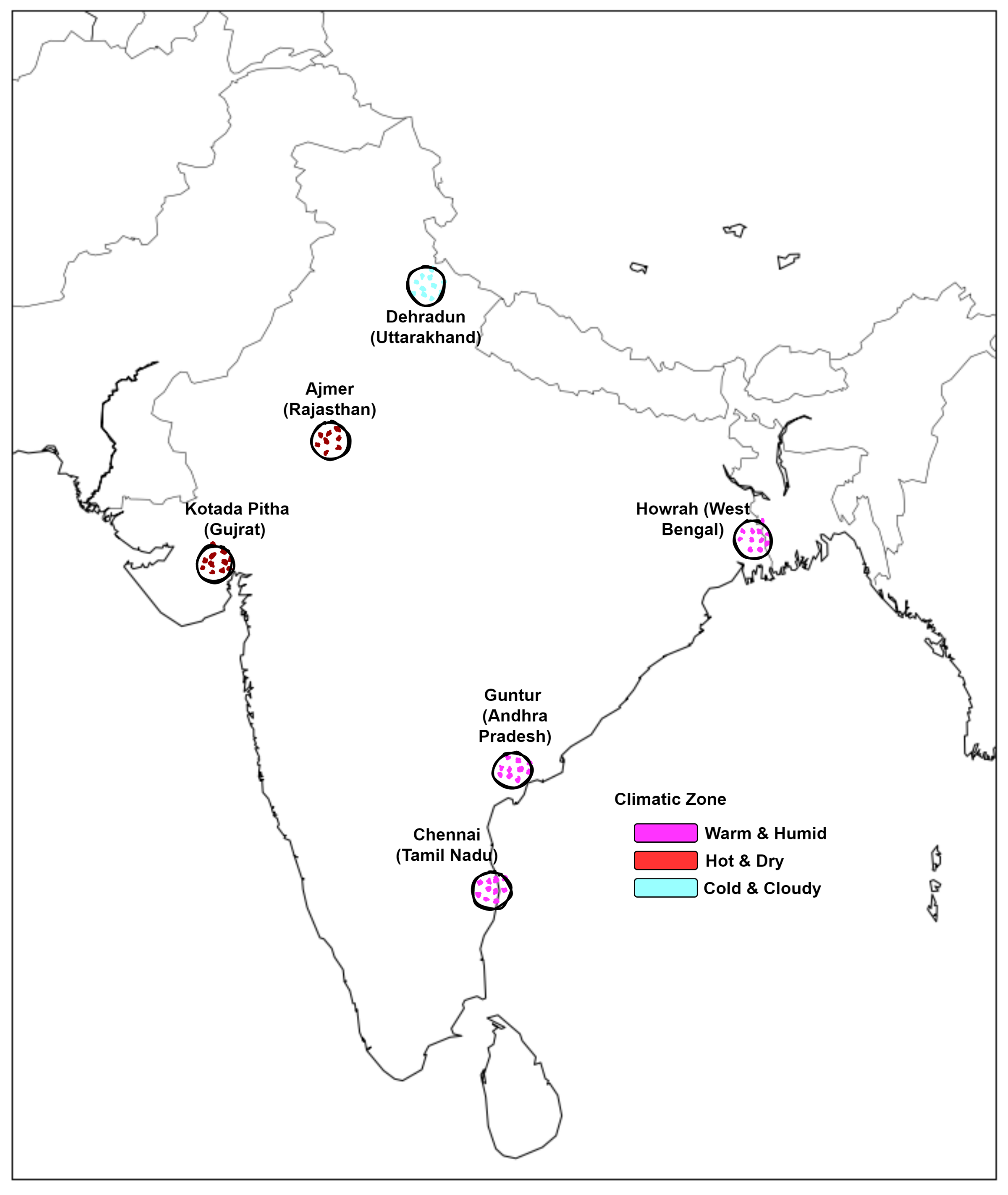
  • The performance of the model is validated on real-life data from six solar stations from three climatic zones and in two seasons in India.
The rest of the paper is organized as follows. In Section 2, the recent forecasting models for renewable energy are outlined. In Section 3, the detailed architecture of BLSTM and BGRU with the proposed bidirectional feature representation are elaborated. In Section 4, the materials and methods employed in setting up the empirical study is discussed. In Section 5, the results of the prediction models are presented along with critical analysis and discussion. Finally, in Section 6, our concluding remarks are presented.

2. Forecasting Models for Renewable Energy

In this section, some of the recent research efforts in the domain of renewable energy forecasting are presented. They are classified broadly in the following two categories, namely (a) machine-learning-based models and (b) deep-learning-based models.

2.1. Machine Learning Based Models

In [10], the authors reported that, compared to SVR, decision tree regressor and k-nearest neighbors (kNN), Multilayer Perceptron (MLP) performed the best to forecast solar irradiation for one-hour-ahead prediction. In [29], the authors proposed a unique re-sampling technique to design a uni-variate solar PV power forecasting model using machine learning algorithms for a forecasting horizon of length of five minutes to three hours.
Out of Multi-Layer Perceptron (MLP), Support Vector Regression (SVR), Random Forest (RF), and Multiple Linear Regression (MLR), RF was reported to have the best accuracy compared to the others. In [30], the authors predicted three components of hourly solar irradiation, namely global horizontal, beam normal, and diffuse horizontal for a horizon of 6 h. The authors used three different models, namely smart persistence, ANN and RF. They observed that RF showed the best performance for all three components of solar irradiation.
Some of the approaches can be classified as hybrid using both ANN and ML. As example, In [31] the authors used a radial basis neural network for solar power prediction in the Netherlands, where the parameters were tuned using swarm optimization. In paper [32], the authors advocated the use of an Ensemble model for both wind and solar energy prediction as they can reduce variance of the base learners. It can be observed that most of the research has been conducted for short-term solar forecasting [10,29,30,31]. Currently, RF has been popularly used in certain studies [29,30,32] for short-term solar forecasting.

2.2. Deep-Learning-Based Models

In [5],the authors used LSTM to implement a solar irradiation prediction model. They reported that LSTM outperformed other models, such as ANN, support vector machines (SVM), and autoregressive moving average (ARMA). In [9], the authors proposed a unidirectional LSTM-based day-ahead hourly solar forecasting model to forecast irradiation along with other meteorological features. In [8], an hourly univariate photovoltaic power forecasting model was proposed based on LSTM-RNN.
In [33], the authors reported a day-ahead hybrid PV power forecasting model, where the authors used LSTM and Convolutional neural network (CNN) to build the model. In [34], the authors observed that the LSTM model does not need pre-processing and works best with stateful models. In deep-learning-based approaches, there are also approaches based on CNN, where the authors attempted to focus on the global information unlike the sequence models [35].
It can be observed that, currently, unidirectional LSTM has proved its excellence over many state-of-the-art machine learning as well as statistical models in the context of short-term solar forecasting [5,9,33]. In paper [27], the authors developed a hourly PV power forecasting model. In this context, the authors studied the effectiveness of different time series prediction models divided into two classes statistical (ARMA, ARIMA, SARIMA) and Neural Network (NN)-based models (LSTM, Bidirectional-LSTM).
It has been shown that NN-based models, specifically Bidirectional-LSTM outperformed others. They concluded that, for one-hour-ahead prediction, NN-based models performed considerably well. In [28], the authors proposed a solar power prediction model based on different variants of LSTM and as well as different Bidirectional LSTM variants with two choices of architectures single layer and double layer. The authors claimed that bidirectional LSTM of a single layer outperformed others and also they validated their proposed model against four different seasons.
In Table 1, we summarize the above-discussed research works in terms of several attributes, such as the type of the research data, proposed technique, length of the forecasting window, the country, correctness, and advantages or disadvantages. Recent papers adopted Bidirectional LSTM and reported better results. Nevertheless, we observed that Bidirectional GRU were not applied, and the same set of observations were used for both forward and backward context.

3. Detailed Working of the Deep-Learning-Based Models

This section has two subsections. In the first part, a description of the sequence models is provided. In the second part, the different feature representation options for the sequence models are elaborated. In Section 3.2, the proposed augmented bidirectional feature representation is explained, which is one of the main contributions of the paper.

3.1. Sequential Deep Learning Models

Sequence or ordered data is present in various application domains namely, climate, finance, medical diagnosis, astronomy, bio-informatics, etc. Traditional machine-learning models consider all features to be independently and identically distributed (iid), which do not apply here. Recurrent Neural Networks (RNN) are deep-learning models designed to handle sequence data. In RNN, the next step output is dependent on the current input as well as the previous step output.
This was much better than sequence data but was prone to a problem known as the Vanishing Gradient problem. As a result of which, RNN was incapable of remembering long-term dependency. LSTM [37], is a special type of RNN, where the hidden memory state update is customized through some unique gates. Hence, LSTM shows a better understanding in the case of long-range dependencies and is effective with the vanishing [38] and exploding gradient problem [39].
GRU [40] is mostly similar to LSTM and was proposed by [41]. However, it has some specific advantages over LSTM. GRU is less complicated than LSTM, and it uses fewer parameters compared to LSTM. Hence, it is faster than LSTM. LSTM uses both input and forget gate while GRU performs both these operations using the reset gate. The function of the reset gate is to decide how to combine the current input with the old memory. The update gate decides what amount of previous memory needs to maintain. The equations that govern the working of GRU are given as follows:
R e s e t g a t e ( r t ) = σ ( W r h t 1 + U r X t )
U p d a t e g a t e ( z t ) = σ ( W z h t 1 + U z X t )
C e l l s t a t e ( c t ) = t a n h ( W c ( r t h t 1 ) + U c X t )
N e w s t a t e ( h t ) = ( z t c t ) + ( ( 1 z t ) h t 1 )
Here, X t is the input vector at timestamp t, and σ denotes the sigmoid activation function. h t and h t 1 are the hidden state vectors. W r , W z and W c are the parameter matrices related to hidden state vector h t 1 for reset gate, update gate, and the current cell state. U r , U z , and U c are the parameter matrices related to the input vector X t for reset gate, update gate and the current cell state. ∘ implies element-wise matrix multiplication, and the new state h t is the final output vector.
  • The GRU model, rather than any sequential model, is trained by selecting a continuous portion or window from the input data. Instead of taking all such windows for training, it is often broken into batches.
  • If the batches are considered dependent on each other, then it is called a stateful model.
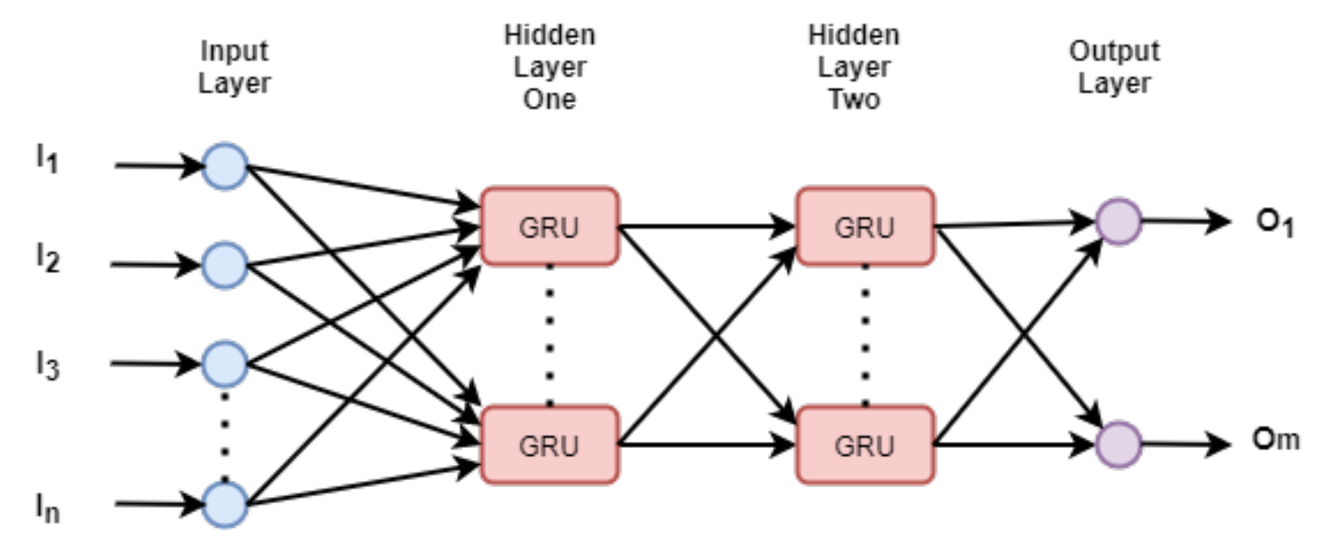
  • Typically, when dealing with the sequence data, the hidden layer nodes are any sequential cells. In Figure 1, a simple schematic diagram of a deep neural network is shown, whereas a basic building block in the hidden layers, the GRU cells are used. The inputs and the outputs are denoted as [ I 1 , I 2 , I 3 , …, I n ], and [ O 1 , …, O m ] respectively.
  • As with traditional neural networks, gradient-descent and back-propagation are used to learn the parameters of the network. Some of the state-of-the-art optimizers are ADAM, RMSProp, Stochastic Gradient Descent [42,43,44], etc.
In the sequence, a few preceding values of the sequence were used to predict the current value. For tasks, such as missing data prediction, suitable text representation, speech recognition, etc., instead of only the preceding sequence, the succeeding sequence data is available. BLSTM [45,46] and BGRU are specifically designed for the same. In Figure 2a, the detailed generic architecture of BGRU is shown where the length of the forward and backward context is identical. In Figure 2b, the length of the forward and backward context is different.
The functionality of BGRU is as follows:
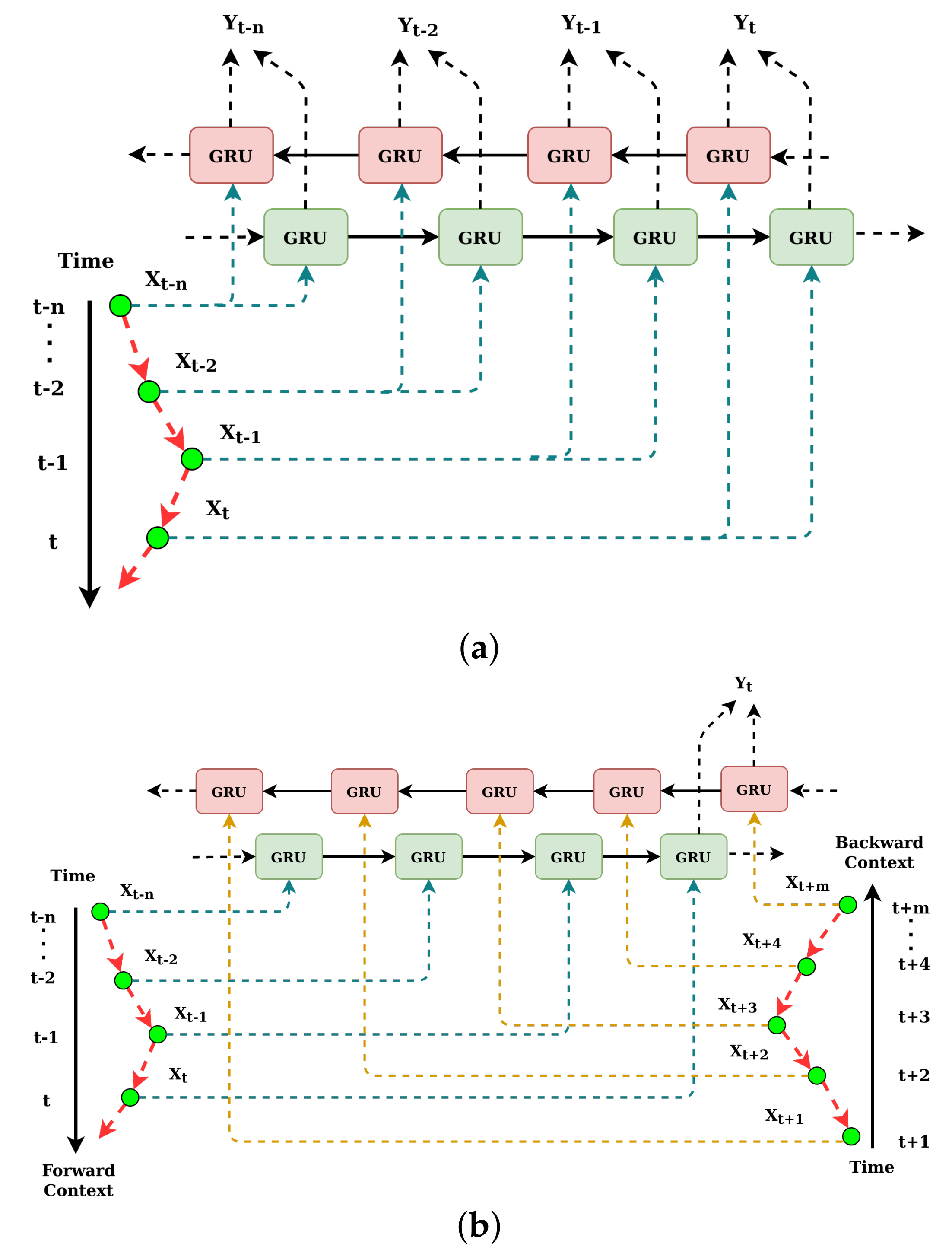
  • BGRU is a fusion of two independent unidirectional GRU layers when one layer maintains the forward hidden states whereas the other maintains the backward hidden states. In the forward pass, BGRU processes inputs sequence as …, X t 3 , X t 2 , X t 1 , X t for the time steps …, t 3 , t 2 , t 1 , t, and, in the backward pass, BGRU processes the input sequence for the time steps t, t 1 , t 2 , t 3 , …in the reverse direction.
  • After both forward and backward passes were completed, the hidden states are concatenated to form a final single set of hidden states.
  • Then, the final hidden states go through a densely connected layer to produce the output sequence as …, y t 3 , y t 2 , y t 1 , y t .

3.2. Feature Preparation for Sequential Models

In this section, four different types of feature representations are explained. The models trained with these different feature representations are named ULSTM (Unidirectional LSTM + Unidirectional Feature), M-ULSTM (Unidirectional LSTM + Augmented Feature), BLSTM, BD-BLSTM (Bidirectional LSTM + Proposed Bidirectional Feature), and BD-BGRU (Bidirectional GRU + Proposed Bidirectional Feature). In Table 2, the models are compared based on several attributes, such as type of the model, feature type, and the input feature representation, and also we explain the generic architecture of each model in the following:
1.
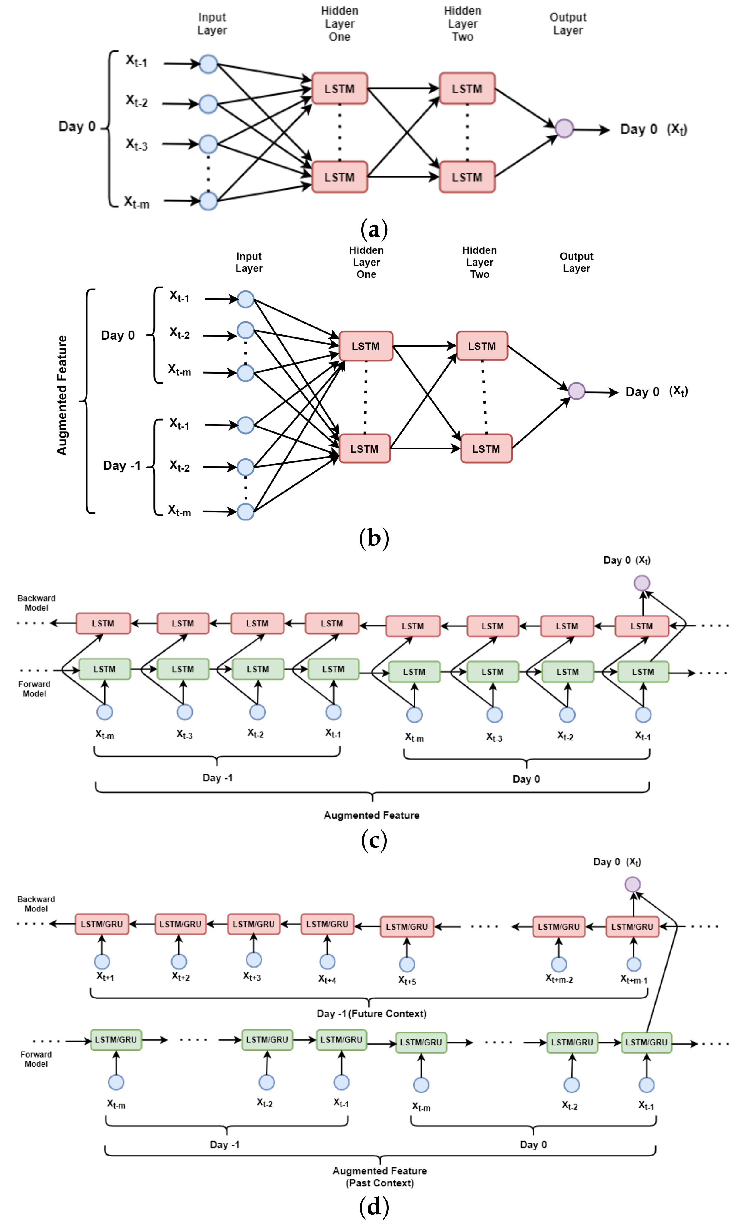
ULSTM: In Figure 3a, the high-level block diagram of ULSTM is presented. In this case, to predict solar irradiation for the time step t as X t , usually, the past context of the same day is used. For example, to predict X t , the input sequence is defined as [ X t m ,…, X t 2 , X t 1 ]. The traditional sliding window approach was used to represent the whole feature set. The length of the window is denoted as m.
2.
M-ULSTM: As with the previous feature representation, this also uses past values, and hence is a unidirectional model. However, the past context is augmented here, with the previous values, corresponding to the same time. In Figure 3b, the high-level block diagram of M-ULSTM is presented. For example, for predicting solar irradiation for the time step t as X t for D a y 0 we not only used the same day past sequence denoted as D a y 0 [ X t m ,…, X t 2 , X t 1 ] but also values from previous day denoted as D a y 1 [ X t m ,…, X t 2 , X t 1 ].
3.
BLSTM: This is the traditional variant of bidirectional LSTM, where the same context is used to train the model both from forward and backward directions. Figure 3 b depicts the block diagram of BLSTM. In this architecture, the same augmented features were used in both the left and right contexts.
4.
BD-BLSTM and BD-BGRU: In the case of time-series prediction problems, such as text data, traditional bidirectional deep-learning models use the same past sequence for both the forward and backward context. In this paper, a simple technique is proposed, first to augment the past context and next to construct future context from previous day. The model used here is more generalized allowing the past and future context to be of unequal length. In Figure 3d, the block diagram of this proposed bidirectional feature set with BLSTM and BGRU is presented. The right or backward context is collected from the previous day denoted as D a y 1 [ X t + 1 ,…, X t + m 2 , X t + m 1 ].
Table 2. Comparison of models with different input feature representations.
ModelsInput SequenceRemarks
ULSTM D a y 0 [ X t m ,…, X t 2 , X t 1 ]Same day m input time steps
M-ULSTMAugmented Feature
{ D a y 1 [ X t m ,…, X t 2 , X t 1 ]
D a y 0 [ X t m ,…, X t 2 , X t 1 ]}
Same day m input time steps are
augmented with previous day
m time steps
BLSTM L c o n t e x t = Augmented Feature
{ D a y 1 [ X t m ,…, X t 2 , X t 1 ]
D a y 0 [ X t m ,…, X t 2 , X t 1 ]}
R c o n t e x t = Augmented Feature
{ D a y 1 [ X t m ,…, X t 2 , X t 1 ]
D a y 0 [ X t m ,…, X t 2 , X t 1 ]}
Same day m input time steps
along with previous day m time steps
is used as both forward
and backward context
BD-BLSTM/
BD-BGRU
L c o n t e x t Augmented Feature
{ D a y 1 [ X t m ,…, X t 2 , X t 1 ]
D a y 0 [ X t m ,…, X t 2 , X t 1 ]}
R c o n t e x t
D a y 1 [ X t + 1 ,…, X t + m 2 , X t + m 1 ]
Same day m input time steps along with
previous day m time steps is used as
forward context and augmented with
previous day m future time
steps as backward context
Figure 3. Schematic diagram of (a) ULSTM (b) M-ULSTM (c) BLSTM (d) BD-BLSTM/BD-BGRU.
Make 03 00047 g003

4. Materials and Methods

This section has five subsections. In the first subsection, how the data is collected and its different characteristics are described. In the second subsection, the pre-processing steps are discussed that are applied to the data. In the third section, the experimental setup of the models is discussed. In the fourth section, the reference models are briefly discussed, and also they been used for comparison, and finally, in the fifth subsection, various performance metrics are enclosed that are employed for evaluation and comparison of the models.

4.1. Data-Set Description

We used the application programming interface (API) provided by the Center for Wind Energy Technology (C-WET) to crawl solar irradiation data for Solar Radiation Resource Assessment (SRRA) stations across India. In this paper, data from 2016 is used for three climatic zones (Hot and Dry, Warm and Humid, and Cold and Cloudy), and six stations located at Chennai (Tamil Nadu), Howrah (West Bengal), Guntur (Andhra Pradesh), Kotada Pitha (Gujrat), and Ajmer (Rajasthan).
Figure 4, depicts solar stations in different climatic zones. Table 3 describes the details of the solar stations, location, etc. For each of the stations, we chose a month each from the rainy and winter season because the rainy season is known for its high variability due to cloud and rain, on the other hand, in winter comparatively, the uncertainty is less. C-WET provides data with a one-minute resolution. In our work, this was aggregated into a five minute resolution.

4.2. Data Pre-Processing

Following pre-processing on the raw data [47]:
1.
For each station–month combination, to remove night hours, only the measurements of GHI between 7 a.m. to 7 p.m. were used.
2.
After that, the GHI values for each day were aggregated into five minutes, and then merged for all the days in a single time-series. The time-series should be formatted as a three-dimensional array, where the three dimensions are the size of the batch, number of time-steps (Window Size), and number of input features. In a single window, 20 time-steps of GHI were used. Batch size refers to the number of training samples used at the time of the training phase for one iteration. We used 100 training samples in a batch. During the learning process, successive batches are used to train the network.
3.
Finally, GHI values were normalized in between [−1,1] using the following transformation (5).
X t ^ = X t X m i n X m a x X m i n

4.3. Experimental Setup

To predict GHI 20 steps (1 h 40 min) ahead, historical solar irradiance data was used. The whole time-series data is decomposed into train and test set with the proportion of 80% and 20%. A subset of training data is used as a validation set (20% of the training set) to validate the model. In this work, different variants of LSTM and GRU architectures were implemented, and the prediction performance is compared against two recent benchmark models. In the following section, the technical details of all implemented models are described briefly.
  • Different architectures of LSTM and GRU were developed using the Keras [48] API in python. For bidirectional models, three hidden layers, and for the traditional LSTM, two hidden layers were used.
  • In the input layer of both LSTM and GRU, different choices of input size, i.e., sequential length were varied from 20 to 60 steps.
  • In the output layer, the 20-time steps were predicted, which is 100 min in this case.
  • For the bidirectional models, two sequential models were applied separately. Prediction were made from the forward direction by one model and from the backward direction by the other model. Finally, by combining both predictions, the actual decision is made.
  • In the output layer, 20 neurons with linear activation were used. For traditional LSTM, the same non-linear activation tanh [49] was used, and in the output layer, linear activation was used.
  • All models are trained on Adaptive Moment Estimation (Adam) [50] optimizer. For all the implemented models, different hyper-parameters [51], such as learning rate, the number of nodes in different hidden layers, batch size, and the number of epochs were optimized using Bayesian Optimization [52] approach. In this context, the Tree-structured Parzen Estimator (TPE) [53] algorithm of Hyperopt [54] package in python is used. In Table 4, the details of all the hyper-parameters were enlisted.

4.4. Comparison with Other Models

The prediction performance of the proposed methods BD-BLSTM and BD-BGRU are compared with two recently published works on solar power forecasting. In the first reference model [29], the authors used RF from the SciKit-learn package [55].
They reported a multi-step ahead prediction model, where RF was applied for each output step individually. It is to be noted, for each RF model, separately, multiple hyper-parameters, such as n_estimators (number of trees in the forest), min_samples_split (minimum number of samples required to split an internal node), and min_samples_leaf (minimum number of samples required to be at a leaf node) were tuned using the Grid Search [56] approach with 10-fold cross-validation. To represent input features for each output step separately, they proposed a unique resampling technique for each RF model. In [8], the authors used the traditional LSTM with two sequential layers to design the forecasting model.
In Table 5, the architectural details of all the reference models and the proposed model are presented. From the table, some notable findings can be made, which are listed as follows:
  • The reference models [8,29], used univariate time series data, such as the proposed model.
  • In [8], the authors used raw time series (Non-stationary) to design the forecasting model, similar to this work.

4.5. Performance Metrics

In Equation (6), the computation of the Normalized Root Mean Squire Error (nRMSE) is shown. nRMSE is known for its scale independence property. G H I t is the t t h actual value, and the corresponding predicted value is represented as G H I t ^ . This always returns a non-negative value. The closer the value to zero, the better is the fit of the model with the data.
nRMSE = i = 1 n ( G H I t G H I t ^ ) 2 n i = 1 n G H I t

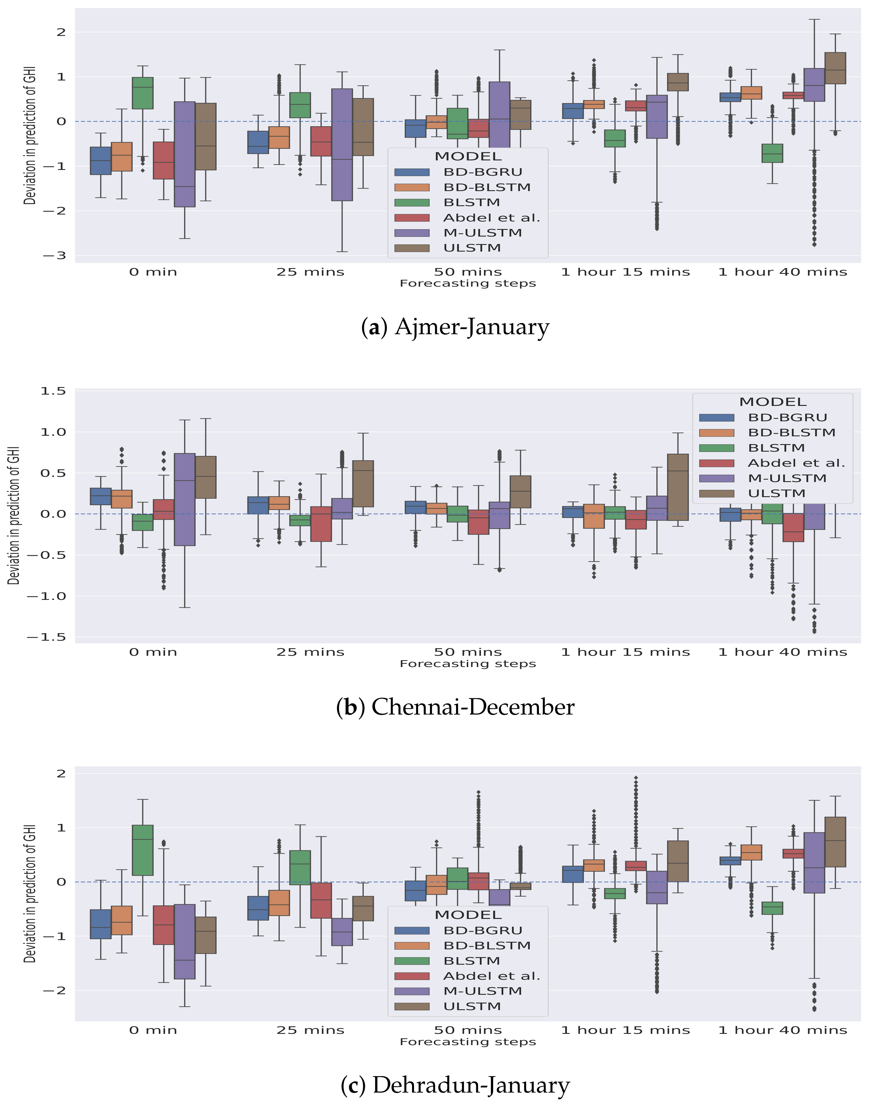
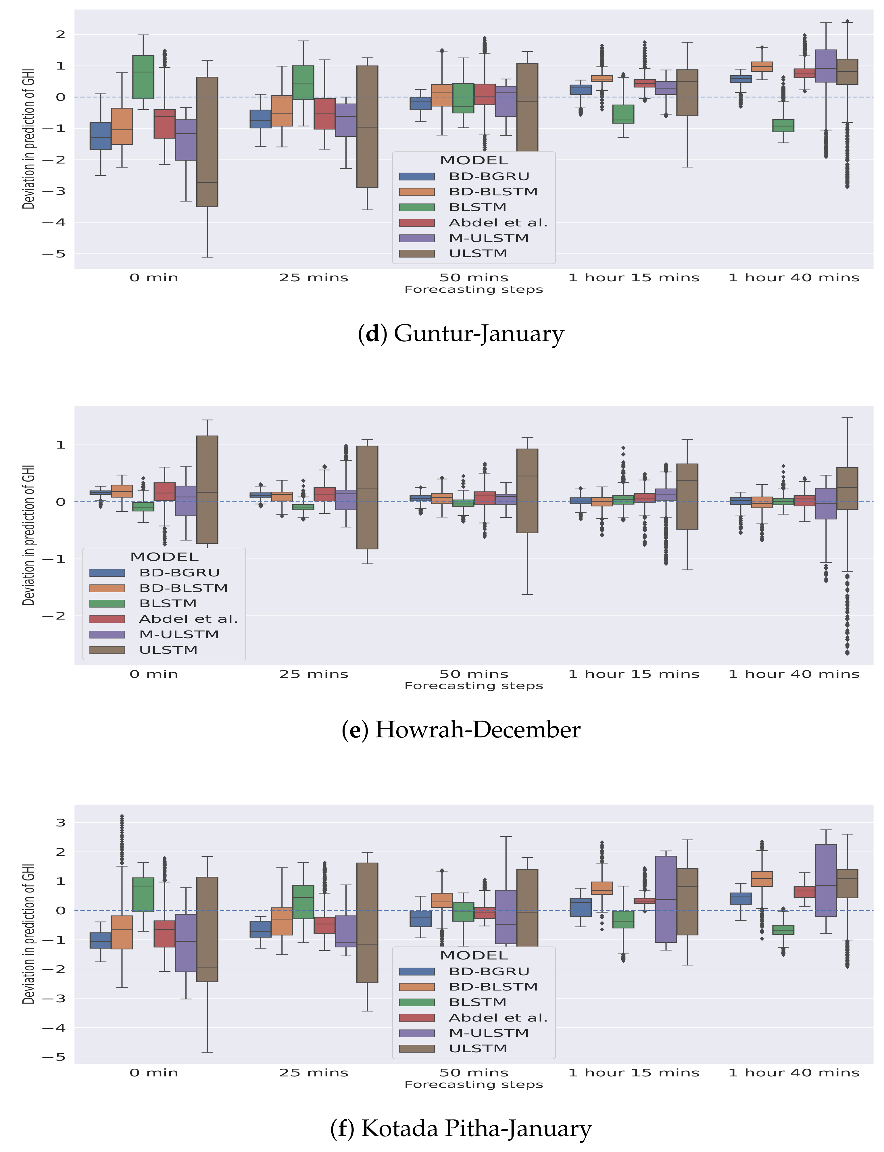
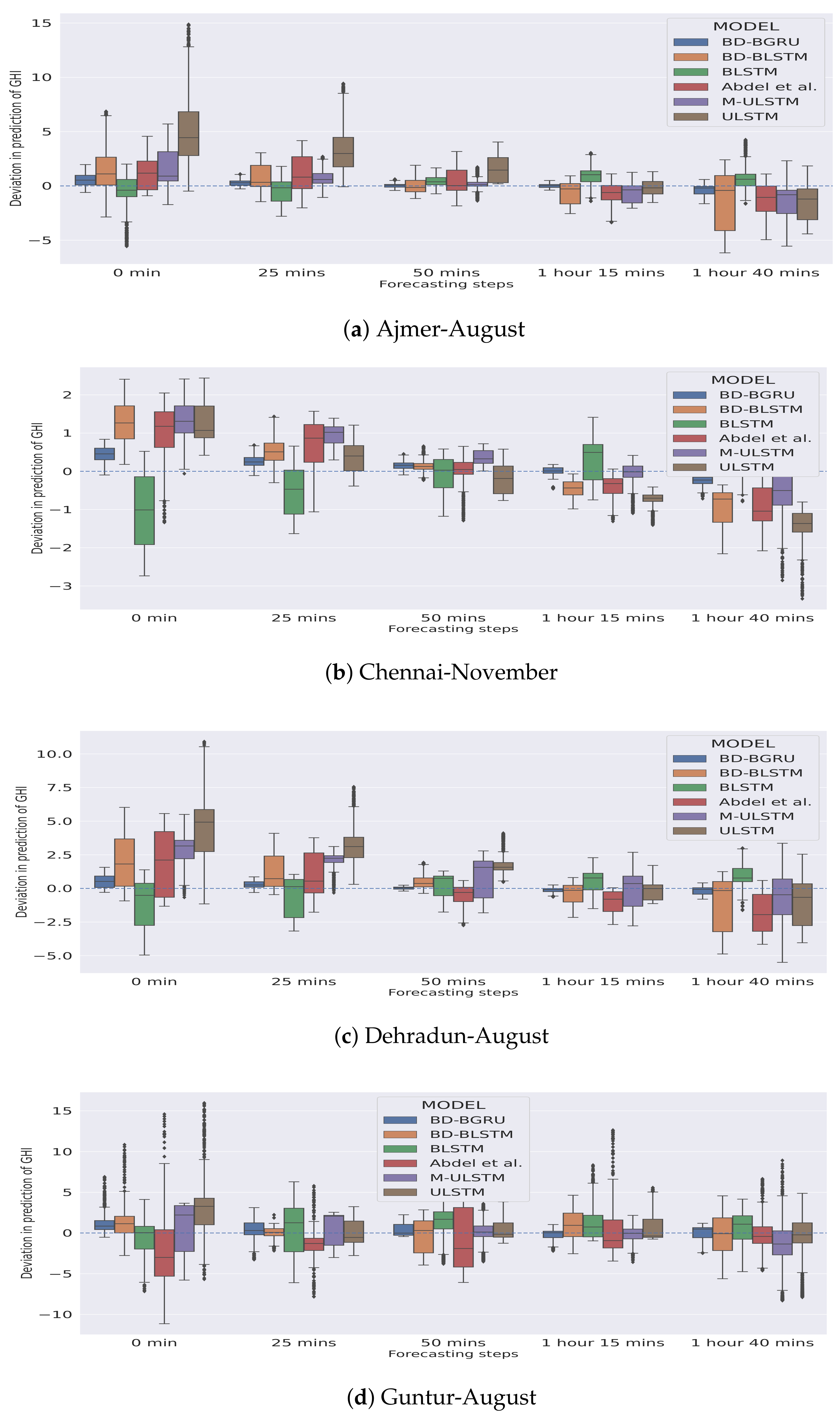
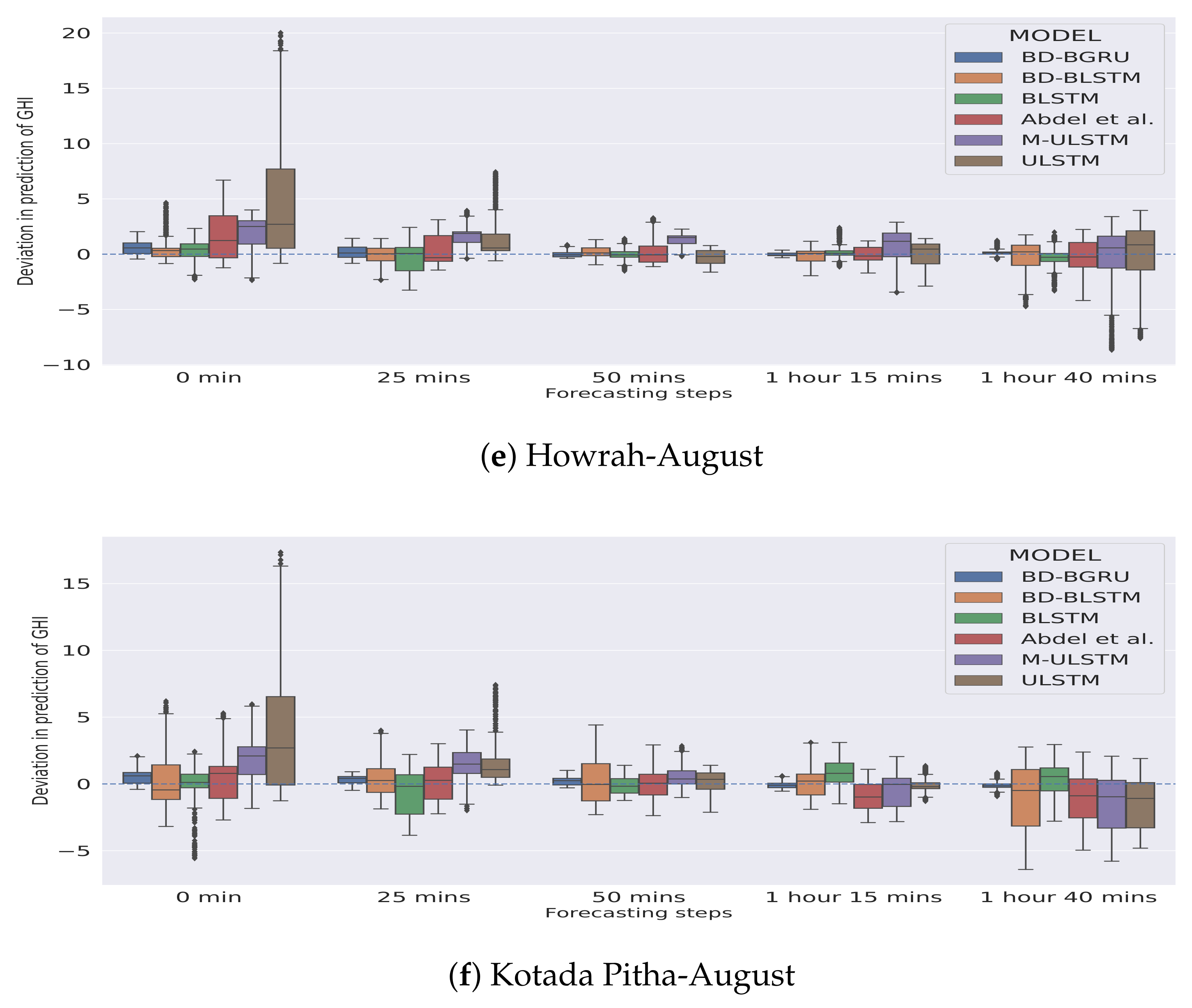
5. Results and Discussions

This section has five subsections. In the first subsection, the prediction performance of M-ULSTM is analyzed compared to ULSTM. After that, in the second subsection, the prediction performance of BLSTM is compared to M-ULSTM. In the third subsection, the forecasting accuracy of BD-BLSTM and BD-BGRU is compared against BLSTM. Then, in the fourth subsection, the overall forecasting performance of BD-BGRU is presented. Finally, in the fifth subsection, the forecasting performance of the proposed model, namely BD-BGRU is compared with some recent works.

5.1. Forecasting Performance of M-ULSTM over ULSTM

In this section, the forecasting performance of M-ULSTM is compared with ULSTM based on nRMSE. In Table 6, the season-specific nRMSE scores for all the stations are presented. The model-specific standard deviation is included in the table to analyze the prediction variability.
Winter: For all the stations, on average M-ULSTM outperformed ULSTM by 83.28%.
Rainy: ULSTM outperformed by M-ULSTM by 38.87%.
Variability: M-ULSTM achieved a much lower standard deviation than ULSTM.

5.2. Forecasting Performance of BLSTM over M-ULSTM

In this section, the overall season specific forecasting performance of BLSTM is compared against M-ULSTM. In Table 7, for all station–season combinations, the forecasting performance is calculated based on nRMSE. The model-specific standard deviation is computed.
Winter: We observed that BLSTM outperformed M-ULSTM by 11.64%.
Rainy: In the rainy season, BLSTM dominated M-ULSTM by 59.53%.
Variability: BLSTM achieved a lower standard deviation in its prediction compared to M-ULSTM.

5.3. Forecasting Performance of BD-BLSTM and BD-BGRU over BLSTM

In Table 8, the forecasting performance of BD-BLSTM and BD-BGRU is compared against BLSTM, where the forecasting accuracy is measured on nRMSE.
  • BD-BLSTM:
    Winter: In the winter season, BD-BLSTM dominated BLSTM by 4.04%.
    Rainy: In the rainy season, BD-BLSTM outperformed BLSTM by 31.81%.
    Variability: BD-BLSTM achieved lower standard deviation compared to BLSTM.
  • BD-BGRU:
    Winter: In the winter season, BD-BGRU outperformed BLSTM by 21.49%.
    Rainy: In the rainy season, BD-BGRU outperformed BLSTM by 53.45%.
    Variability: BD-BGRU achieved a lower standard deviation compared to BLSTM.
Hence, the above experimental result suggested that, when the proposed bidirectional feature representation was used, BD-BLSTM and BD-BGRU can forecast GHI with higher accuracy compared to BLSTM.

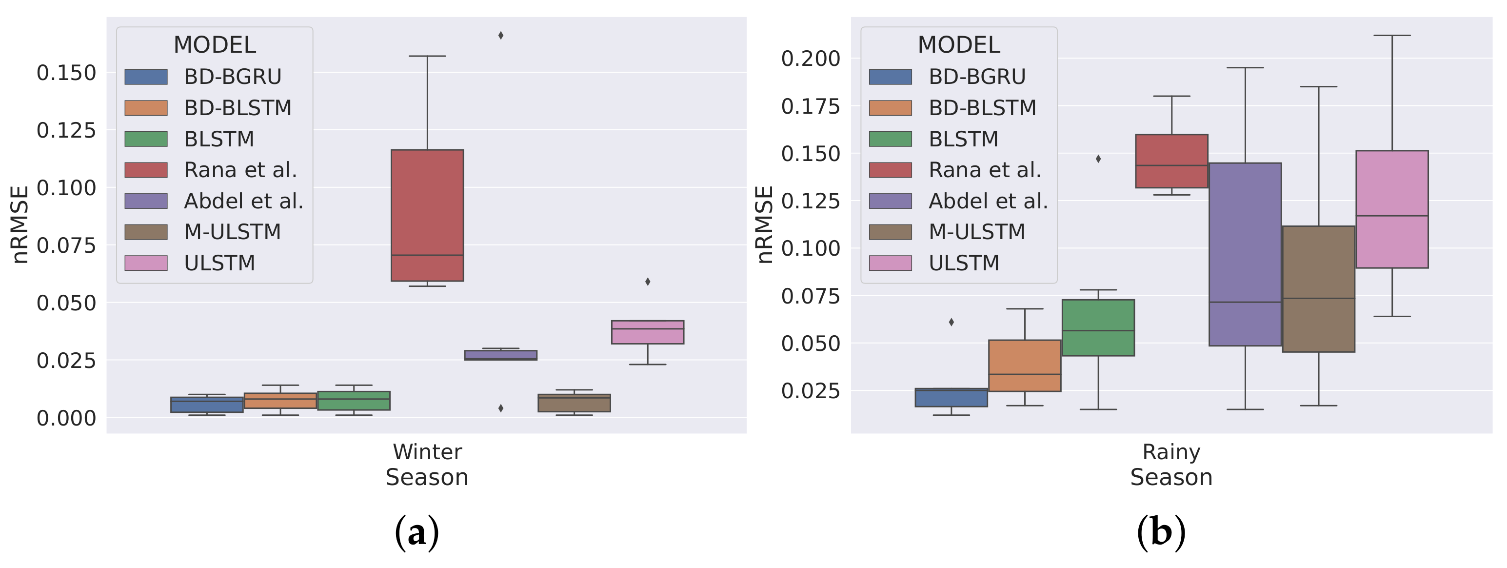
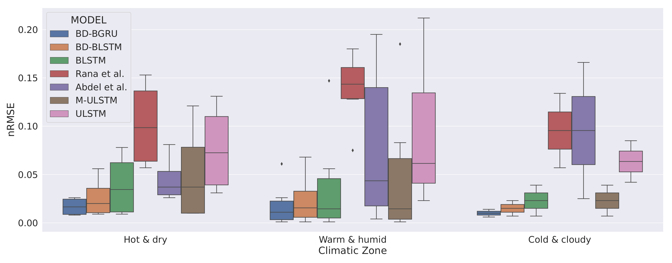
5.4. Overall Forecasting Performance of BD-BGRU

In Figure 5 and Figure 6, the season-specific variability of the deviation of GHI is presented for each station–month combination. The variability was calculated using box-plot and is plotted over different choices of forecasting horizons. The deviation of GHI was calculated by subtracting the predictions from the actual values. We observed that, in winter, for each forecasting horizon, BD-BGRU achieved the lowest variability in the deviation of GHI.
Similarly, in the rainy season, BD-BGRU achieved the lowest variability in its deviation of GHI compared to other models. ULSTM has performed the worst for both winter and rainy seasons. Furthermore, compared to other models for all forecasting horizons, BD-BGRU achieved much lower divergence in its predictions compared to the actual results.

5.5. Comparison with Other Models

In this section, the overall forecasting performance of BD-BGRU is compared against the benchmark models. Table 9 depicts the forecasting performance of BD-BGRU compared to the benchmarks in terms of nRMSE. The summary of this paper is presented in Table 10.
Winter: In winter season, BD-BGRU outperformed [8,29] by 91.17% and 74.93%.
Rainy: In rainy season, [8,29] were outperformed by BD-BGRU by 82.48% and 58.61%. Compared to the benchmark models, BD-BGRU achieved the lowest standard deviation of 0.016.
Figure 7 and Figure 8 depict the season and climatic-zone specific variability in predictions of BD-BGRU and compared with other forecasting models. Figure 7 shows the season-specific box-plot. We observed that, in winter, the variability in predictions of BD-BGRU was the lowest. Moreover, compared to BD-BGRU, BD-BLSTM, BLSTM, and M-ULSTM have similar forecasting performances in winter. However, in the rainy season, the variability in predictions of BD-BGRU is much lower than the other models. Hence, the above discussion suggested that, in winter, BD-BGRU, BD-BLSTM, BLSTM, or M-ULSTM can be alternatively used. However, in the rainy season, BD-BLSTM demonstrated superior forecasting performance.
Figure 8 shows the climatic-zone specific box-plots of the nRMSE scores of all the models. We observed that, in all climatic zones, BD-BGRU achieved the lowest variability in prediction compared to the benchmarks as well as other forecasting models. Moreover, in hot and dry and warm and humid climatic zones, the prediction variability of BD-BGRU is more stable. In all climatic zones, BD-BLSTM is the second best performing forecasting model.
Table 10 depicts the overall summary of this research work. The overall model-specific forecasting accuracy (average nRMSE) is presented individually for each station, and also model-specific standard deviation and mean rank are shown.
  • We observed that BD-BGRU achieved the lowest overall nRMSE score compared to all the other models. In terms of overall forecasting accuracy, BD-BGRU dominated BD-BLSTM by 30.43%.
  • BD-BGRU achieved the lowest standard deviation as 0.016. It implies that in the case of BD-BGRU the variance in predictions of GHI is minimum.
  • BD-BGRU has also achieved the lowest mean rank as 1.16 compared to the other models.

6. Conclusions

In this paper, to forecast inter-day solar irradiation (GHI), five models namely ULSTM, M-ULSTM, BLSTM, BD-BLSTM, and BD-BGRU were implemented. A new feature representation scheme suited for the bidirectional model was proposed. To validate the model, three different climatic zones of India, and two specific seasons, namely the winter and rainy seasons were considered. Each model was implemented for twelve city–month combinations for India. The effectiveness was established through an extensive empirical study over traditional bidirectional models and some recent state-of-the-art models.
M-ULSTM over ULSTM: Individually for each solar station, the forecasting performance of M-ULSTM was compared with ULSTM for both winter and rainy seasons. We observed that, in terms of the nRMSE, for both winter and rainy seasons, M-ULSTM outperformed ULSTM by 83.28% and 38.87%. The standard deviation was lower in the case of M-ULSTM compared to ULSTM. Hence, the above discussion suggests that, compared to ULSTM, the augmented features help M-ULSTM to predict solar irradiation more accurately.
BLSTM over M-ULSTM: We noticed that, overall, for all city–month combinations in the rainy season when the variability of GHI is observed to be higher than winter, BLSTM outperformed M-ULSTM by 59.53%. Hence, the traditional bidirectional LSTM (BLSTM) has forecasted GHI more accurately in the rainy season compared to M-ULSTM.
BD-BGRU and BD-BLSTM over BLSTM: BD-BLSTM and BD-BGRU demonstrated more generalized prediction performance compared to BLSTM. Both BD-BLSTM and BD-BGRU achieved 12.43% and 37.47% lower nRMSE scores compared to BLSTM.
BD-BGRU over BD-BLSTM: In this paper, along with bidirectional LSTM, we also implemented bidirectional GRU, and their forecasting performance was also critically compared. As per the literature, it appears that bidirectional GRU was not used earlier in this domain. The experimental results reveal, for eleven out of twelve city–month combinations, BD-BGRU outperformed BD-BLSTM by 26.67%. Hence, in Indian climatic conditions, BD-BGRU would be the definite choice for intra-day GHI forecasting.
Prediction performance of BD-BLSTM and BD-BGRU over benchmark models: In terms of mean rank, BD-BLSTM and BD-BGRU are the best two methods as compared to the benchmark models. It may be noted that bidirectional GRU may not have been used earlier for prediction in the energy domain.
The limitations of the article are as follows: (1) Including other meteorological parameters, such as temperature, humidity, cloud cover, wind speed, etc., will improve the forecasting accuracy more. However, this study was conducted on one meteorological variable, namely GHI. (2) Currently, one-year data was used at various sites for the proposed algorithm.
As future work, this study can be extended by including more input variables, more years, and including solar stations from other climatic zones.

Author Contributions

Conceptualization, S.M. and S.G.; methodology, S.M.; software, S.M.; validation, S.M., S.G., B.G., A.C., S.S.R., K.B. and A.G.R.; formal analysis, S.M.; investigation, S.M.; resources, S.M.; data curation, S.M., K.B. and A.G.R.; writing—original draft preparation, S.M.; writing—review and editing, S.M., S.G., B.G. and A.C.; visualization, S.M.; supervision, S.G., B.G. and A.C.; project administration, S.G., B.G. and A.C. All authors have read and agreed to the published version of the manuscript.

Funding

Not applicable.

Institutional Review Board Statement

Not applicable.

Informed Consent Statement

Not applicable.

Data Availability Statement

Data is contained within the article.

Acknowledgments

This article resulted from the Indo-USA collaborative project, LISA 2020 between the University of Calcutta, India, and the University of Colorado, USA, and the research is supported by the National Institute of Wind Energy (NIWE) and Technical Education Quality Improvement Programme (TEQIP).

Conflicts of Interest

The authors declare no conflict of interest.

References

  1. Prăvălie, R.; Patriche, C.; Bandoc, G. Spatial assessment of solar energy potential at global scale. A geographical approach. J. Clean. Prod. 2019, 209, 692–721. [Google Scholar] [CrossRef]
  2. Dudley, B. BP statistical review of world energy. BP Stat. Rev. Lond. UK 2018, 6, 00116. [Google Scholar]
  3. Fliess, M.; Join, C.; Voyant, C. Prediction bands for solar energy: New short-term time series forecasting techniques. Sol. Energy 2018, 166, 519–528. [Google Scholar] [CrossRef] [Green Version]
  4. Pan, C.; Tan, J.; Feng, D. Prediction intervals estimation of solar generation based on gated recurrent unit and kernel density estimation. Neurocomputing 2020, 453, 552–562. [Google Scholar] [CrossRef]
  5. Alzahrani, A.; Shamsi, P.; Dagli, C.; Ferdowsi, M. Solar irradiance forecasting using deep neural networks. Procedia Comput. Sci. 2017, 114, 304–313. [Google Scholar] [CrossRef]
  6. Hejase, H.A.; Al-Shamisi, M.H.; Assi, A.H. Modeling of global horizontal irradiance in the United Arab Emirates with artificial neural networks. Energy 2014, 77, 542–552. [Google Scholar] [CrossRef]
  7. Lai, C.S.; Zhong, C.; Pan, K.; Ng, W.W.; Lai, L.L. A deep learning based hybrid method for hourly solar radiation forecasting. Expert Syst. Appl. 2021, 177, 114941. [Google Scholar] [CrossRef]
  8. Abdel-Nasser, M.; Mahmoud, K. Accurate photovoltaic power forecasting models using deep LSTM-RNN. Neural Comput. Appl. 2019, 31, 2727–2740. [Google Scholar] [CrossRef]
  9. Qing, X.; Niu, Y. Hourly day-ahead solar irradiance prediction using weather forecasts by LSTM. Energy 2018, 148, 461–468. [Google Scholar] [CrossRef]
  10. Alfadda, A.; Rahman, S.; Pipattanasomporn, M. Solar irradiance forecast using aerosols measurements: A data driven approach. Sol. Energy 2018, 170, 924–939. [Google Scholar] [CrossRef]
  11. Srivastava, S.; Lessmann, S. A comparative study of LSTM neural networks in forecasting day-ahead global horizontal irradiance with satellite data. Sol. Energy 2018, 162, 232–247. [Google Scholar] [CrossRef]
  12. Cannizzaro, D.; Aliberti, A.; Bottaccioli, L.; Macii, E.; Acquaviva, A.; Patti, E. Solar radiation forecasting based on convolutional neural network and ensemble learning. Expert Syst. Appl. 2021, 181, 115167. [Google Scholar] [CrossRef]
  13. Perez, R.; Lorenz, E.; Pelland, S.; Beauharnois, M.; Van Knowe, G.; Hemker, K., Jr.; Heinemann, D.; Remund, J.; Müller, S.C.; Traunmüller, W.; et al. Comparison of numerical weather prediction solar irradiance forecasts in the US, Canada and Europe. Sol. Energy 2013, 94, 305–326. [Google Scholar] [CrossRef]
  14. Voyant, C.; Notton, G.; Kalogirou, S.; Nivet, M.L.; Paoli, C.; Motte, F.; Fouilloy, A. Machine learning methods for solar radiation forecasting: A review. Renew. Energy 2017, 105, 569–582. [Google Scholar] [CrossRef]
  15. Mellit, A.; Mekki, H.; Messai, A.; Kalogirou, S.A. FPGA-based implementation of intelligent predictor for global solar irradiation, Part I: Theory and simulation. Expert Syst. Appl. 2011, 38, 2668–2685. [Google Scholar] [CrossRef]
  16. Kumari, P.; Toshniwal, D. Extreme gradient boosting and deep neural network based ensemble learning approach to forecast hourly solar irradiance. J. Clean. Prod. 2021, 279, 123285. [Google Scholar] [CrossRef]
  17. Wan, H.; Guo, S.; Yin, K.; Liang, X.; Lin, Y. CTS-LSTM: LSTM-based neural networks for correlatedtime series prediction. Knowl.-Based Syst. 2020, 191, 105239. [Google Scholar] [CrossRef]
  18. Li, Y.; Zhu, Z.; Kong, D.; Han, H.; Zhao, Y. EA-LSTM: Evolutionary attention-based LSTM for time series prediction. Knowl.-Based Syst. 2019, 181, 104785. [Google Scholar] [CrossRef] [Green Version]
  19. Wang, H.; Yang, Z.; Yu, Q.; Hong, T.; Lin, X. Online reliability time series prediction via convolutional neural network and long short term memory for service-oriented systems. Knowl.-Based Syst. 2018, 159, 132–147. [Google Scholar] [CrossRef]
  20. Long, W.; Lu, Z.; Cui, L. Deep learning-based feature engineering for stock price movement prediction. Knowl.-Based Syst. 2019, 164, 163–173. [Google Scholar] [CrossRef]
  21. Iwana, B.K.; Frinken, V.; Uchida, S. DTW-NN: A novel neural network for time series recognition using dynamic alignment between inputs and weights. Knowl.-Based Syst. 2020, 188, 104971. [Google Scholar] [CrossRef]
  22. LeCun, Y.; Bengio, Y.; Hinton, G. Deep learning. Nature 2015, 521, 436–444. [Google Scholar] [CrossRef] [PubMed]
  23. Aslam, M.; Lee, J.M.; Kim, H.S.; Lee, S.J.; Hong, S. Deep Learning Models for Long-Term Solar Radiation Forecasting Considering Microgrid Installation: A Comparative Study. Energies 2019, 13, 147. [Google Scholar] [CrossRef] [Green Version]
  24. Mukherjee, A.; Ain, A.; Dasgupta, P. Solar Irradiance Prediction from Historical Trends Using Deep Neural Networks. In Proceedings of the 2018 IEEE International Conference on Smart Energy Grid Engineering (SEGE), Oshawa, ON, Canada, 12–15 August 2018; pp. 356–361. [Google Scholar] [CrossRef]
  25. Castangia, M.; Aliberti, A.; Bottaccioli, L.; Macii, E.; Patti, E. A compound of feature selection techniques to improve solar radiation forecasting. Expert Syst. Appl. 2021, 178, 114979. [Google Scholar] [CrossRef]
  26. Feng, C.; Zhang, J. SolarNet: A sky image-based deep convolutional neural network for intra-hour solar forecasting. Sol. Energy 2020, 204, 71–78. [Google Scholar] [CrossRef]
  27. Sharadga, H.; Hajimirza, S.; Balog, R.S. Time series forecasting of solar power generation for large-scale photovoltaic plants. Renew. Energy 2019. [Google Scholar] [CrossRef]
  28. Zheng, J.; Zhang, H.; Dai, Y.; Wang, B.; Zheng, T.; Liao, Q.; Liang, Y.; Zhang, F.; Song, X. Time series prediction for output of multi-region solar power plants. Appl. Energy 2020, 257, 114001. [Google Scholar] [CrossRef]
  29. Rana, M.; Rahman, A. Multiple steps ahead solar photovoltaic power forecasting based on univariate machine-learning models and data re-sampling. Sustain. Energy Grids Netw. 2020, 21, 100286. [Google Scholar] [CrossRef]
  30. Benali, L.; Notton, G.; Fouilloy, A.; Voyant, C.; Dizene, R. Solar radiation forecasting using artificial neural network and random forest methods: Application to normal beam, horizontal diffuse and global components. Renew. Energy 2019, 132, 871–884. [Google Scholar] [CrossRef]
  31. Yang, Z.; Mourshed, M.; Liu, K.; Xu, X.; Feng, S. A novel competitive swarm optimized RBF neural network model for short-term solar power generation forecasting. Neurocomputing 2020, 397, 415–421. [Google Scholar] [CrossRef]
  32. Torres-Barrán, A.; Alonso, Á.; Dorronsoro, J.R. Regression tree ensembles for wind energy and solar radiation prediction. Neurocomputing 2019, 326, 151–160. [Google Scholar] [CrossRef]
  33. Wang, K.; Qi, X.; Liu, H. Photovoltaic power forecasting based LSTM-Convolutional Network. Energy 2019, 189, 116225. [Google Scholar] [CrossRef]
  34. Malakar, S.; Goswami, S.; Ganguli, B.; Chakrabarti, A.; Roy, S.S.; Boopathi, K.; Rangaraj, A. Designing a long short-term network for short-term forecasting of global horizontal irradiance. SN Appl. Sci. 2021, 3, 477. [Google Scholar] [CrossRef]
  35. Wang, K.; Li, K.; Zhou, L.; Hu, Y.; Cheng, Z.; Liu, J.; Chen, C. Multiple convolutional neural networks for multivariate time series prediction. Neurocomputing 2019, 360, 107–119. [Google Scholar] [CrossRef]
  36. Ghimire, S.; Deo, R.C.; Raj, N.; Mi, J. Deep solar radiation forecasting with convolutional neural network and long short-term memory network algorithms. Appl. Energy 2019, 253, 113541. [Google Scholar] [CrossRef]
  37. Hochreiter, S.; Schmidhuber, J. Long short-term memory. Neural Comput. 1997, 9, 1735–1780. [Google Scholar] [CrossRef] [PubMed]
  38. Hochreiter, S. The vanishing gradient problem during learning recurrent neural nets and problem solutions. Int. J. Uncertain. Fuzziness Knowl. Based Syst. 1998, 6, 107–116. [Google Scholar] [CrossRef] [Green Version]
  39. Pascanu, R.; Mikolov, T.; Bengio, Y. Understanding the exploding gradient problem. arXiv 2012, arXiv:1211.5063. [Google Scholar]
  40. Chung, J.; Gulcehre, C.; Cho, K.; Bengio, Y. Empirical evaluation of gated recurrent neural networks on sequence modeling. arXiv 2014, arXiv:1412.3555. [Google Scholar]
  41. Cho, K.; Van Merriënboer, B.; Bahdanau, D.; Bengio, Y. On the properties of neural machine translation: Encoder-decoder approaches. arXiv 2014, arXiv:1409.1259. [Google Scholar]
  42. Wichrowska, O.; Maheswaranathan, N.; Hoffman, M.W.; Colmenarejo, S.G.; Denil, M.; Freitas, N.; Sohl-Dickstein, J. Learned optimizers that scale and generalize. In Proceedings of the International Conference on Machine Learning, Sydney, Australia, 6–11 August 2017; pp. 3751–3760. [Google Scholar]
  43. Zhang, Z. Improved adam optimizer for deep neural networks. In Proceedings of the 2018 IEEE/ACM 26th International Symposium on Quality of Service (IWQoS), Banff, AB, Canada, 4–6 June 2018; pp. 1–2. [Google Scholar]
  44. Bottou, L. Stochastic gradient descent tricks. In Neural Networks: Tricks of the Trade; Springer: Berlin/Heidelberg, Germany, 2012; pp. 421–436. [Google Scholar]
  45. Graves, A.; Schmidhuber, J. Framewise phoneme classification with bidirectional LSTM and other neural network architectures. Neural Netw. 2005, 18, 602–610. [Google Scholar] [CrossRef]
  46. Graves, A.; Mohamed, A.R.; Hinton, G. Speech recognition with deep recurrent neural networks. In Proceedings of the 2013 IEEE International Conference on Acoustics, Speech and Signal Processing, Vancouver, BC, Canada, 26–31 May 2013; pp. 6645–6649. [Google Scholar] [CrossRef] [Green Version]
  47. Iqbal, M. An Introduction to Solar Radiation; Elsevier: Amsterdam, The Netherlands, 2012. [Google Scholar]
  48. Géron, A. Hands-On Machine Learning with Scikit-Learn, Keras, and TensorFlow: Concepts, Tools, and Techniques to Build Intelligent Systems; O’Reilly Media: Newton, MA, USA, 2019. [Google Scholar]
  49. Wazwaz, A.M. The tanh method for traveling wave solutions of nonlinear equations. Appl. Math. Comput. 2004, 154, 713–723. [Google Scholar] [CrossRef]
  50. Kingma, D.P.; Ba, J. Adam: A method for stochastic optimization. arXiv 2014, arXiv:1412.6980. [Google Scholar]
  51. Yoo, Y. Hyperparameter optimization of deep neural network using univariate dynamic encoding algorithm for searches. Knowl.-Based Syst. 2019, 178, 74–83. [Google Scholar] [CrossRef]
  52. Snoek, J.; Larochelle, H.; Adams, R.P. Practical Bayesian Optimization of Machine Learning Algorithms. Advances in Neural Information Processing Systems. 2012, pp. 2951–2959. Available online: https://proceedings.neurips.cc/paper/2012/file/05311655a15b75fab86956663e1819cd-Paper.pdf (accessed on 20 November 2021).
  53. Bergstra, J.S.; Bardenet, R.; Bengio, Y.; Kégl, B. Algorithms for Hyper-Parameter Optimization. Advances in Neural Information Processing Systems. 2011, pp. 2546–2554. Available online: https://hal.inria.fr/hal-00642998 (accessed on 20 November 2021).
  54. Bergstra, J.; Yamins, D.; Cox, D.D. Hyperopt: A python library for optimizing the hyperparameters of machine learning algorithms. In Proceedings of the 12th Python in Science Conference; Citeseer: University Park, PA, USA, 2013; pp. 13–20. [Google Scholar]
  55. Pedregosa, F.; Varoquaux, G.; Gramfort, A.; Michel, V.; Thirion, B.; Grisel, O.; Blondel, M.; Prettenhofer, P.; Weiss, R.; Dubourg, V.; et al. Scikit-learn: Machine learning in Python. J. Mach. Learn. Res. 2011, 12, 2825–2830. [Google Scholar]
  56. Bergstra, J.; Bengio, Y. Random search for hyper-parameter optimization. J. Mach. Learn. Res. 2012, 13, 281–305. [Google Scholar]
Figure 1. A neural network based on GRU cells.
Make 03 00047 g001
Figure 2. A network of bidirectional GRU (a) contexts with similar lengths and (b) contexts with different length.
Make 03 00047 g002
Figure 4. Solar stations based on climatic zones.
Make 03 00047 g004
Figure 5. Variability in deviation of GHI (W/m 2 ) in the winter season.
Make 03 00047 g005aMake 03 00047 g005b
Figure 6. Variability in deviation of GHI (W/m 2 ) in the rainy season.
Make 03 00047 g006aMake 03 00047 g006b
Figure 7. Season specific variability in predictions.
Make 03 00047 g007
Figure 8. Climatic-zone specific variability in predictions.
Make 03 00047 g008
Table 1. Studies based on currently implemented models on solar irradiation prediction.
CitationDataModel NameForecastingWindowCountryCorrectnessA/D
[8]Time SeriesLSTM (Unidirectional)HourlyEgyptThe claimed forecasting error is 82.15, and 136.87 in terms of RMSEPerfromed better compared to MLR, BRT, and NN
[27]Time SeriesBi-LSTM (Bidirectional)HourlyChinaBI-LSTM produced correlation coefficient of 98%, and RMSE of 0.791Same past context used for both the forward and the backward mode
[28]Time SeriesPSO-LSTM(Bidirectional)Multiple daysChinaPSO-LSTM achieved the lowest MAE, and RMSE as 8.14, and 19.41Same past context used for both the forward and the backward mode
[36]Time SeriesCNN-LSTM(Unidirectional)1-Day, 1-Week, 2-Week and 1-MonthAustraliaIt achieved lower MAPE < 11%, and RRMSE < 15% compared to benchmark modelsThis study islimited to one solar station
[33]Time SeriesLSTM-CNN (Unidirectional)Multiple daysChinaLSTM-CNN achieved the best MAE, RMSE, and MAPE as 0.221, 0.621, and 0.042This study islimited to onesolar station
[6]Time SeriesMLP (Unidirectional)MonthlyUAEMLP has shown the best MBE, ans RMSE as 0.0003, and 0.179The model is validated for three solar stations
[30]Time SeriesRF1 h to 6 hFranceRF achieved the lowest forecasting error as 19.65% to 27.78% in terms of RMSEThis study is restricted to one solar station
[10]Aerosol Optical Depth (AOD) and the Angstrom Exponent dataMLP (Unidirectional)1 hSaudi ArabiaMLP achieved lower RMSE under 4% and forecast skill of over 42%The study is restricted to one solar site
[29]Time SeriesRF5 min to 3 hAustraliaRF achieved the lowest overall MAE, and MRE as 110.46, and 10.5%The proposed model is univariate, and restricted to one solar site
Table 3. Description of the data.
City with MonthLongitudeLatitudeStandard DeviationClimatic Zone
Ajmer (January) 74 . 66 E 26 . 40 N47.64Hot and dry
Chennai (December) 80 . 22 E 12 . 96 N48.26Warm and humid
Dehradun (January) 77 . 97 E 30 . 42 N46.94Cold and cloudy
Guntur (January) 80 . 53 E 16 . 37 N49.46Warm and humid
Howrah (December) 88 . 31 E 22 . 55 N45.16Warm and humid
Kotada Pitha (January) 71 . 21 E 21 . 95 N48.55Hot and dry
Ajmer (August) 74 . 66 E 26 . 40 N78.33Hot and dry
Chennai (November) 80 . 22 E 12 . 96 N51.88Warm and humid
Dehradun (August) 77 . 97 E 30 . 42 N74.78Cold and cloudy
Guntur (August) 80 . 53 E 16 . 37 N90.36Warm and humid
Howrah (August) 88 . 31 E 22 . 55 N80.22Warm and humid
Kotada Pitha (August) 80 . 53 E 16 . 37 N82.91Hot and dry
Table 4. Hyper-parameters to optimize.
ModelsHyper-ParametersValues
Number of hidden layers1, 2, 3
Nodes in hidden layer25, 50, 100
BLSTM/BD-BLSTM/BD-BGRU/ULSTM/M-ULSTMLearning rate0.1, 0.01, 0.001
Batch size1, 10, 20, 50, 100
Epoch20, 40, 60, 60, 80, 100
Table 5. Architectural similarity and dissimilarity of the proposed model compared to the reference models.
Model Attributes[29][8]BD-BLSTM/BD-BGRU *
Similarities
Domain:Solar predictionSolar predictionSolar prediction
Input data:Time seriesTime seriesTime series
Prediction type:Uni-variateUni-variateUni-variate
Series type:Non-stationaryNon-stationaryNon-stationary
Dissimilarities
Model type:Random ForestNeural NetworkNeural Network
Sequential model:×
Memory:×
Stateful:××
Activation:×Defaulttanh
Bidirectional:××
Bidirectional feature:××
Stateful:××
Table 6. The forecasting performance of M-ULSTM and ULSTM measured on nRMSE.
AjmerChennaiDehradunGunturHowrahKotada Pitha σ
ModelsWinterRainyWinterRainyWinterRainyWinterRainyWinterRainyWinterRainy
ULSTM0.0420.1030.0350.0640.0420.0560.0590.2120.0230.1580.0310.1310.0581
M-ULSTM *0.0100.0640.0010.0170.0070.0390.0120.1850.0010.0830.0100.1210.038
Table 7. The forecasting performance of BLSTM and M-ULSTM measured on nRMSE.
AjmerChennaiDehradunGunturHowrahKotada Pitha σ
ModelsWinterRainyWinterRainyWinterRainyWinterRainyWinterRainyWinterRainy
M-ULSTM0.0100.0640.0010.0170.0070.0390.0120.0180.0010.0830.0100.1210.038
BLSTM *0.0090.0570.0020.0150.0070.0390.0140.1470.0010.0560.0120.0780.025
Table 8. The forecasting performance of BLSTM, BD-BLSTM, and BD-BGRU measured on nRMSE.
AjmerChennaiDehradunGunturHowrahKotada Pitha σ
ModelsWinterRainyWinterRainyWinterRainyWinterRainyWinterRainyWinterRainy
BLSTM0.0090.0570.0020.0150.0070.0390.0140.1470.0010.0560.0120.0780.025
BD-BLSTM0.0090.00290.0030.00170.0070.0230.0140.0680.0010.0380.0110.0560.021
BD-BGRU *0.0080.0240.0010.0120.0060.0140.0100.0610.0010.0260.0090.0260.016
Table 9. The forecasting performance of BD-BGRU compared to the benchmark models.
AjmerChennaiDehradunGunturHowrahKotada Pitha σ
ModelsWinterRainyWinterRainyWinterRainyWinterRainyWinterRainyWinterRainy
[29]0.0570.1310.1300.1280.0570.1340.0750.1800.1570.1620.0660.1530.043
[8]0.0260.0440.1660.0150.0250.1660.0250.1950.0040.0620.0300.0810.067
BD-BGRU *0.0080.0240.0010.0120.0060.0140.0100.0610.0010.0260.0090.0260.016
Table 10. Overall performance summary of the forecasting models.
ModelsOverall nRMSEStandard Deviation ( σ ) Mean Rank
[29]0.1190.0436.58
[8]0.0690.0674.87
ULSTM0.0820.0585.91
M-ULSTM0.0450.0383.58
BLSTM0.0360.0253.12
BD-BLSTM0.0230.0212.75
BD-BGRU *0.0160.0161.16
Publisher’s Note: MDPI stays neutral with regard to jurisdictional claims in published maps and institutional affiliations.

