Analysis of Explainers of Black Box Deep Neural Networks for Computer Vision: A Survey

Abstract

Deep Learning is a state-of-the-art technique to make inference on extensive or complex data. As a black box model due to their multilayer nonlinear structure, Deep Neural Networks are often criticized as being non-transparent and their predictions not traceable by humans. Furthermore, the models learn from artificially generated datasets, which often do not reflect reality. By basing decision-making algorithms on Deep Neural Networks, prejudice and unfairness may be promoted unknowingly due to a lack of transparency. Hence, several so-called explanators, or explainers, have been developed. Explainers try to give insight into the inner structure of machine learning black boxes by analyzing the connection between the input and output. In this survey, we present the mechanisms and properties of explaining systems for Deep Neural Networks for Computer Vision tasks. We give a comprehensive overview about the taxonomy of related studies and compare several survey papers that deal with explainability in general. We work out the drawbacks and gaps and summarize further research ideas.

1. Introduction

Artificial Intelligence (AI)-based technologies are increasingly being used to make inference on classification or regression problems: automated image and text interpretation in medicine, insurance, advertisement, public video surveillance, job applications, or credit scoring save staff and time and are successful in practice. The severe drawback is that many of these technologies are black boxes and the referenced results can hardly be understood by the user. Quality assurance and the measurability of safety and reliability of explainers has not been sufficiently researched, yet. Das and Rad [1] advised against blindly trusting the results of a highly predictive classifier, by today’s standard, due to the strong influence of data bias, trustability, and adversarial examples in Machine Learning (ML). These findings are being observed more and more, and consequently, explainable ML is now applied to some questions, for example to explore COVID-19 [2,3,4].

1.1. Motivation: Ethical Questions

Recent models are more complex, and Deep-Learning (DL) architectures are becoming deeper and deeper, comprising millions of parameters. Following this, the classification process is merely comprehensible by humans. Metrics such as accuracy or the mean average precision depend on the quality of hand-annotated data. However, these metrics are often the only values that evaluate the learning algorithm itself.

In recent years, several weaknesses of Deep-Learning models were found (even high-performing models are affected). For instance, object detectors can be fooled easily by applying small changes to input images or by creating artificial adversarial examples [5,6]. Such attacks could reveal that supposedly good models are not robust or focus on less relevant features for classifying objects; see the examples in the following. The problem is that the neural network learns only from the training data, which should characterize the task. However, suitable training data are tedious to create and annotate; hence, they are not always perfect. If in the training data there is a bias, the models will learn it as well. Now, exemplary attacks on neural networks are presented:

A dog or wolf classifier turned out to be just a good snow detector [7] because of a bias in the background of the training images. The reason was that most of the photos for the training set of wolfs were taken on days with snowy weather, while the dog images were shot in landscapes without snow. There are several cases that underline the negative characteristics of a DNN: changing only one pixel in an input image or one letter in a sentence or even adding small-magnitude perturbations could change the prediction [8,9,10]; see also Figure 1 (we have obtained the necessary copyright permission to reprint this and all other figures in this work). Adversarial examples with serious impact exist; stickers fixed on road signs [11] or extended adversarial patch attacks in optical flow networks [12] could lead to dangerous misinterpretation. Glasses confuse face detectors by imitating persons [13,14]. Additional examples are depicted in Figure 2, Figure 3 and Figure 4. All these cases show how harmful it could be to rely on a black box with supposedly good performance results without quality control. However, currently applied DNN methods and models are such vulnerable black boxes.

Since the European Union’s new General Data Protection Regulation (GDPR) was passed in the EU in May 2018, it has restricted the use of Machine Learning and automated individual decision-making and focuses on the protection of sensitive data of persons such as their age, sex, ancestry, name, or place of residence, for instance. The GDPR also imposes a data quality requirement in the AI area because the quality of the training datasets is decisive for the outcome. If a result affects users, they should be able to demand for explanations of the model’s decision that was made about them [15]. The explanation has to be transmitted in a precise, transparent, understandable, and easily accessible form and in a clear and simple language. For example, if a doctor makes a mistake, the patient wants to know why. Was the mistake excusable, or does the mistake reflect negligence, even intentionally or occurring due to other factors?

Similarly, if a model fails and contributes to an adverse clinical event or malpractice, doctors need to be able to understand why it produced the result and how it reached a decision. Reference [16] proposed ten commandments as practical guidelines in his work about ethical medical AI.

Individual human’s decisions are not free from prejudice, but it should be ensured that a model for a selection procedure, e.g., for job proposals or suspended sentences, should not discriminate humans in general because of sex, origin, etc. Here, disadvantages can arise for individuals, groups of persons, or a whole society. The prevailing conditions can thereby deteriorate more and more, for instance, due to a gender word bias [17]. An interesting example is word embeddings [18] that a Natural Language Processing (NLP) algorithm creates from training datasets, which are just any available texts of a specific origin [19]. The discrimination of women, the disabled, black people, etc., seem to be deeply anchored in these texts because of authors’ general or specific prejudices with the serious consequence that the model learns that to be real. This could reinforce discrimination and unfairness. Implicit Association Tests [20] have uncovered stereotype biases, which people are not aware of. If the model supposes—and studies [18,21,22] show—that doctors are male and nurses are female, furthermore, that women are sensitive and men are successful, it will sort out all women who apply as a chief doctor—only because of their sex—no need to check their qualification. If in the training data, foreigners have predominantly less income and increased unemployment, an automatic credit scoring model will suggest a higher interest rate or even refuse the request only because of the origin and without considering the individual financial situation. In summary, this means models that are trained on contaminated data may spread prejudices and discrimination and unfairness is able to progress.

Figure 2. Reference [23] created artificial images that were unrecognizable by humans, but the state-of-the-art classifier was very confident that they were known objects. Images are either directly (top) or indirectly (bottom) encoded.

Figure 2. Reference [23] created artificial images that were unrecognizable by humans, but the state-of-the-art classifier was very confident that they were known objects. Images are either directly (top) or indirectly (bottom) encoded.

Figure 3. Texture–shape cue conflict [24]: texture (left) is classified as elephant; content (middle) is classified as cat; texture–shape (right) is classified as elephant because of a texture bias.

Figure 3. Texture–shape cue conflict [24]: texture (left) is classified as elephant; content (middle) is classified as cat; texture–shape (right) is classified as elephant because of a texture bias.

Figure 4. Reference [24] showed that Convolutional Neural Networks focus more on texture than on shapes and that it is a good idea to improve shape bias to obtain more reliable results in the way humans would interpret the content of an image.

Figure 4. Reference [24] showed that Convolutional Neural Networks focus more on texture than on shapes and that it is a good idea to improve shape bias to obtain more reliable results in the way humans would interpret the content of an image.

1.2. Contribution

Gaining understanding of and insight into the models should uncover the named problems. Properties of a model such as transparency and interpretability are basic to build provider trust and fairness. If this succeeds, the causes of the discrimination and serious mistakes can be prevented, additionally. There is the opportunity to improve society by making automated decisions free of prejudice. Our contribution on the way of achieving this goal is to give an overview of state-of-the-art-explainers with regard to their taxonomy by differentiating their mechanisms and technical properties. We did not limit our work to explaining methods, but also looked at the meaning of understanding a machine in general. To our knowledge, this is the first survey paper that focuses mainly on ML black box DNNs for Computer Vision tasks, but also summarizing some other related ML areas.

2. Overview of Explaining Systems for DNNs

We give a short introduction to the early approaches to explain the inner operations of Machine Learning. After that we, focus on understanding DNNs.

2.1. Early Machine Learning Explaining Systems

Early explaining systems for ML black boxes go back to 1986 with Generalized Additive Models (GAM) [25]. GAMs are global statistic models that use smooth functions, which are estimated using a scatterplot smoother. The technique is applicable to any likelihood-based regression model, provides a flexible method for identifying nonlinear covariate effects in exponential family models and other likelihood-based regression models, and has the advantage of being completely automatic. In its most general form, the algorithm can be applied to any situation in which a criterion is optimized involving one or more smooth functions. Later, Decision Trees were shown to be successful classification tools that provide individual explanations [26,27]. A Decision Tree is a tree-like graph of decisions and their possible consequences, which visualizes an algorithm that only contains condition control statements. Classification begins with the application of the root node test, its outcome determining the branch to a succeeding node, whereby interior nodes are tests applied to instances during classification and branches from an interior node correspond to the possible test outcomes. The process is recursively applied until a leaf node is reached. Finally, the instance is labeled with the class of the leaf node [28]. Another approach [29] shows the marginal effect of one or two features on the prediction of learning techniques using Partial Dependence Plots (PDPs). The method gives a statement about the global relationship of a feature and whether its relation to the outcome is linear, monotonic, or more complex. The PDP is the average of Individual Conditional Expectation (ICE) over all features. ICE [30] points to how the prediction changes if a feature changes. The PDP is limited to two features. Another example is the early use of Explainable AI (XAI) [31] in a simulator game for the commercial platform training aid Full Spectrum Command (FSC) developed by the USC Institute for Creative Technologies and Quicksilver Software, Inc., for the U.S. Army, designed not for entertainment, but as a training tool to achieve a targeted training objective. FSC includes an XAI system that allows the user to ask any subordinate soldier questions about the current behavior of the platoon during the after-action review phase of the game. In addition to this, XAI identifies key events to be highlighted in the after-action review. It was motivated by previous work such as [32], a rule-based expert system that uses early AI techniques and a model of the interaction between physicians and human consultants to attempt to satisfy the demands of a user community.

The proposed procedure of [33] is based on a set of assumptions, which allows one to explain why the model predicted a particular label for a single instance and what features were most influential for that particular instance for several classification models using Decision Trees. The framework provides local explanation vectors as class probability gradients, which yield the relevant features of every point of interest in the data space. For models where such gradient information cannot be calculated explicitly, the authors employed a probabilistic approximate mimic of the model to be explained.

We do not comment further on early studies of explaining systems of Random Forests [34], Naive Bayesian classifiers [35,36,37], Support Vector Machines (SVMs) [38,39], or other early Machine Learning prediction methods [40].

2.2. Methods and Properties of DNN Explainers

In the last few years, the importance of DNNs in inference tasks grew rapidly, and with the increasing complexity of these models, the need for better explanations did as well. The most commonly used DNNs for image or video processing [41,42,43] are Convolutional Neural Networks (CNNs) [44], for videos [43] or sequences of text Recurrent Neural Networks (RNNs) [45], and especially for language modeling [46] Long Short-Term Memory networks (LSTMs) [47]. There exist some general surveys of methods for explaining several machine learning black boxes, so-called XAI, that cover a wide spectrum of AI-based black boxes; for instance, see [48,49]. However, we only wanted to focus on the black box DNNs and deepen the insights, especially in Computer Vision. In the following, we describe the methods, algorithms, and tools of state-of-the-art explainers in these tasks. A systematic process for gaining knowledge is described as a method, and a utensil in this process is a tool. An algorithm is a finite sequence of well-defined instructions, typically used to solve a class of specific problems or to perform a computation in the method. The problem is that some explaining methods are in turn black boxes. White box explainers use methods that gain insights and show all causal effects, for instance linear regression or Decision Trees. Black box explainers do not require access to the internals and do not disclose all feature interactions. There are mainly two kinds of explaining methods:

• Ante hoc or intrinsically interpretable models [50]. Ante hoc systems give explanations starting from the input of the model and going through the model parameter by parameter, for instance enabling one to gauge which decisions are made step by step until the predictions;
• Post hoc techniques entail baking explainability into a model from its outcome, such as marking what part of the input data is responsible to the final decision, for example in LIMEs. These methods can be applied more easily to different models, but say less about the whole model in general.

They can be also split into:

• Local; the model can be explained only for each single prediction;
• Global; the whole system can be explained and the logic can be followed from the input to every possible outcome.

They can be also split into:

• Model specific, tied to a particular type of black box or data;
• Model agnostic, indifferently usable.

In general, it can be said that an ante hoc, global, and model-agnostic system is superior to a post hoc, local, and model-specific one. Now, we investigate the employed algorithms of explainers:

• Deconvolution or inverting DNNs are applied to create typical inputs or parts of an input that fit a desired output of the network, a special layer, or single unit (Figure 5 [51,52]);
• Another method is the decomposition, isolation, transfer, or limitation of portions of networks, e.g., layers to obtain further insights into which way single parts of the architecture influence the results [53], or Deep Taylor Decomposition (DTD) [54]. Automatic Rule Extraction and Decision Trees are anchored in this area, as well;
• Gradients or variants of (Guided) BackPropagation (GBP) can emphasize important unit changes and thereby draw attention to sensitive features or input data areas [55,56,57]. The magnitudes of gradients show the importance of input to output scores. With these techniques, it is also able to produce artificial prototype class member images that maximize a neuron activation or class confidence value [58,59].

Further, we considered important tools:

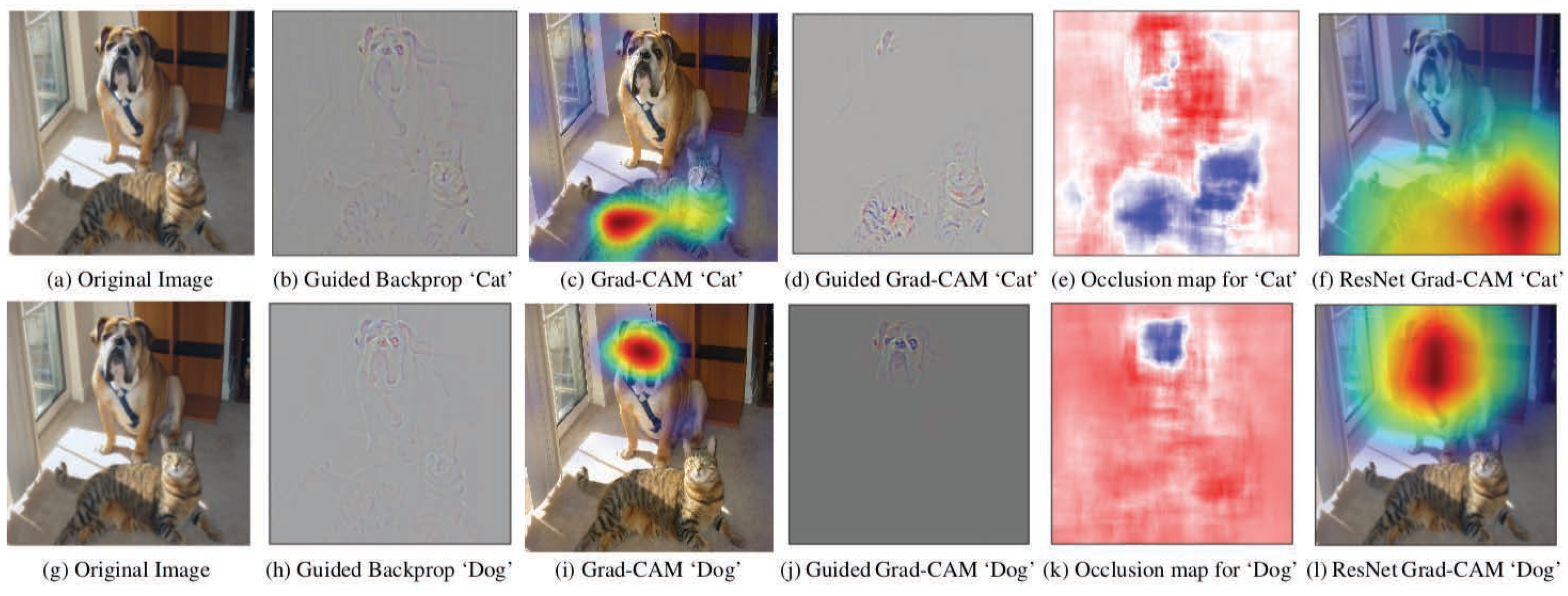
• Visualizations: To visualize an explanation, there are many options [60]. There are explainers that create visualizations that give an explanation by “digesting” the mechanisms of a model down to images, which themselves have to be interpreted. A further tool is to look at the activations produced on each layer of a trained CNN as it processes an image or video. Another one enables visualizing features at each layer of a DNN via regularized optimization in the image space [61]. Visualizations of particular neurons or neuron layers show responsible features that lead to a maximum activation or the highest possible probability of a prediction [62] and can be split into generative models or saliency maps. Salience maps of important features are calculated, and they show superpixels that have influenced the prediction most, for example [7] (Figure 6). To create a map of important pixels, one can repeatedly feed an architecture with several portions of inputs and compare the respective output, or one can visualize them directly by going rearwards through the inverted network from an output of interest;
• Grouped in this category as well is exploiting neural networks with activation atlases through feature inversion. This method can reveal how the network typically represents some concepts [63];
• Considering image or text portions that maximize the activation of interesting neurons or whole layers can lead to the interpretation of the responsible area of individual parts of the architecture.

Reference [64] defined key terms such as “explanation”, “interpretability”, and “explainability” philosophically. We want to emphasize that interpretability and explainability are not the same, although they are often used interchangeably. Explainability arises from a set of connected inference rules and includes interpretability, but not vice versa. An explanation is one of several purposes for empirical research. It is a way to uncover new knowledge and to report relationships among different aspects of the studied phenomena. Explanation attempts to answer the “why” and “how” questions and has variable explanatory power [65]. The quality of an explanation is determined by the person receiving it. It is much more concrete; facts can be described with words or formulas, while an interpretation is just a substantial formation that arises in the head. We also describe the difficulties of both interpretability and completeness, so a compromise is needed. For more details, see the following. We compiled the most important definitions of the properties of explainers and their obvious connections in a more technical way:

• An explainer or explanator [48] is a synonym for an explaining system or explaining process that gives answers to questions in understandable terms, which could, computationally, be considered a program execution trace. For instance, if the question is how a machine is working, the explainer makes the internal structure of a machine more transparent to humans. A further question could be why a prediction was made instead of another, so the explainer should point to where the decision boundaries between classes are and why particular labels are predicted for different data points [66];
• Interpretability is a substantial first step to reach the comprehension of a complex conceptat some level of detail, but is insufficient alone [64];
• Explainability includes interpretability, but this does not always apply the other way round. It provides relevant responses to questions and subdivides their meaning into terms understandable by a human [64,67]. Explainability does not refer to a human model, but it technically highlights decision-relevant parts of machine representations [68];
• Comprehensibility or understandable explanation: An understandable explanation must be created by a machine in a given time (e.g., one hour or one day) and can be comprehended by a user, who need not to be an expert, but has an educational background. The user keeps asking a finite number of questions of the machine until he/she can no longer ask why or how because he/she has a satisfactory answer; we say he/she has comprehended.
• Completeness: A complete explanation records all possible attributes from the input to the output of a model. A DNN with its millions of parameters is too complex; hence, a complete explanation would not be understandable. This makes it necessary to focus on the most important reasons and not all of them;
• Compactness: A compact explanation has a finite number of aspects. Because the parameters and operations of a DNN are finite, one can obtain a complete explanation of a DNN after a finite number of steps. That is why compactness follows from completeness if the considered connections are finite. A DNN can be explained, for instance, completely and compactly or compactly and understandably;
• Causality: This is the relationship between cause and effect; it is not a synonym for causability;
• Causability: Causability is about measuring and ensuring the quality of an explanation and refers to a human model [68].

Other, in our eyes, less gentle aspects of data-mining and machine-learning models that are mentioned in the literature are fidelity, trust, monotonicity, usability, reliability, causality, scalability, and generality. We summarize a short overview of the definitions of [48,69]: The fidelity measures how exact an interpretable model is in imitating the behavior of a black box. It is measured in terms of the accuracy score, but with respect to the outcome of the black box, similarly to the model accuracy. Another property is trust; its degree for a model increases if the model is built by respecting the constraints of monotonicity given by the user [70]. The usability influences the trust level of a model because the user tends to trust models that provide information that assists them in accomplishing a task with awareness. That is why a queryable and interactive explanation results in being more usable than a fixed, textual explanation. Reliability means that a model should have the ordinary required features to maintain certain levels of performance independently of small variations of the input data or the parameters. Causality is the ability to control changes in the input due to a perturbation affecting the model behavior. Further, Big Data require scalability, as it is opportune to have models able to scale to large input data with large input spaces. Moreover, generality means one might use the same model with different data in different application scenarios, and it is preferable to have portable models that do not require special training regimes or restrictions.

We give some examples of explaining approaches that can be placed in the last point: A global ante hoc method for tabulator data is the Bayesian Rule List (BRL) [71,72]. The BRL is a generative model that yields a posterior distribution over possible decision lists, which consist of a series of if-then statements that discretize a high-dimensional, multivariate feature space into a series of simple, readily interpretable decision statements. The “if” statements define a partition of a set of features, and the “then” statements correspond to the predicted outcome of interest. According to the authors, their experiments showed that the BRL has predictive accuracy on par with the current top algorithms for prediction in Machine Learning. The BRL is able to be used to produce highly accurate and interpretable medical scoring systems. The work was developed from preliminary versions that used a different prior, called the Bayesian list machine [73], a generative model for fitting decision lists, a type of interpretable classifier, to the data. Similar to DeepRED [74], the rule generation “KnowledgeTron” (KT) [75] applied an if-then-rule for each neuron, layer by layer, to obtain a formalized relationship between a DNN and a rule-based system. The extraction of rules is important because this allows interpreting the network’s knowledge and can regularize it and prevent it from overfitting the data.

Another option in this field is to decompose a DNN into Decision Trees, e.g., TREPAN [76] or DeepRED. TREPAN is an algorithm for extracting comprehensible, symbolic representations from trained neural networks. It queries a given network to induce a Decision Tree that describes the concept represented by the network. The authors demonstrated that TREPAN is able to produce Decision Trees that are accurate and comprehensible and maintain a high level of fidelity to the networks from which they were extracted. According to the authors of DeepRED, their method is the first attempt to extract rules and make a DNN’s decision more transparent. Decision Trees have been used since the 1990s to explain machine-learning tasks, but applied to DNNs, their generation is quite expensive and the comprehensibility suffers from the necessary increasing size and number of trees. Decision Trees are able to explain a model completely, but with DNNs, there is a conflict with comprehensibility. The problem is that incomprehensible Decision Trees are presumptively no more explanatory than the original DNN. Furthermore, the inability to encode loops makes it difficult to explain most algorithms, let alone heuristics encoded by recurrent DNNs.

2.3. Selected DNN Explainers Presented

Let us give a technical overview about the selected explanator models; we focus on the category of Computer Vision:

The Counterfactual Impact Evaluation (CIE) method [77,78] is a local method of comparison for different predictions. Counterfactuals are contrastive. They explain why a decision was made instead of another. A counterfactual explanation of a prediction may be defined as the smallest change to the feature values that changes the prediction to a predefined output. They could be employed for DNNs with any data type.

A famous work that is often associated with visualizing and understanding Convolutional Neural Networks is DeconvNet [51]: DeconvNet is a calculation of a backward convolutional network that reuses the weights at each layer from the output layer back to the input image. The employed mechanisms are deconvolution and unpooling, which are especially designed for CNNs with convolutions, max-pooling, and Rectified Linear Units (ReLUs). The method makes it possible to create feature maps of an input image that activates certain hidden units most, linked to a particular prediction; see Figure 5. With their propagation technique, they identified the most responsible patterns for this output. The patterns are visualized in the input space. DeconvNet is limited to max-pooling layers, but the unpooling uses an approximate inverse. A particular theoretical criterion that could directly connect the prediction to the created input patterns is missing. To close that gap, Reference [55] proposed a new and efficient way following the initial attempt of Zeiler and Fergus. They replaced max-pooling by a convolutional layer with an increased stride and called the method the All Convolutional Net. The performance on image recognition benchmarks was similar as well. With this approach, they were able to analyze the neural network by introducing a novel variant of DeconvNet to visualize the concepts learned by higher network layers of the CNN. The problem of max-pooling layers is that they are not invertible in general. That is the reason why Zeiler and Fergus computed positions of maxima within each pooling region and used these “switches” in DeconvNet for a discriminative reconstruction. Not using max-pooling, Springenberg et al. could directly display learned features without being conditioned on an image. Furthermore, for higher layers, they produced sharper, more recognizable visualizations of descriptive image regions than previous methods. This is in agreement with the fact that higher layers learn more invariant representations. Nie et al. [79] criticized DeconvNet or methods such as GBP for generating more human-interpretable visualizations instead of class-sensitive ones than the map. They carried out only a partial image reconstruction, not emphasizing class-relevant pixels or presenting the learned weights, thus providing no added or explanatory value. In their work, the authors began with a random three-layer CNN and later generalized it to more realistic cases. They explained that both GBP and DeconvNet are basically performing partial image recovery, which verifies their class-insensitive properties, unlike the saliency map. In addition to this, DeconvNet relies on max-pooling to recover the input. Nie et al. revealed that it is the backward ReLU, used by both GBP and DeconvNet, along with the local connections in CNNs that are responsible for the human-interpretable visualizations. Finally, the authors concluded in principle that DeconvNet or GBP is unrelated to the decision-making of neural networks.

Yosinski et al. [61] introduced two tools to aid the interpretation of DNNs in a global way. First, they displayed the neurons’ activations produced at each layer of a trained CNN processing an image or sequence of images. They found that looking at live activations that change in response to the input images helps build valuable intuitions about the inner mechanisms of these neural networks. The second tool was built on previous versions that calculated less recognizable images. Some novel regularization methods that were combined produced qualitatively clearer and more interpretable visualizations and enabled plotting features at each layer via regularized optimization in the image space.

A gradient-based method is Layerwise Relevance Propagation (LRP) [53], which suffers from the shattered gradients problem; see Figure 7. It relies on a conservation principle to propagate the outcome decision back without using gradients. The idea behind it is a decomposition of prediction function as a sum of layerwise relevance values. When LRP is applied to deep ReLU networks, LRP can be understood as a deep Taylor decomposition of the prediction. This principle ensures that the prediction activity is fully redistributed through all the layers onto the input variables. For more about how to explain nonlinear classification decisions with deep Taylor decomposition, see [54]. They decomposed the network classification decision into the contributions of its input elements and assessed the importance of single pixels in image classification tasks. Their method efficiently utilizes the structure of the network by backpropagating the explanations from the output to the input layer and displaying the connections in heat maps. Reference [60] investigated different methods to compute heat maps in Computer Vision applications. They concluded that layerwise relevance propagation (e.g., LRP) is qualitatively and quantitatively superior in explaining what made a DNN arrive at a particular classification decision to the sensitivity-based approaches or the deconvolution methods [51]. The inferior methods were much noisier and less suitable for identifying the most important regions with respect to the classification task. Their work did not give an answer about how to make a more detailed analysis of the prioritization of image regions or even how to quantify the heat map quality. Reference [80] criticized that the explaining methods DeconvNet, guided backpropagation, and LRP do not produce the theoretically correct explanation for a linear model and their contributions to understanding were scarce. Based on an analysis of linear models (see also [54,81]), they proposed a generalization that yielded the two neuronwise explanation techniques PatternNet (for signal visualization) and PatternAttribution (for decomposition methods) by taking the data distribution into account. They demonstrated that their methods were sound and constitute a theoretical, qualitative, and quantitative improvement towards explaining and understanding DNNs.

Furthermore, a global and ante hoc model is a joint framework for description and prediction, presented by [82]. The model creates Black box Explanations through Transparent Approximations (BETAs). It learns a compact two-level decision set in which each rule explains parts of the model behavior unambiguously and is a combined objective function to optimize these aspects: high agreement between the explanation and the model; little overlap between the decision rules in the explanation; the explanation decision set is lightweight and small.

An interpretable end-to-end explainer for healthcare is the REverse Time AttentIoN mechanism RETAIN [83] for application to Electronic Health Record (EHR) data. The approach mimics physician practice by attending to the EHR data. Two RNNs are trained in a reverse time order with the goal of efficiently generating the appropriate attention variables. It is based on a two-level neural attention generation process that detects influential past visits and significant clinical variables to improve accuracy and interpretability.

Another technique was realized by [59]. To find prototype class members, they created input images that had the highest probability of being predicted as certain classes of a trained CNN (Figure 8). Their tools were Taylor series, based on partial derivatives to display input sensitivities in images. A few years later, Reference [58] developed this idea further by synthesizing the preferred inputs for neurons in neural networks via deep generator networks for activation maximizing. The first algorithm is the generator and creates synthetic prototype class members that look real. The second algorithm is the black box classifier of the artificial image whose classification probability should be maximized. To view the prototype images, see Figure 9. Another related derivative-based method is DeepLift [84]. It propagates activation differences instead of gradients through the network. Partial derivatives do not explain a single decision, but point to what change in the image could make a change in the prediction.

Reference [85] showed that some convolutional layers behave as unsupervised object detectors. They used global average pooling and created heat maps of a pre-softmax layer that pointed out the regions of an image that were responsible for a prediction. The method is called Class Activation Mapping (CAM). On this was created Gradient-weighted Class Activation Mapping (Grad-CAM) [86] (see Figure 10), which is applicable to several CNN model families, classification, image captioning, visual question answering, reinforcement learning, or re-training. An outcome decision can be explained by Grad-CAM by using the gradient information to understand the importance of each neuron in the last convolutional layer of the CNN. The Grad-CAM localizations are combined with existing high-resolution visualizations to obtain guided Grad-CAM visualizations that are both high-resolution, as well as class discriminative. On the methods CAM and Grad-CAM was built Grad-CAM++ [87], which gives human-interpretable visual explanations of CNN-based predictions of multiple tasks such as classification, image captioning, or action recognition. Grad-CAM++ composites the positive partial derivatives of feature maps of a convolutional rear layer with a weighted special class score. The method can provide better visual explanations of CNN predictions, in particular better object localization, and explains by considering the occurrence of multiple object instances in an image.

To mark the most responsible pixels or areas of pixels of an image for a special class prediction, it is a promising idea to increase human understanding. The approach of [88] focuses on single words of a caption generated by an RNN and highlighted the region of the image that is most important for this word; see Figure 11. It displays a visualization of an attention map by a highlighted region for the word “dog” of the associated image caption “A dog is standing on a hardwood floor”. The underlying mechanism relies on a combination of RNN and cross-attention, trained for the task of generating a caption for the given image. Corresponding data are required for such a task, i.e., the combination of images and their associated captions. The explanation is right, although the caption of the classifier is not totally correct because the dog is lying on the floor and not standing. An explainer just explains a given prediction or a certain part of it, independent if it being wrong or not. A person can use it to check various criticisms, but it is not built to automatically verify or rate its use for bias detection and the identification of adversarial attacks or even debug it.

Much more general is Local Interpretable Model-agnostic Explanations (LIMEs), presented by [7], which can explain the predictions of any agnostic black box classifier and any data; see Figure 6. This is a post hoc, local model, being interpretable and model-agnostic. LIMEs focus on feature importance and give outcome explanations: they highlight the superpixels of the regions of the input image or the words from a text or table that are relevant for the given prediction. While the model complexity is kept low, the model minimizes the distance of the explanation to the prediction. This ensures a trade-off between interpretability and local fidelity. A challenge for transparency is that LIMEs are themselves a black box, and Reference [89] pointed to the poor performance of LIMEs regarding their proposed evaluation metrics correctness, consistency, and confidence in comparison to the other considered explainers Grad-CAM, Smooth-Grad, and IG (described in the following). Furthermore, one can explain only images that can be split into superpixels. The authors did not describe how to explain video object detection or segmentation networks. An interesting approach is a prototype evaluator on LIMEs. The Submodular Pick (SP-LIME) model judges whether you can trust the whole model or not. It selects a picked diverse set of representative instances with LIMEs via submodular optimization. The user should evaluate the black box by regarding the feature words of the selected instances. It is conceivable that it also recognizes bias or systematic susceptibility to adversarial examples. With this knowledge, it is also possible to improve a bad model. SP-LIME was researched with text data, but the authors claimed that it can be transferred to models for any data type.

Another approach that focuses on the most discriminative region in an image to explain an automatic decision is Deep Visual Explanation (DVE) [90]; see Figure 12. This was inspired by CAM and Grad-CAM and tested the explanator on randomly chosen images from the COCO dataset [91], applied to the pre-trained neural network VGG-16 using the Kullback–Leibler (KL) divergence [92]. They captured the discriminative areas of the input image by considering the activation of high and low spatial scales in the Fourier space.

With their conditional multivariate model Prediction Difference Analysis (PDA), Reference [93] concentrated on explaining visualizations of natural and medical images in classification tasks. Their goal was to improve and interpret DNNs. Their technique was based on the univariate approach of [94] and the idea that the relevance of an input feature with respect to a class can be estimated by measuring how the prediction changes if the feature is removed. Zintgraf et al. removed several features at one time using their knowledge about the images by strategically choosing patches of connected pixels as the feature sets. Instead of going through all individual pixels, they considered all patches of a special size implemented in a sliding window fashion. They visualized the effects of different window sizes and marginal versus conditional sampling and displayed feature maps of different hidden layers and top-scoring classes.

Reference [95] described Smooth-Grad, which reduces visual noise and, hence, improves visual explanations about how a DNN is making a classification decision. Comparing their work to several gradient-based sensitivity map methods such as LRP, DeepLift, and Integrated Gradients (IG) [96], which estimate the global importance of each pixel and create saliency maps, showed that Smooth-Grad focuses on local sensitivity and calculates averaging maps with a smoothing effect made from several small perturbations of an input image. The effect is enhanced by further training with these noisy images and finally having an impact on the quality of sensitivity maps by sharpening them. The work of [89] evaluated the explainers LIME, Grad-CAM, Smooth-Grad, and IG with regard to the properties correctness, consistency, and confidence and came to the result that Grad-CAM often performs better than others.

To improve and expand the understanding of Multimodal Explanation (ME) [97], a local, post hoc approach gave visual and textual justifications of the predictions with the help of two novel explanation datasets through crowd sourcing. The employed tasks were classification decisions for activity recognition and visual question answering; see Figure 13. The visual explanation was created by an attention mechanism that conveyed knowledge about what region of the image was important for the decision. This explanation guides the generation of the textual justification out of a LSTM feature, which is a prediction of a classification problem over all possible justifications.

A new and extensive visualized approach was created by [98] (see Figure 14), showing what features a Deep-Learning model has learned and how those features interact to make predictions. Their model is called Summit and combines two scalable tools: (1) activation aggregation discovers important neurons; (2) neuron-influenced aggregation identifies relationships among such neurons. An attribution graph that reveals and summarizes crucial neuron associations and substructures that contribute to a model’s outcomes is created. Summit combines famous methods such as computing synthetic prototypes of features and showing examples from the dataset that maximize special neurons of different layers. Deeper in the graph, it is examined how the low-level features combine to create high-level features. Novel as well is that it exploits neural networks with activation atlases [63]; see Figure 15. This method uses feature inversion to visualize millions of activations from an image classification network to create an explorable activation atlas of features the network has learned. Their approach is able to reveal visual abstractions within a model and even high-level misunderstandings in a model that can be exploited. Activation atlases are a novel way to peer into convolutional vision networks and represents a global, hierarchical, and human-interpretable overview of concepts within the hidden layers.

Just in the last few months, the importance of interpretability has been growing, which is why there appeared several single studies, investigating the contribution of some aspects of a neural network such as the impact of color [99], texture [24], etc., without explaining a whole model extensively, however, which all contribute to a deeper understanding.

In

Table 1. Overview of some explainers for DNNs. Ordered by model resp. paper name, reference (author and year), data type, main method, and main properties.

Model	Authors	Data	Method	Properties
Deep Inside	[59]	image	saliency mask	local, post hoc
DeconvNet	[51]	image	gradients	global, post hoc
All-CNN	[55]	image	gradients	global, post hoc
Deep Visualization	[61]	image	neurons activation	global, ante hoc
Deep Learning	[88]	image	visualization	local, post hoc
Show, attend, tell	[100]	image	saliency mask	local, ante hoc
LRP	[53]	image	decomposition	local, ante hoc
CAM	[85]	image	saliency mask	local, post hoc
Deep Generator	[58]	image	gradients, prototype	local, ante hoc
Interpretable DNNs	[101]	image	saliency map	local, ante hoc
VBP	[102]	image	saliency maps	local, post hoc
DTD	[54]	image	decomposition	local, post hoc
Meaningful	[103]	image	saliency mask	local, post hoc, agn.
PDA	[93]	image	feature importance	local, ante hoc
DVE	[92]	image	visualization	local, post hoc
Grad-CAM	[86]	image	saliency mask	local, post hoc
Grad-CAM++	[87]	image	saliency mask	local, post hoc
Smooth-Grad	[95]	image	sensitivity analysis	local, ante hoc
ME	[97]	image	visualization	local, post hoc
Summit	[98]	image	visualization	local, ante hoc
Activation atlases	[63]	image	visualization	local, ante hoc
SP-LIME	[7]	text	feature importance	local, post hoc
Rationalizing	[104]	text	saliency mask	local, ante hoc
Generate reviews	[105]	text	neurons activation	global, ante hoc
BRL	[71]	tabular	Decision Tree	global, ante hoc
TreeView	[106]	tabular	Decision Tree	global, ante hoc
IP	[107]	tabular	neurons’ activation	global, ante hoc
KT	[75]	any	rule extraction	global, ante hoc
Decision Tree	[27]	any	Decision Tree	global, ante hoc, agn.
CIE	[77]	any	feature importance	local, post hoc
DeepRED	[74]	any	rule extraction	global, ante hoc
LIME	[7]	any	feature importance	local, post hoc, agn.
NES	[108]	any	rule extraction	local, ante hoc
BETA	[82]	any	Decision Tree	global, ante hoc
PALM	[109]	any	Decision Tree	global, ante hoc
DeepLift	[84]	any	feature importance	local, ante hoc
IG	[96]	any	sensitivity analysis	global, ante hoc
RETAIN	[83]	EHR	reverse time atten.	global, ante hoc

, we give an overview of the presented explainers of DNNs, sorted by date and year. The main techniques and properties are mentioned for a brief comparison. The property model-agnostic is abbreviated as agn. You can initially orientate yourself first on the type of data and desired method to find a suitable model. It makes sense to choose a further developed variant in each case, e.g., the All Convolutional Net instead of DeconvNet or GRAD-Cam instead of LIME, IG, or Smooth-Grad.

2.4. Analysis of Understanding and Explaining Methods

We still wanted to go into studies on the general analysis of explainability and machine understanding and considered some survey papers.

With an overview of the interpretability of Machine Learning, Reference [64] try to explain explanations. They defined some key terms and reviewed a number of approaches towards classical explainable AI systems, also focusing on Deep Learning tasks. Furthermore, they investigated the role of single layers, individual units, and representation vectors in the explanation of deep network representations. Finally, they presented a taxonomy that examined what is being explained by these explanations. They summarized that it is not obvious what the best purpose or type of explanation metric is and should be and gave advice to combine explaining ideas from different fields.

Another approach towards understanding is to evaluate the human interpretability of explanation [110]. They investigated the consistence of the output of an ML system with its input and the supposed rationale. Therefore, they carried out user studies to identify what kinds of increases in complexity have the most dominant effect on the time humans need to take to verify the rationale and which seem to be more insensitive. Their study quantified what kind of explanation makes them be the most understandable by humans. As a main result, they found that in general, greater complexity results in higher response times and lower satisfaction.

Even simple interpretable explainers do not mostly quantify if the user can trust them. A study on trust in black box models and post hoc explanations [111] provided the main problems in the literature and the kind of black box systems. They evaluated three different explanation approaches: (1) based on the users’ initial trust, (2) the users’ trust in the provided explanation of three different post hoc explanator approaches, and (3) the established trust in the black box by a within-subject design study. The participants were asked if they trust that a special model works well in the real world, if they suppose it to be able to distinguish between the classes, and why. The results of their work led to the conclusion that although the black box prediction model and explanation are independent of each other, trusting the explanation approach is an important aspect of trusting the prediction model.

A discussion of some existing approaches to perturbation analysis was given in the study of [112]; see Figure 16. Their work, based on [103], found an adversarial effect of perturbations on the network’s output. Extremal perturbations are regions of an input image that maximally affect the activation of a certain neuron in a DNN. Measuring the effects of perturbations of the image is an important family of attribution methods. Attribution aims at characterizing the response of a DNN by looking at which parts of the network’s input are the most responsible ones for determining its prediction, which is mostly performed by several kinds of backpropagation. Fong et al. investigated their effect as a function of the area. In particular, they visualized the difference between perturbed and unperturbed activations using a representation inversion technique. They introduced TorchRay [113], a PyTorch interpretability library.

Fan et al. [114] reviewed the key ideas, implications, and limitations of existing interpretability studies. They proposed a comprehensive taxonomy for interpretation methods with a focus on medicine. To overcome the vulnerabilities of existing deep reconstruction networks, while at the same time transferring the interpretability of the model-based methods to the hybrid DNNs, they used their recently proposed ACID framework. This allows a synergistic integration of data-driven priors and Compressed Sensing (CS)-modeled priors. Some results are visualized from their own implementation and link to open-sourced relevant codes on GitHub; see [115]. Finally, they concluded that a unified and accountable interpretation framework is critical to elevate interpretability research to a new level.

In their work, Burkart and Huber [116] offered a formalization of different explanation approaches and a review of the corresponding classification and regression literature for the entire explanation chain. They gave reasons for explainability and the assessment of it and introduced example domains demanding XAI. Concepts and definitions were worked out. In the main part, surrogate models, where the explanation is directly inferred from the black box model, were described. In addition to this, the authors specified approaches that can directly generate an explanation. Various aspects of the data, data quality, and ontologies were highlighted as well. The conclusion of this extensive study was that the most one can strive for when giving an explanation is a sort of human-graspable approximation of the decision process. This is the reason why in an explanation, all sorts of environmental conditions play a role, as the person telling the story seeks to build trust in and understanding of her/his decision.

Another paper [117] presented an overview of interpretable approaches and defined new characteristics of interpretable ML, for example privacy, robustness, causality, or faith. Related open-source software tools help to explore and understand the behavior of the ML models and to describe enigmatic and unclear ML models. These tools assist in constructing interpretable models and include a variety of interpretable ML methods that assist people with understanding the connection between input and output variables through interpretation and validating the decision of a predictive model to enable lucidity, accountability, and fairness in the algorithmic decision-making policies.

2.5. Open Problems in Understanding DNNs and Future Work

When summarizing the functionality of explainers, one notices that some facts are hard to measure: First, the time, which is needed to understand the decision, is difficult to obtain. Local working explainers can deliver a root case for each prediction, but: How many examples are necessary to look at, to be sure, that all results and thereby the black box is faithful? In addition to this, the model complexity of several explainers is different. The complexity is often calculated as a term opposed to interpretability. The complexity of a black box can be expressed, for instance, as the number of non-zero weights in neural networks or the depth of trees for the decision. However, the complexity of the explanation could depend on the complexity of the black box.

More work must be performed also in data exploration: Interpretable data in the mentioned papers are mainly images, texts, and tabular data, which are all easily interpretable data for humans. Missing is general data such as vectors, matrices, or complex spatiotemporal numbers. Of course, they have to be transformed before analyzing to be understandable for our brains. Sequences, networks, etc., could be the inputs to a black box, but until now, such models have not been explained.

There is no agreement on how to quantify the quality and grade of explanation. These are open problems. It is a challenge to develop appropriate suitable vocabularies of the explainer and align them with the semantics and vocabulary of the domain. Some metrics to evaluate explainers have been proposed, e.g., causability ([68] or [89]), but unfortunately, many of them tend to suffer from major drawbacks such as the computational cost [118] or simply focusing on one desirable attribute of a good explainer [119]. However, a definition with the properties of a DNN model such as reliability, soundness, completeness, compactness, comprehensibility, and the knowledge of the breaking points of an algorithm is still missing. This is uniquely difficult for DNNs because of their deep nonlinear structure and the huge number of parameters that have to be optimized and ultimately explained in a consistent, understandable, and transparent manner. However, to describe the necessary properties of a model, there is a need to focus on uniform definitions. It is important to consider the robustness, which indicates how robust the system is to small changes of the architecture or the test data [67,120], and this could be a reference to reliability. To compare or even evaluate models, also fairness, which requires that the model guarantees the protection of groups against discrimination [48], and reliability need to be quantified. In addition to this, an evaluator that detects bias or identifies and fends off adversarial attacks would be beneficial. Our further work will be performed here.

3. Conclusions

In this paper, we summarized state-of-the-art explainers and survey manuscripts on Deep Neural Networks. First, we gave reasons why it is necessary to comprehend black box DNNs: adversarial attacks that are not understandable by humans pose a serious threat to the robustness of DNNs. Furthermore, we expounded on why models learn prejudices caused by contaminated training data; hence, through widespread application, they could be partly responsible for increased unfairness. On the other hand, novel laws demand for the right of users to ask how intelligent decision-making systems arrive at their decisions. One first solution was the development of explainers. We gave a taxonomic introduction to the main definitions, properties, tools, and methods of explaining systems. Unlike others—to our best knowledge—we focused on proven explaining models, mostly in the area of Computer Vision, and explained their development and pros and cons. We presented different representations of explanations and differentiated the explainers with regard to the application, data, and properties. Finally, we introduced surveys and studies that analyzed or evaluated explaining systems and tried to quantify machine understanding in general. This leads to the realization that uniform definitions and evaluating systems for explainers are still needed to solve open problems. Finally, the outlook for further ideas such as quantifying the grade of explanation or directly evaluating models makes this work valuable.

References

1. Das, A.; Rad, P. Opportunities and challenges in explainable artificial intelligence (xai): A survey. arXiv 2020, arXiv:2006.11371. [Google Scholar]
2. Chen, Y.; Ouyang, L.; Bao, F.S.; Li, Q.; Han, L.; Zhu, B.; Ge, Y.; Robinson, P.; Xu, M.; Liu, J.; et al. An interpretable machine learning framework for accurate severe vs. non-severe COVID-19 clinical type classification. Lancet 2020. [Google Scholar] [CrossRef]
3. Fan, X.; Liu, S.; Chen, J.; Henderson, T.C. An investigation of COVID-19 spreading factors with explainable ai techniques. arXiv 2020, arXiv:2005.06612. [Google Scholar]
4. Karim, M.; Döhmen, T.; Rebholz-Schuhmann, D.; Decker, S.; Cochez, M.; Beyan, O. Deepcovidexplainer: Explainable COVID-19 predictions based on chest X-ray images. arXiv 2020, arXiv:2004.04582. [Google Scholar]
5. Szegedy, C.; Zaremba, W.; Sutskever, I.; Bruna, J.; Erhan, D.; Goodfellow, I.; Fergus, R. Intriguing properties of neural networks. arXiv 2013, arXiv:1312.6199. [Google Scholar]
6. Goodfellow, I.J.; Shlens, J.; Szegedy, C. Explaining and harnessing adversarial examples. arXiv 2014, arXiv:1412.6572. [Google Scholar]
7. Ribeiro, M.T.; Singh, S.; Guestrin, C. Why should i trust you? Explaining the predictions of any classifier. In Proceedings of the 22nd ACM SIGKDD International Conference on Knowledge Discovery and Data Mining, San Francisco, CA, USA, 13–17 August 2016. [Google Scholar]
8. Moosavi-Dezfooli, S.M. DeepFool: A simple and accurate method to fool deep neural networks. In Proceedings of the IEEE Conference on Computer Vision and Pattern Recognition, Las Vegas, NV, USA, 27–30 June 2016. [Google Scholar]
9. Bose, A.J.; Aarabi, P. Adversarial attacks on face detectors using neural net based constrained optimization. In Proceedings of the IEEE 20th International Workshop on Multimedia Signal Processing (MMSP), Vancouver, BC, Canada, 29–31 August 2018. [Google Scholar]
10. Jia, R.; Liang, P. Adversarial examples for evaluating reading comprehension systems. arXiv 2017, arXiv:1707.07328. [Google Scholar]
11. Eykholt, K.; Evtimov, I.; Fernandes, E.; Li, B.; Rahmati, A.; Xiao, C.; Prakash, A.; Kohno, T.; Song, D. Robust physical-world attacks on deep learning visual classification. In Proceedings of the IEEE Conference on Computer Vision and Pattern Recognition, Salt Lake City, UT, USA, 18–23 June 2018. [Google Scholar]
12. Ranjan, A.; Janai, J.; Geiger, A.; Black, M.J. Attacking Optical Flow. In Proceedings of the International Conference on Computer Vision, Seoul, Korea, 27–28 October 2019. [Google Scholar]
13. Sharif, M.; Bhagavatula, S.; Bauer, L.; Reiter, M.K. Accessorize to a crime: Real and stealthy attacks on state-of-the-art face recognition. In Proceedings of the ACM SIGSAC Conference on Computer and Communications Security, Vienna, Austria, 24–28 October 2016. [Google Scholar]
14. Sharif, M.; Bhagavatula, S.; Bauer, L.; Reiter, M.K. A General Framework for Adversarial Examples with Objectives. ACM Trans. Priv. Secur. (TOPS) 2019, 22, 1–30. [Google Scholar] [CrossRef]
15. Goodman, F. European union regulations on algorithmic decision-making and a right to explanation. In Proceedings of the ICML Workshop on Human Interpretability in ML, New York, NY, USA, 23 June 2016. [Google Scholar]
16. Muller, H.; Mayrhofer, M.T.; Van Veen, E.B.; Holzinger, A. The Ten Commandments of ethical medical AI. Computer 2021, 54, 119–123. [Google Scholar] [CrossRef]
17. Holmes, J.; Meyerhoff, M. The Handbook of Language and Gender; John Wiley & Sons: Hoboken, NJ, USA, 2008. [Google Scholar]
18. Bolukbasi, T.; Chang, K.W.; Zou, J.Y.; Saligrama, V.; Kalai, A.T. Man is to computer programmer as woman is to homemaker? debiasing word embeddings. Adv. Neural Inf. Process. Syst. 2016, 29, 4349–4357. [Google Scholar]
19. Hirschberg, J.; Manning, C.D. Advances in natural language processing. Science 2015, 349, 261–266. [Google Scholar] [CrossRef]
20. Greenwald, A.G.; McGhee, D.E.; Schwartz, J.L. Measuring individual differences in implicit cognition: The implicit association test. J. Personal. Soc. Psychol. 1998, 74, 1464–1480. [Google Scholar] [CrossRef]
21. Chakraborty, T.; Badie, G.; Rudder, B. Reducing Gender Bias in Word Embeddings. Computer Science Department, Stanford University. 2016. Available online: http://cs229.stanford.edu/proj2016/report/ (accessed on 15 March 2018).
22. Font, J.E.; Costa-Jussa, M.R. Equalizing gender biases in neural machine translation with word embeddings techniques. arXiv 2019, arXiv:1901.03116. [Google Scholar]
23. Nguyen, A.; Yosinski, J.; Clune, J. Deep Neural Networks are Easily Fooled: High Confidence Predictions for Unrecognizable Images. In Proceedings of the IEEE Conference on Computer Vision and Pattern Recognition, Boston, MA, USA, 7–12 June 2015. [Google Scholar]
24. Geirhos, R.; Rubisch, P.; Michaelis, C.; Bethge, M.; Wichmann, F.A.; Brendel, W. ImageNet-trained CNNs are biased towards texture; Increasing shape bias improves accuracy and robustness. arXiv 2018, arXiv:1811.12231. [Google Scholar]
25. Hastie, T.; Tibshirani, R. Generalized additive model (GAM). Stat. Sci. 1986, 1, 297–318. [Google Scholar]
26. Breiman, L.; Friedman, J.; Olshen, R.; Stone, C. Classification and Regression Trees. Monterey; Wadsworth International Group: Monterey, CA, USA, 1984. [Google Scholar]
27. Friedman, J.; Hastie, T.; Tibshirani, R. The Elements of Statistical Learning; Springer Series in Statistics New York; Springer: New York, NY, USA, 2001. [Google Scholar]
28. Salzberg, S.L. C4. 5: Programs for Machine Learning by J. Ross Quinlan. Morgan Kaufmann Publishers, Inc., 1993; Kluwer Academic: Boston, MA, USA, 1994. [Google Scholar]
29. Friedman, J.H. Greedy function approximation: A gradient boosting machine. Ann. Stat. 2001, 29, 1189–1232. [Google Scholar] [CrossRef]
30. Goldstein, A.; Kapelner, A.; Bleich, J.; Pitkin, E. Peeking inside the black box: Visualizing statistical learning with plots of individual conditional expectation. J. Comput. Graph. Stat. 2015, 24, 44–65. [Google Scholar] [CrossRef]
31. Van Lent, M.; Fisher, W.; Mancuso, M. An explainable artificial intelligence system for small-unit tactical behavior. In Proceedings of the National Conference on Artificial Intelligence, San Jose, CA, USA, 25–29 July 2004. [Google Scholar]
32. Shortliffe, E.H. Mycin: A knowledge-based computer program applied to infectious diseases. In Proceedings of the Annual Symposium on Computer Application in Medical Care, San Francisco, CA, USA, 5 October 1997; American Medical Informatics Association: Bethesda, MD, USA, 1977. [Google Scholar]
33. Baehrens, D.; Schroeter, T.; Harmeling, S.; Kawanabe, M.; Hansen, K.; MÞller, K.R. How to explain individual classification decisions. J. Mach. Learn. Res. 2010, 11, 1803–1831. [Google Scholar]
34. Breiman, L. Random forests. Mach. Learn. 2001, 45, 5–32. [Google Scholar] [CrossRef] [Green Version]
35. Kononenko, I. Inductive and Bayesian learning in medical diagnosis. Appl. Artif. Intell. Int. J. 1993, 7, 317–337. [Google Scholar] [CrossRef]
36. Becker, B.; Kohavi, R.; Sommerfield, D. Visualizing the simple Bayesian classifier. In Information Visualization in Data Mining and Knowledge Discovery; Morgan Kaufmann Publishers Inc.: San Francisco, CA, USA, 2001; pp. 237–249. Available online: https://dl.acm.org/doi/10.5555/383784.383809 (accessed on 7 October 2021).
37. Možina, M.; Demšar, J.; Kattan, M.; Zupan, B. Nomograms for visualization of naive Bayesian classifier. In European Conference on Principles of Data Mining and Knowledge Discovery, Proceedings of the 8th European Conference on Principles and Practice of Knowledge Discovery in Databases, Pisa, Italy, 20–24 September 2004; Springer: Berlin/Heidelberg, Germany, 2004. [Google Scholar]
38. Poulet, F. Svm and graphical algorithms: A cooperative approach. In Proceedings of the Fourth IEEE International Conference on Data Mining (ICDM’04), Brighton, UK, 1–4 November 2004. [Google Scholar]
39. Hamel, L. Visualization of support vector machines with unsupervised learning. In Proceedings of the IEEE Symposium on Computational Intelligence and Bioinformatics and Computational Biology, Toronto, ON, Canada, 28–29 September 2006. [Google Scholar]
40. Breiman, L. Bagging predictors. Mach. Learn. 1996, 24, 123–140. [Google Scholar] [CrossRef] [Green Version]
41. Ciresan, D.; Giusti, A.; Gambardella, L.M.; Schmidhuber, J. Deep neural networks segment neuronal membranes in electron microscopy images. Adv. Neural Inf. Process. Syst. 2012, 25, 2843–2851. [Google Scholar]
42. Ciresan, D.; Meier, U.; Schmidhuber, J. Multi-column deep neural networks for image classification. In Proceedings of the IEEE Conference on Computer Vision and Pattern Recognition, Providence, RI, USA, 16–21 June 2012. [Google Scholar]
43. Le, Q.V.; Zou, W.Y.; Yeung, S.Y.; Ng, A.Y. Learning hierarchical invariant spatio-temporal features for action recognition with independent subspace analysis. In Proceedings of the CVPR 2011, Colorado Springs, CO, USA, 20–25 June 2011. [Google Scholar]
44. Krizhevsky, A.; Sutskever, I.; Hinton, G.E. Imagenet classification with deep convolutional neural networks. Adv. Neural Inf. Process. Syst. 2012, 25, 1097–1105. [Google Scholar] [CrossRef]
45. Rumelhart, D.E.; Hinton, G.E.; Williams, R.J. Learning representations by back-propagating errors. Nature 1986, 323, 533–536. [Google Scholar] [CrossRef]
46. Collobert, R.; Weston, J.; Bottou, L.; Karlen, M.; Kavukcuoglu, K.; Kuksa, P. Natural language processing (almost) from scratch. J. Mach. Learn. Res. 2011, 12, 2493–2537. [Google Scholar]
47. Hochreiter, S.; Schmidhuber, J. Long short-term memory. Neural Comput. 1997, 9, 1735–1780. [Google Scholar] [CrossRef]
48. Guidotti, R.; Monreale, A.; Ruggieri, S.; Turini, F.; Giannotti, F.; Pedreschi, D. A survey of methods for explaining black box models. ACM Comput. Surv. (CSUR) 2019, 51, 1–42. [Google Scholar] [CrossRef] [Green Version]
49. Goebel, R.; Chander, A.; Holzinger, K.; Lecue, F.; Akata, Z.; Stumpf, S.; Kieseberg, P.; Holzinger, A. Explainable AI: The new 42? In International Cross-Domain Conference for Machine Learning and Knowledge Extraction, Proceedings of the Second IFIP TC 5, TC 8/WG 8.4, 8.9, TC 12/WG 12.9 International Cross-Domain Conference, CD-MAKE 2018, Hamburg, Germany, 27–30 August 2018; Springer: Cham, Switzerland, 2018. [Google Scholar]
50. Lipton, Z.C. The mythos of model interpretability. arXiv 2016, arXiv:1606.03490. [Google Scholar]
51. Zeiler, M.D.; Fergus, R. Visualizing and Understanding Convolutional Networks; Springer: Berlin/Heidelberg, Germany, 2014. [Google Scholar]
52. Mahendran, A.; Vedaldi, A. Understanding deep image representations by inverting them. In Proceedings of the IEEE Conference on Computer Vision and Pattern Recognition, Boston, MA, USA, 7–12 June 2015. [Google Scholar]
53. Bach, S.; Binder, A.; Montavon, G.; Klauschen, F.; Müller, K.R.; Samek, W. On pixel-wise explanations for non-linear classifier decisions by layerwise relevance propagation. PLoS ONE 2015, 10, e0130140. [Google Scholar] [CrossRef] [Green Version]
54. Montavon, G.; Lapuschkin, S.; Binder, A.; Samek, W.; Müller, K.R. Explaining nonlinear classification decisions with deep taylor decomposition. Pattern Recognit. 2017, 65, 211–222. [Google Scholar] [CrossRef]
55. Springenberg, J.; Dosovitskiy, A.; Brox, T.; Riedmiller, M. Striving for Simplicity: The All Convolutional Net. In Proceedings of the ICLR (Workshop Track), San Diego, CA, USA, 7–9 May 2015. [Google Scholar]
56. Zhang, R.; Isola, P.; Efros, A.A. Colorful image colorization. In European Conference on Computer Vision (ECCV), Proceedings of the 14th European Conference, Amsterdam, The Netherlands, 11–14 October 2016; Springer: Cham, Switzerland, 2016. [Google Scholar]
57. Zhang, J.; Bargal, S.A.; Lin, Z.; Brandt, J.; Shen, X.; Sclaroff, S. Top-down neural attention by excitation backprop. Int. J. Comput. Vis. 2018, 126, 1084–1102. [Google Scholar] [CrossRef] [Green Version]
58. Nguyen, A.; Dosovitskiy, A.; Yosinski, J.; Brox, T.; Clune, J. Synthesizing the preferred inputs for neurons in neural networks via deep generator networks. Adv. Neural Inf. Process. Syst. 2016, 29, 3387–3395. [Google Scholar]
59. Simonyan, K.; Vedaldi, A.; Zisserman, A. Deep inside convolutional networks: Visualising image classification models and saliency maps. arXiv 2013, arXiv:1312.6034. [Google Scholar]
60. Samek, W.; Binder, A.; Montavon, G.; Lapuschkin, S.; Müller, K.R. Evaluating the visualization of what a deep neural network has learned. IEEE Trans. Neural Networks Learn. Syst. 2016, 28, 2660–2673. [Google Scholar] [CrossRef] [Green Version]
61. Yosinski, J.; Clune, J.; Nguyen, A.; Fuchs, T.; Lipson, H. Understanding neural networks through deep visualization. arXiv 2015, arXiv:1506.06579. [Google Scholar]
62. Dosovitskiy, A.; Brox, T. Inverting visual representations with convolutional networks. In Proceedings of the IEEE Conference on Computer Vision and Pattern Recognition, Las Vegas, NV, USA, 27–30 June 2016. [Google Scholar]
63. Carter, S.; Armstrong, Z.; Schubert, L.; Johnson, I.; Olah, C. Activation Atlas. Distill 2019, 4, e15. [Google Scholar] [CrossRef]
64. Gilpin, L.H.; Bau, D.; Yuan, B.Z.; Bajwa, A.; Specter, M.; Kagal, L. Explaining explanations: An overview of interpretability of machine learning. In Proceedings of the IEEE 5th International Conference on Data Science and Advanced Analytics (DSAA), Turin, Italy, 1–3 October 2018. [Google Scholar]
65. Remler, D.K.; Van Ryzin, G.G. Research Methods in Practice: Strategies for Description and Causation; Sage Publications: Thousand Oaks, CA, USA, 2014. [Google Scholar]
66. Ridgeway, G.; Madigan, D.; Richardson, T.; O’Kane, J. Interpretable Boosted Naïve Bayes Classification; AAAI: Palo Alto, CA, USA, 1998. [Google Scholar]
67. Doshi-Velez, F.; Kim, B. Towards a rigorous science of interpretable machine learning. arXiv 2017, arXiv:1702.08608. [Google Scholar]
68. Holzinger, A.; Malle, B.; Saranti, A.; Pfeifer, B. Towards multi-modal causability with Graph Neural Networks enabling information fusion for explainable AI. Inf. Fusion 2021, 71, 28–37. [Google Scholar] [CrossRef]
69. Martens, D.; Vanthienen, J.; Verbeke, W.; Baesens, B. Performance of classification models from a user perspective. Decis. Support Syst. 2011, 51, 782–793. [Google Scholar] [CrossRef]
70. Freitas, A.A. Comprehensible classification models: A position paper. ACM SIGKDD Explor. Newsl. 2014, 15, 1–10. [Google Scholar] [CrossRef]
71. Letham, B.; Rudin, C.; McCormick, T.H.; Madigan, D. Interpretable classifiers using rules and bayesian analysis: Building a better stroke prediction model. Ann. Appl. Stat. 2015, 9, 1350–1371. [Google Scholar] [CrossRef]
72. Ustun, B.; Rudin, C. Methods and models for interpretable linear classification. arXiv 2014, arXiv:1405.4047. [Google Scholar]
73. Letham, B.; Rudin, C.; McCormick, T.H.; Madigan, D. An interpretable stroke prediction model using rules and Bayesian analysis. In Proceedings of the Workshops at the Twenty-Seventh AAAI Conference on Artificial Intelligence, Bellevue, WA, USA, 14–18 July 2013. [Google Scholar]
74. Zilke, J.R.; Mencía, E.L.; Janssen, F. DeepRED—Rule extraction from deep neural networks. In International Conference on Discovery Science, Proceedings of the 19th International Conference, DS 2016, Bari, Italy, 19–21 October 2016; Springer: Cham, Switzerland, 2016. [Google Scholar]
75. Fu, L. Rule generation from neural networks. IEEE Trans. Syst. Man Cybern. 1994, 24, 1114–1124. [Google Scholar]
76. Craven, M.; Shavlik, J.W. Extracting tree-structured representations of trained networks. Adv. Neural Inf. Process. Syst. 1996, 8, 24–30. [Google Scholar]
77. Bottou, L.; Peters, J.; Quiñonero-Candela, J.; Charles, D.X.; Chickering, D.M.; Portugaly, E.; Ray, D.; Simard, P.; Snelson, E. Counterfactual reasoning and learning systems: The example of computational advertising. J. Mach. Learn. Res. 2013, 14. [Google Scholar]
78. Hainmueller, J.; Hazlett, C. Kernel regularized least squares: Reducing misspecification bias with a flexible and interpretable machine learning approach. Politi. Anal. 2014, 22, 143–168. [Google Scholar] [CrossRef]
79. Nie, W.; Zhang, Y.; Patel, A. A theoretical explanation for perplexing behaviors of backpropagation-based visualizations. In Proceedings of the International Conference on Machine Learning, Stockholm, Sweden, 10–15 July 2018; pp. 3809–3818. [Google Scholar]
80. Kindermans, P.J.; Schütt, K.T.; Alber, M.; Müller, K.R.; Erhan, D.; Kim, B.; Dähne, S. Learning how to explain neural networks: Patternnet and patternattribution. arXiv 2017, arXiv:1705.05598. [Google Scholar]
81. Haufe, S.; Meinecke, F.; Görgen, K.; Dähne, S.; Haynes, J.D.; Blankertz, B.; Bießmann, F. On the interpretation of weight vectors of linear models in multivariate neuroimaging. Neuroimage 2014, 87, 96–110. [Google Scholar] [CrossRef] [Green Version]
82. Lakkaraju, H.; Bach, S.H.; Leskovec, J. Interpretable decision sets: A joint framework for description and prediction. In Proceedings of the 22nd ACM SIGKDD International Conference on Knowledge Discovery and Data Mining, San Francisco, CA, USA, 13–17 August 2016. [Google Scholar]
83. Choi, E.; Bahadori, M.T.; Sun, J.; Kulas, J.; Schuetz, A.; Stewart, W. Retain: An interpretable predictive model for healthcare using reverse time attention mechanism. In Proceedings of the 30th International Conference on Neural Information Processing Systems, Barcelona, Spain, 5–10 December 2016. [Google Scholar]
84. Shrikumar, A.; Greenside, P.; Kundaje, A. Learning important features through propagating activation differences. In Proceedings of the 34th International Conference on Machine Learning, Sydney, Australia, 6–11 August 2017; Volume 70. [Google Scholar]
85. Zhou, B.; Khosla, A.; Lapedriza, A.; Oliva, A.; Torralba, A. Learning deep features for discriminative localization. In Proceedings of the IEEE Conference on Computer Vision and Pattern Recognition, Las Vegas, NV, USA, 27–30 June 2016. [Google Scholar]
86. Selvaraju, R.R.; Cogswell, M.; Das, A.; Vedantam, R.; Parikh, D.; Batra, D. Grad-cam: Visual explanations from deep networks via gradient-based localization. In Proceedings of the IEEE International Conference on Computer Vision, Venice, Italy, 22–29 October 2017. [Google Scholar]
87. Chattopadhyay, A.; Sarkar, A.; Howlader, P.; Balasubramanian, V. Grad-CAM++: Generalized Gradient-based Visual Explanations for Deep Convolutional Networks. In Proceedings of the IEEE Winter Conference on Applications of Computer Vision (WACV), Lake Tahoe, NV, USA, 12–15 March 2018. [Google Scholar]
88. LeCun, Y.; Bengio, Y.; Hinton, G. Deep learning. Nature 2015, 521, 436–444. [Google Scholar] [CrossRef] [PubMed]
89. Anonymous. On Evaluating Explainability Algorithms. In Proceedings of the International Conference on Learning Representations, Addis Ababa, Ethiopia, 26–30 April 2020. [Google Scholar]
90. Babiker, H.K.B.; Goebel, R. An introduction to deep visual explanation. arXiv 2017, arXiv:1711.09482. [Google Scholar]
91. Lin, T.Y.; Maire, M.; Belongie, S.; Hays, J.; Perona, P.; Ramanan, D.; Dollár, P.; Zitnick, C.L. Microsoft coco: Common objects in context. In European Conference on Computer Vision, Proceedings of the 13th European Conference, Zurich, Switzerland, 6–12 September 2014; Springer: Cham, Switzerland, 2014. [Google Scholar]
92. Babiker, H.K.B.; Goebel, R. Using KL-divergence to focus deep visual explanation. arXiv 2017, arXiv:1711.06431. [Google Scholar]
93. Zintgraf, L.M.; Cohen, T.S.; Adel, T.; Welling, M. Visualizing deep neural network decisions: Prediction difference analysis. arXiv 2017, arXiv:1702.04595. [Google Scholar]
94. Robnik-Šikonja, M.; Kononenko, I. Explaining classifications for individual instances. IEEE Trans. Knowl. Data Eng. 2008, 20, 589–600. [Google Scholar] [CrossRef] [Green Version]
95. Smilkov, D.; Thorat, N.; Kim, B.; Viégas, F.; Wattenberg, M. Smoothgrad: Removing noise by adding noise. arXiv 2017, arXiv:1706.03825. [Google Scholar]
96. Sundararajan, M.; Taly, A.; Yan, Q. Axiomatic attribution for deep networks. In Proceedings of the 34th International Conference on Machine Learning, Sydney, Australia, 6–11 August 2017; Volume 70. [Google Scholar]
97. Huk Park, D.; Anne Hendricks, L.; Akata, Z.; Rohrbach, A.; Schiele, B.; Darrell, T.; Rohrbach, M. Multimodal explanations: Justifying decisions and pointing to the evidence. In Proceedings of the IEEE Conference on Computer Vision and Pattern Recognition, Salt Lake City, UT, USA, 18–23 June 2018. [Google Scholar]
98. Hohman, F.; Park, H.; Robinson, C.; Chau, D.H. Summit: Scaling Deep Learning Interpretability by Visualizing Activation and Attribution Summarizations. arXiv 2019, arXiv:1904.02323. [Google Scholar]
99. Buhrmester, V.; Münch, D.; Bulatov, D.; Arens, M. Evaluating the Impact of Color Information in Deep Neural Networks. In Iberian Conference on Pattern Recognition and Image Analysis, Proceedings of the 9th Iberian Conference, IbPRIA 2019, Madrid, Spain, 1–4 July 2019; Springer: Cham, Switzerland, 2019. [Google Scholar]
100. Xu, K.; Ba, J.; Kiros, R.; Cho, K.; Courville, A.; Salakhudinov, R.; Zemel, R.; Bengio, Y. Show, attend and tell: Neural image caption generation with visual attention. In Proceedings of the International Conference on Machine Learning, Lille, France, 6–11 July 2015. [Google Scholar]
101. Sturm, I.; Lapuschkin, S.; Samek, W.; Müller, K.R. Interpretable deep neural networks for single-trial EEG classification. J. Neurosci. Methods 2016, 274, 141–145. [Google Scholar] [CrossRef] [Green Version]
102. Bojarski, M.; Choromanska, A.; Choromanski, K.; Firner, B.; Jackel, L.; Muller, U.; Zieba, K. Visualbackprop: Visualizing cnns for autonomous driving. arXiv 2016, arXiv:1611.05418. [Google Scholar]
103. Fong, R.C.; Vedaldi, A. Interpretable explanations of black boxes by meaningful perturbation. In Proceedings of the IEEE International Conference on Computer Vision, Venice, Italy, 22–29 October 2017. [Google Scholar]
104. Lei, T.; Barzilay, R.; Jaakkola, T. Rationalizing neural predictions. arXiv 2016, arXiv:1606.04155. [Google Scholar]
105. Radford, A.; Jozefowicz, R.; Sutskever, I. Learning to generate reviews and discovering sentiment. arXiv 2017, arXiv:1704.01444. [Google Scholar]
106. Thiagarajan, J.J.; Kailkhura, B.; Sattigeri, P.; Ramamurthy, K.N. TreeView: Peeking into deep neural networks via feature-space partitioning. arXiv 2016, arXiv:1611.07429. [Google Scholar]
107. Shwartz-Ziv, R.; Tishby, N. Opening the black box of deep neural networks via information. arXiv 2017, arXiv:1703.00810. [Google Scholar]
108. Turner, R. A model explanation system. In Proceedings of the IEEE 26th International Workshop on Machine Learning for Signal Processing (MLSP), Vietri sul Mare, Italy, 13–16 September 2016. [Google Scholar]
109. Krishnan, S.; Wu, E. Palm: Machine learning explanations for iterative debugging. In Proceedings of the 2nd Workshop on Human-In-the-Loop Data Analytics, Chicago, IL, USA, 14–19 May 2017. [Google Scholar]
110. Narayanan, M.; Chen, E.; He, J.; Kim, B.; Gershman, S.; Doshi-Velez, F. How do humans understand explanations from machine learning systems? An evaluation of the human-interpretability of explanation. arXiv 2018, arXiv:1802.00682. [Google Scholar]
111. El Bekri, N.; Kling, J.; Huber, M.F. A Study on Trust in Black Box Models and Post hoc Explanations. In Proceedings of the 14th International Conference on Soft Computing Models in Industrial and Environmental Applications (SOCO 2019), Seville, Spain, 13–15 May 2019. [Google Scholar]
112. Fong, R.; Patrick, M.; Vedaldi, A. Understanding Deep Networks via Extremal Perturbations and Smooth Masks. arXiv 2019, arXiv:1910.08485v1. [Google Scholar]
113. Torchray. 2019. Available online: github.com/facebookresearch/TorchRay (accessed on 7 October 2021).
114. Fan, F.L.; Xiong, J.; Li, M.; Wang, G. On interpretability of artificial neural networks: A survey. IEEE Trans. Radiat. Plasma Med. Sci. 2021, 5, 741–760. [Google Scholar] [CrossRef]
115. Fan, F.L.; Xiong, J.; Li, M.; Wang, G. IndependentEvaluation GitHub Code. 2021. Available online: https://github.com/FengleiFan/IndependentEvaluation (accessed on 7 October 2021).
116. Burkart, N.; Huber, M.F. A Survey on the Explainability of Supervised Machine Learning. J. Artif. Intell. Res. 2021, 70, 245–317. [Google Scholar] [CrossRef]
117. Agarwal, N.; Das, S. Interpretable Machine Learning Tools: A Survey. In Proceedings of the IEEE Symposium Series on Computational Intelligence (SSCI), Canberra, Australia, 1–4 December 2020; pp. 1528–1534. [Google Scholar]
118. Hooker, S.; Erhan, D.; Kindermans, P.J.; Kim, B. Evaluating feature importance estimates. arXiv 2018, arXiv:1806.10758. [Google Scholar]
119. Yeh, C.K.; Hsieh, C.Y.; Suggala, A.S.; Inouye, D.; Ravikumar, P. How Sensitive are Sensitivity-Based Explanations? arXiv 2019, arXiv:1901.09392. [Google Scholar]
120. Alexandrov, N. Explainable AI decisions for human-autonomy interactions. In Proceedings of the 17th AIAA Aviation Technology, Integration, and Operations Conference, Denver, CO, USA, 5–9 June 2017. [Google Scholar]
Figure 1. DeepFool [8] examines the robustness of neural networks. Very small noisy images were added on correctly classified images; humans cannot see the difference, but the model changes its prediction: x (left) is correctly classified as whale, but x + r as turtle; r (right) is very small.
Make 03 00048 g001
Figure 5. DeconvNet [51]: three examples of the input image (a), strongest feature map (b), and feature map projections (c) of Layer 5 and the classifier with the probability of the correct class (d) and the most probable class (e), respectively.
Make 03 00048 g005
Figure 6. Reference [7] presented Local Interpretable Model-agnostic Explanations (LIMEs), which can explain the predictions of any agnostic black box classifier and any data. Here, the superpixels, which are areas of an input image, are highlighted that are most responsible for the top three image classification predictions: (1) original image, (2) explaining electric guitar, (3) explaining acoustic guitar, and (4) explaining Labrador.
Make 03 00048 g006
Figure 7. Layerwise Relevance Propagation (LRP) [53] is a gradient method suffering from the shattered gradients problem. The idea behind it is a decomposition of the prediction function as a sum of layerwise relevance values. When the LRP is applied to deep ReLU networks, the LRP can be understood as a deep Taylor decomposition of the prediction.
Make 03 00048 g007
Figure 8. Deep inside convolutional networks [59]: created input images that have the highest probability of being predicted as certain classes of a trained CNN. Here, one can see the created prototypes of the classes goose, ostrich, and limousine (left to right).
Make 03 00048 g008
Figure 9. To explain what a black box classifier network comprehends as a class member [58] to make synthetic prototype images that look real. They were created by a deep generator network and classified by the black box neural network.
Make 03 00048 g009
Figure 10. Gradient-weighted Class Activation Mapping (Grad-CAM) [86] explains the outcome decision of cat or dog, respectively, of an input image using the gradient information to understand the importance of each neuron in the last convolutional layer of the CNN.
Make 03 00048 g010
Figure 11. Deep Learning [88]: This method highlights the region of an image (dog) that is most important for the part “dog” of the not quite correct predicted output “A dog is standing on a hardwood floor” of a trained CNN. However, the dog is not standing.
Make 03 00048 g011
Figure 12. Deep visual explanation [90] highlights the most discriminative region in an image of six examples (park bench, cockatoo, street sign, traffic light, racket, chihuahua) to explain the decision made by VGG-16.
Make 03 00048 g012
Figure 13. Multimodal Explanation (ME) [97] explains by two types of justifications of visual question answering task: The example shows two images with food, and the question is if they contain healthy meals or not. The explanations of the answers “yes” or “no” are given textually in justifying in a sentence and visually in pointing out the most responsible areas of the image.
Make 03 00048 g013
Figure 14. Summit [98] visualizes what features a Deep-Learning model has learned and how those features are connected to make predictions. The Embedding View (A) shows which classes are related to each other; the Class Sidebar (B) is linked to the embedding view, listing all classes sorted in several ways; the Attribution Graph (C) summarizes crucial neuron associations and substructures that contribute to a model’s prediction.
Make 03 00048 g014
Figure 15. Activation atlases with 100,000 activations [63].
Make 03 00048 g015
Figure 16. Extremal perturbations [112]: The example shows the regions of an image (boxed) that maximally affect the activation of a certain neuron in a DNN (“mousetrap” class score). For clarity, the masked regions are blacked out. In practice, the network sees blurred regions.
Make 03 00048 g016