FeaSel-Net: A Recursive Feature Selection Callback in Neural Networks

Abstract

Selecting only the relevant subsets from all gathered data has never been as challenging as it is in these times of big data and sensor fusion. Multiple complementary methods have emerged for the observation of similar phenomena; oftentimes, many of these techniques are superimposed in order to make the best possible decisions. A pathologist, for example, uses microscopic and spectroscopic techniques to discriminate between healthy and cancerous tissue. Especially in the field of spectroscopy in medicine, an immense number of frequencies are recorded and appropriately sized datasets are rarely acquired due to the time-intensive measurements and the lack of patients. In order to cope with the curse of dimensionality in machine learning, it is necessary to reduce the overhead from irrelevant or redundant features. In this article, we propose a feature selection callback algorithm (FeaSel-Net) that can be embedded in deep neural networks. It recursively prunes the input nodes after the optimizer in the neural network achieves satisfying results. We demonstrate the performance of the feature selection algorithm on different publicly available datasets and compare it to existing feature selection methods. Our algorithm combines the advantages of neural networks’ nonlinear learning ability and the embedding of the feature selection algorithm into the actual classifier optimization.

1. Introduction

Nowadays, the trend in many industries, such as the automotive industry and life sciences, is toward real-time data acquisition and multi-modal sensing, which ultimately produce a vast amount of data while always considering multiple features and many physical dimensions. It lies in the nature of large vectors of measured data that some of the observed features contribute less information than others for the understanding and modeling of real-world phenomena. Using many sensors yields an increasing production and service cost due to the demand for more components [1] and greater processing power, as well as RAM and data storage. In addition to the economic downsides, there is also a very significant statistical problem with unnecessarily many dimensions in most machine learning (ML) algorithms, which affects their performance in processing the measured data. With a poor sample-to-dimension ratio, outliers and noise in data get too much attention and the algorithms tend to overfit, regardless of if they are used for regression, clustering, or classification tasks [2]. In order to achieve reasonable generalizability in the training process of most ML algorithms, the number of samples needed grows exponentially when the number of dimensions—in the context of feature reduction, dimensions, attributes, and features are inter-changeable definitions—grows linearly [3]. This behavior is often referred to as the curse of dimensionality in the literature. To tackle this phenomenon, either the number of samples must be drastically increased, which yields even more data and longer acquisition times, or the dimensionality has to be reduced.

A conservative and common approach to coping with the problem of overabundant dimensions is the use of a feature extraction method, such as principal component analysis (PCA) [4,5] or linear discriminant analysis (LDA), during the pre-processing stage. Both techniques aim to describe the data in a much smaller subspace with only a few latent features that are created through a linear transformation of the original features. Another form of dimensionality reduction can be achieved by using graph-based algorithms, such as t-SNE [6] or the more recently published Uniform Manifold Approximation and Projection (UMAP) [7]. variational autoencoders (VAEs) are generative models that can also be used for feature extraction purposes [8,9]. Unlike PCA and LDA, both VAEs and graph-based algorithms are nonlinear dimensionality reduction techniques. However, all previously mentioned methods are mostly employed for the compression of the entire original dataset to obtain less computationally intensive ML models without losing a significant amount of information. A problem with the reduction is that the ensuing extracted features cannot be easily interpreted and are certainly not measurable, since direct reference to the original features is lost. Despite the fact that they do not necessarily need to be interpretable for subsequent supervised or unsupervised learning algorithms, it is still important for scientists to have physically meaningful features that are measurable.

Feature selection, contrary to keeping the information of the whole dataset, only focuses on relevant subsets. Those subsets are chosen such that only the most informative ones are preserved. Moreover, the original features remain unchanged before being fed into the subsequent algorithm. The big advantage of feature selection methods is that after the evaluation has been made, it is easy to deduce how many and which observations are necessary for the desired estimation, i.e., they provide information about how sparse the measurement can be while the algorithm still leads to acceptable results.

According to [10], the available methods can be organized into three different categories: filtering, wrapping, and embedded methods. Filter techniques calculate the relevance score for each dimension and low-scoring features are removed. All filter methods work independently from the following algorithm; they can be seen as a pre-processing operation and can be used for the dimensionality reduction of subsequent deep-learning-based classifications [11]. On the other hand, wrappers communicate with the ML algorithm and perform differently for each algorithm and depending on the hyper-parameters used. Wrappers (oftentimes randomly) pre-select features that a subsequent classifier trains on and evaluate the classifier’s performance with these specific features. The search for the best-suited features can be executed either exhaustively (e.g., k-fold cross-validation [2]) or heuristically (e.g., sequential feature selection). Unfortunately, the first two types of feature selection (FS) are not integrable into the actual learning algorithm. This ability is provided by embedded methods, such as decision-tree-based algorithms [12,13], or by applying ${\ell }_1$ or ${\ell }_2$ regularizations on ML models that shrink uninformative parameters to almost, but not exactly, zero [14,15,16]. In these types of selectors, the FS algorithm and the classifier converge to the features of the highest importance. Other approaches focus solely on the feature space represented by the input layer of a neural network [17,18,19], and a strict binarization is provided. All methods use relaxed versions of the ${\ell }_0$ regularization. However, these regularizations highly depend on different hyper-parameters and the initialization of the weights in neural networks, which have an impact not only on the selected features, but also the size of the feature subset.

In this paper, we propose FeaSel-Net (FeaSel), a new recursive feature selection algorithm, which can easily be embedded into any neural network. The algorithm itself is a network pruning algorithm that—unlike dropout [20]—only prunes definite nodes at the input layer and permanently excludes their contribution to the optimization. Similarly to Guyon’s recursive feature extraction (RFE) [21], we rank the importance of each feature for the decision making in classification tasks and recursively prune nodes in the input layer of our neural network until a desired number of features is obtained. The bias from the initialization of weights is bypassed when delaying the pruning process to a later epoch, where the classifier already performs well.

To prove and describe its functionality, FeaSel-Net was applied on the Wine Classification dataset [22]. The results are compared to those of existing FS methods based on PCA and LDA, the tree-based eXtreme Gradient Boosting (XGBoost) algorithm [13], and an approach using stochastic gates (STG) [17], which outperformed the other ${\ell }_0$ regularizers. The performance of another unbiased classifier fed with only the distilled features was investigated. For deeper feature importance and dependency estimation, we define a new weighted Jaccard matrix.

2. Comparison Methods—Linear Transformations Using PCA and LDA

This chapter provides an overview on the comparison methods used for the feature selection derived from the PCA approaches described in [23,24]. They are additionally extended by LDA, since PCA itself is a purely unsupervised clustering method, and the class information is not considered during the transformation process. Both analyses are filter methods based on linear transformation and are commonly used in bioinformatics [25,26,27], where the feature importance is often measured by the transformations’ loadings. Their FS capabilities will be compared to the proposed algorithm in Section 4.4.

2.1. Principal Component Analysis

Originally introduced by Karl Pearson [4], the principal component analysis (PCA) is a popular technique in multivariate statistics for processing complex datasets. The analysis reduces high-dimensional data by linearly transforming the initial data into a latent variable space, where the newly created variables are inherently uncorrelated and orthogonal to each other. This space is defined by the q first-ordered principal component (PCs), which are uncorrelated (i.e., orthogonal) axes that obtain the highest variance when data are projected onto them. The original dataset $\mathbf{X}\in {\mathbb{R}}^{p\times n}$ consists of p features and n samples or observations, whereas the reduced score matrix $\mathbf{Y}\in {\mathbb{R}}^{q\times n}$ is obtained after the transformation. In order to find the weights for the linear transformation, the eigenvalue problem

$$\mathsf{\Sigma }\mathbf{V}=\mathsf{\lambda }\mathbf{I}\mathbf{V}$$

(1)

has to be solved for the covariance matrix $\mathsf{\Sigma }\in {\mathbb{R}}^{p\times p}$ of the dataset, where $\mathsf{\lambda }\in {\mathbb{R}}^{1\times p}$ represents the eigenvalues and $\mathbf{V}\in {\mathbb{R}}^{p\times p}$ is the corresponding eigenvector matrix. The magnitude of the eigenvalues directly implies the explained variance by each PC. Since the majority of the information is stored in the components that maintain the most variance, the corresponding eigenvalues and vectors are sorted in decreasing order. For the purpose of feature reduction, only the q first eigenvectors are chosen. The values of the eigenvectors are scaled by the standard deviation based on each PC’s eigenvalue in order to relativize the impact of each vector on the transformation. The resulting matrix is conventionally called the loading matrix

$${\mathbf{A}}_{ij}={\mathbf{V}}_j\sqrt{{\mathsf{\lambda }}_j}\mathrm{where}\mathbf{A}\in {\mathbb{R}}^{p\times q}$$

(2)

which contains a loading vector ${\mathbf{A}}_j$ for each considered component j and is tantamount to the desired weights for the linear transformation. Multiplying the transposed loading matrix with the original dataset yields the $q\times n$-sized score matrix

$$\mathbf{Y}={\mathbf{A}}^{\mathsf{T}}\mathbf{X}$$

(3)

which describes the linearly transformed dataset in the new q-dimensional latent variable space. By mean-centering the data

$${}_{\mathrm{c}}{x}_{ij}=x_{ij}-{\overline{x}}_i\mathrm{with}{\overline{x}}_i=\frac{1}{n}\sum _{j=0}^n{x}_{ij}$$

(4)

along the sample axis beforehand, the covariance matrix is computed using a simple matrix product scaled by the reciprocal of the degrees of freedom:

$$\mathsf{\Sigma }=\mathrm{Cov}\left({}_{\mathrm{c}}\mathbf{X}\right)=\frac{1}{n-1}{}_{\mathrm{c}}{\mathbf{X}}^{\mathsf{T}}{}_{\mathrm{c}}\mathbf{X}.$$

(5)

In many cases in which the features inherently show different variances (e.g., metrical data with various orders of magnitude or in the simultaneous processing of metrical and categorical data), the data must also be standardized, which yields

$${}_{\mathrm{s}}{x}_{ij}=\frac{{}_{\mathrm{c}}{x}_{ij}}{s_i}\mathrm{with}{s}_i=\sqrt{\frac{1}{n-1}\sum _{j=0}^n{\left(x_{ij}-{\overline{x}}_i\right)}^2}.$$

(6)

The standardization occurs along the same axis as that specified in Equation (4) and is done by dividing the mean-centered data by the empirical standard deviation ${\mathbf{s}}_i$.

The magnitudes of the loadings inside $\mathbf{A}$ are correlations between original and latent variables and are often considered as a suitable metric for the information content $\mathcal{I}$ within a dataset [23]. Since the first few PCs are the most informative components, this is also the subspace in which the biggest loadings occur. Thus, another evaluation is carried out through the application of the ${\ell }_1$ norm for each loading vector

$${\mathcal{I}}_i=\left|\right|{\mathbf{a}}_i{\left|\right|}_1=\sum _{j=0}^q|a_{ij}|$$

(7)

where only the q most important components are considered [24].

2.2. Linear Discriminant Analysis

An linear discriminant analysis (LDA) is a linear transformation method that aims to maximize the distance between the means while it minimizes the variances within one class. Consequently, the class information for each sample has to be considered. This is done by calculating the features’ means and variances for each individual class. Therefore, the algorithm belongs to the group of supervised classification algorithms. Whilst PCA solves the eigenvalue problem for the covariance matrix, LDA makes use of two different scatter matrices: the scatter-within ${\mathbf{S}}_{\mathrm{w}}$ and scatter-between ${\mathbf{S}}_{\mathrm{b}}$ matrices, which are defined as follows:

$${\mathbf{S}}_{\mathrm{w}}=\sum _{i=1}^{n_{\mathrm{c}}}{}_{\mathrm{c}}{\mathbf{X}}_i^{\mathsf{T}}{}_{\mathrm{c}}{\mathbf{X}}_i$$

(8)

$${\mathbf{S}}_{\mathrm{b}}=\sum _{i=1}^{n_{\mathrm{c}}}{n}_i·\left({}_{\mathrm{c}}{\overline{\mathrm{x}}}_i-{}_{\mathrm{c}}\overline{\mathrm{x}}\right){\left({}_{\mathrm{c}}{\overline{\mathrm{x}}}_i-{}_{\mathrm{c}}\overline{\mathrm{x}}\right)}^{\mathsf{T}}.$$

(9)

In order to get the scatter-within matrix, the dataset is split into $n_{\mathrm{c}}$ classes, and their respective scatter-within matrices are calculated. Afterwards, these $n_{\mathrm{c}}$ scatter-within matrices are summed up. There are similarities between the covariance matrix from Equation (5) and each commensurately sized scatter-within matrix, whereas the latter does not include the scaling factor. The scatter-between matrix, on the other hand, is a metric for the distance between the classes’ means ${\overline{\mathbf{x}}}_i$ and the overall mean $\overline{\mathbf{x}}$, which should be maximized after the transformation. The number of samples $n_i$ in Equation (9) is used as a weighting factor. A slightly different eigenvalue problem

$${\mathbf{S}}_{\mathrm{w}}^{-1}{\mathbf{S}}_{\mathrm{b}}\mathbf{V}=\mathsf{\lambda }\mathbf{I}\mathbf{V}$$

(10)

from that with the PCA is then solved for the matrix product of the inverse scatter-within and scatter-between matrices. This ensures a combination of both objectives: minimizing the scattering within each class and maximizing the means’ difference.

3. Methodology—Recursive Pruning of Inputs in Neural Networks

The backbone of the proposed FeaSel-Net algorithm is the pruning of irrelevant input nodes to counteract the curse of dimensionality and simplify classification tasks. This is done by extracting the main contributing features for certain decisions. Hereby, the focus is on two major aspects in order to surpass the performance of the state-of-the-art feature selection methods:

(a)

using a nonlinear evaluation method and

(b)

embedding the FS algorithm into the classifier.

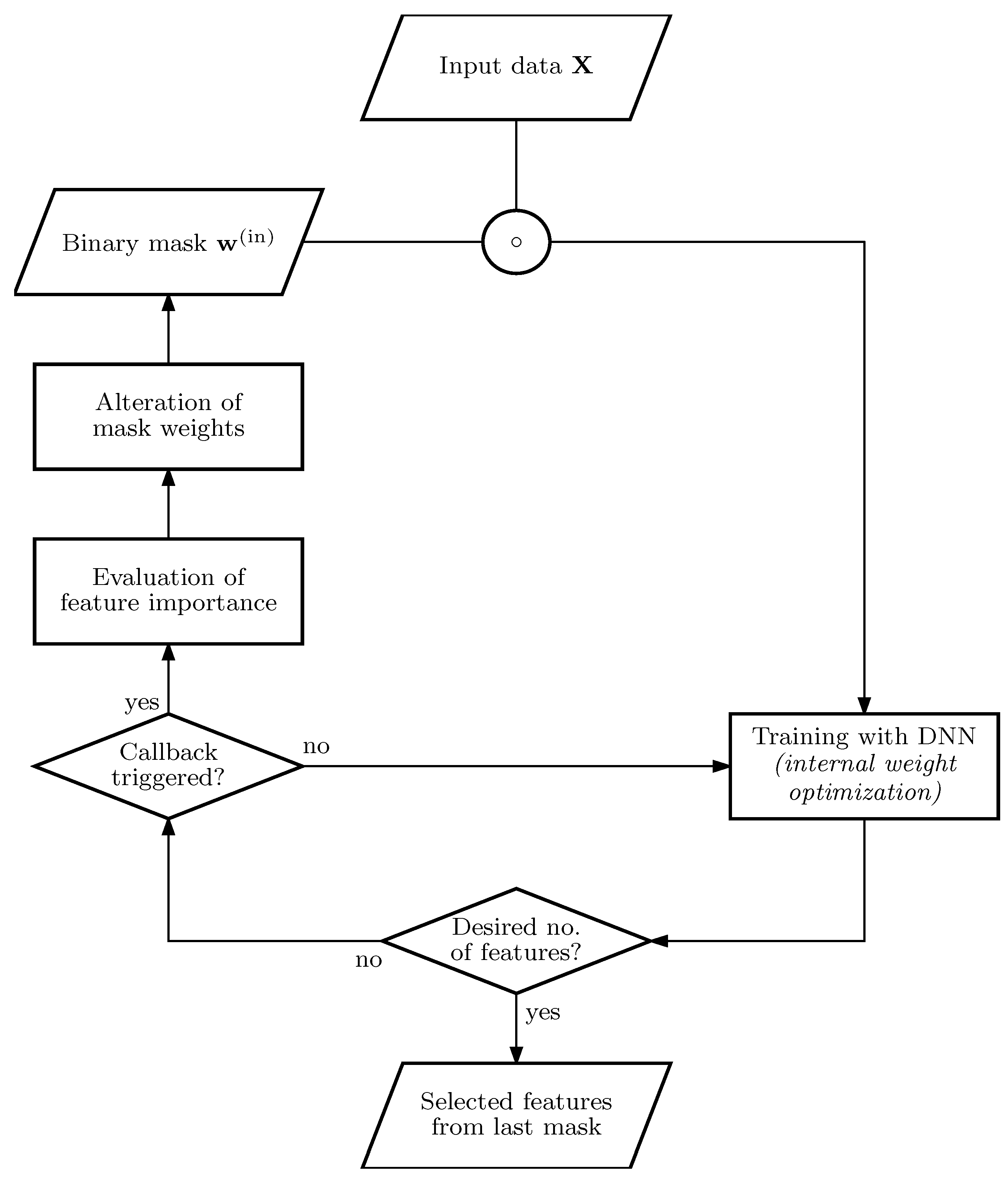
The crucial issue in such embedded approaches lies in the communication of the FS algorithm and the classifier. Inspired by the RFE from [21] and the recent approaches of [28], we make use of recursive and sequential pruning of feature nodes in the input layer. This recursivity is indicated by the loop structure in the process diagram of Figure 1.

At the start of the algorithm, the complete dataset $\mathbf{X}\in {\mathbb{R}}^{p\times n}$ with p features and n samples is considered and transferred to the classifier input unmanipulated, i.e., the binary mask ${\mathbf{w}}_{\mathrm{in}}\in {\mathbb{R}}^{p\times 1}=\mathbf{1}$. We use a deep neural network (DNN) as a classifier due to its inherent nonlinear properties. Its training process is executed within the lower loop in the process diagram. When the performance of the classifier is satisfyingly reliable and the callback is triggered, the algorithm exits the lower loop and enters the upper evaluation part. In this part, the importance of each feature is evaluated and a distinct proportion of the most informative features is selected. All of the others are pruned and neglected in ensuing optimization loops. This is done by altering the weights of the binary mask ${\mathbf{w}}^{\left(\mathrm{in}\right)}$. Subsequently, the DNN has to adapt to the increased difficulty of using sparser information. Everything is recursively repeated until either the desired number of features has been obtained or the classification accuracy drops beneath a given threshold and is unable to recover despite ongoing optimization.

The output of the algorithm is the last mask evaluated during the training, and a classifier is already pre-trained for the masked input. The outline and implementation of the proposed algorithm are split into the following two components: the classifier and the feature selection algorithm.

3.1. Classification with Deep Neural Networks

To prove the functionality in a general sense, we implemented a standard DNN consisting of one input $l_{\mathrm{in}}$, one output $l_{\mathrm{out}}$, and multiple hidden layers $l_i$. For the standalone classifier, only fully connected (FC, i.e., dense) layers were applied. In the forward pass of FC-type architectures, the output state vector

$${\mathbf{x}}^{\left(l\right)}=\varphi \left({\mathbf{Wx}}^{(l-1)}+\mathbf{b}\right)=\varphi \left(\mathbf{u}\right)$$

(11)

is calculated by multiplying the previous layer’s state vector ${\mathbf{x}}^{(l-1)}$ with a randomly initiated weight matrix $\mathbf{W}$ and then adding a bias vector $\mathbf{b}$. This bias vector is implemented to enable even more flexibility by shifting the input data. The weights and biases are trainable parameters. Afterwards, an activation function $\varphi$ is applied on the resulting $\mathbf{u}$ vector. As previously mentioned, this activation function is what makes the neural network a nonlinear classifier and provides advantages compared with linear transformations. An application of any arbitrary function is possible. 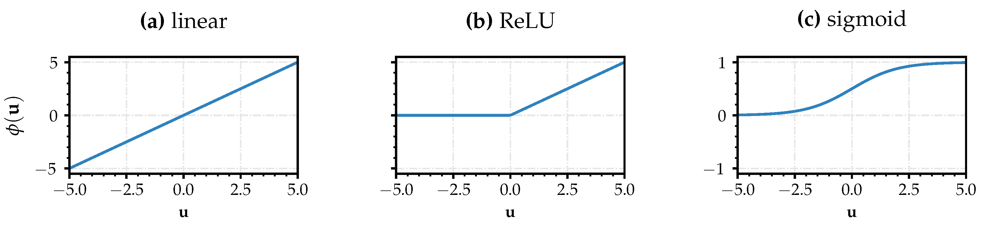The only restriction is the piece-wise differentiability of the function such that the back-propagation [29] algorithm is exercisable. We made use of the rectified linear unit (ReLU) function

$$\varphi \left(\mathbf{u}\right)=\max (\mathbf{0},\mathbf{u}),$$

(12)

which is a commonly used activation function that has been shown to deliver good results in fully connected architectures. Other typically used functions are tanh or sigmoid functions. The sigmoid function together with ReLU can be seen in Figure 2b,c. The linear function in Figure 2a represents a pseudo-activation within PCAs or LDAs after the transformation induced by the loadings in Equation (3) instead of the weight matrix $\mathbf{W}$.

In our proposed models, we use a feed-forward structure in which the number of nodes $n^{\left(l\right)}$ in each layer decreases as we go deeper into the neural network. Since FeaSel-Net is embedded into classifiers, the number of output nodes $n^{\left(\mathrm{out}\right)}$ has to correspond to the number of classes $n_c$. Unlike in the intermediate layers, the activation function used to compute the class prediction in the output layer $l_{\mathrm{out}}$ is the softmax function

$$\mathbf{y}=\varphi \left(\mathbf{u}\right)=\frac{e^{\mathbf{u}}}{{\sum }_{i=1}^{n_c}{e}^{\mathbf{u}}}$$

(13)

which causes the output vector $\mathbf{y}\in {\mathbb{R}}^{n_{\mathrm{c}}}$ to resemble probabilities. The output with the highest probability represents the predicted class. To train the network, we create the ground-truth target vector $\widehat{\mathbf{y}}$ via one-hot encoding and use the sparse categorical cross-entropy (CE) loss function

$$H(\mathbf{X},\mathbf{y})=-\sum _{\mathbf{x}\in \mathbf{X}}\widehat{\mathbf{y}}\left(\mathbf{x}\right)·\log \mathbf{y}\left(\mathbf{x}\right).$$

(14)

This loss is minimized by using the Adam optimizer [30].

Achieving an embedded feature selection algorithm is a rather challenging task, since it is not possible to alter the network architecture during the training process. Once the network is instantiated, its numbers of inputs, parameters, and layers are fixed; however, it is necessary to manipulate these to prune the input layer. To do so, we implemented a new embedded feature selection algorithm in the existing Keras and TensorFlow framework.

3.2. Feature Selection Callback

The communication behavior of the FS algorithm and the neural network is induced by implementing an appropriate and specifically constructed callback within the model. Usually, callbacks are used to log evaluation metrics, such as loss and accuracy values, or to preclude early stopping. In general, they provide the possibility to interact with the deep learning algorithm and adjust several parameters during the training at different entry points, such as at the end of an epoch or batch. The callback developed in this paper has the ability to assess the importance of input nodes and to prune nodes that are irrelevant by manipulating the weights of an upstream mask layer. The individual steps of the callback are explained in more detail below.

3.2.1. Implementation of the Callback Using Binarized Masking Layers

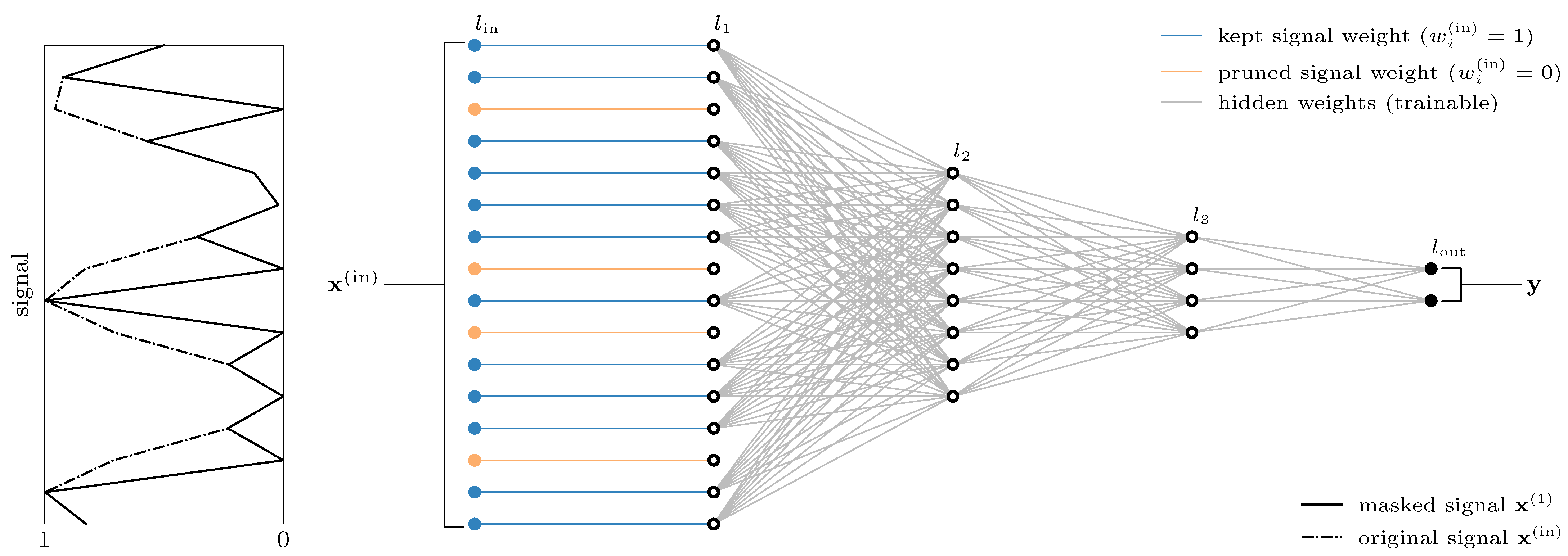
Section 3.1 described a standard fully connected multi-layer architecture for classification tasks, which we slightly adapted to attain the ability to mask the original signal according to Figure 1. This adapted architecture is shown in Figure 3.

We introduce a new and simplistic but effective layer that is able to constrain the input signal with a binarized weight vector ${\mathbf{w}}^{\left(\mathrm{in}\right)}\in [0,1]p\times 1$ . In our implementation, the layer type is called the LinearPass layer. Its output

$${\mathbf{x}}^{\left(1\right)}={\mathbf{w}}^{\left(\mathrm{in}\right)}\circ {\mathbf{x}}^{\left(\mathrm{in}\right)}$$

(15)

is the masked input for the actual neural network.

We deliberately do not want any parameters to be trained and initially set all weights ${\mathbf{w}}^{\left(\mathrm{in}\right)}=\mathbf{1}$ to obtain an unmasked and unmanipulated signal. The connections in Figure 3 will be set to zero if the corresponding feature is not found to be important. This happens whenever the callback is triggered. Manipulations of the bias vectors are not provided.

3.2.2. Callback Triggers

Standard callbacks are triggered every training epoch, and they log the loss and accuracy values for the training dataset ${}_{\mathrm{tr}}\mathbf{X}$ and validation dataset ${}_{\mathrm{v}}\mathbf{X}$. We utilize these recurring logged values to assess the performance of our model at each epoch e and query two trigger conditions:

(a)

Threshold criterion:

The loss gradient or accuracy values surpass a pre-defined threshold $\tau$.

(b)

Consistency criterion:

The threshold is surpassed for a minimal number of consecutive epochs $\Delta e_{\min }$.

When the logged values reach the threshold $\tau$, an internal counter starts. Only when the threshold criterion is continuously satisfied for $\Delta e_{\min }$ are the features pruned according to their importance. The evaluation itself is described in Section 3.2.3 and Section 3.2.4.

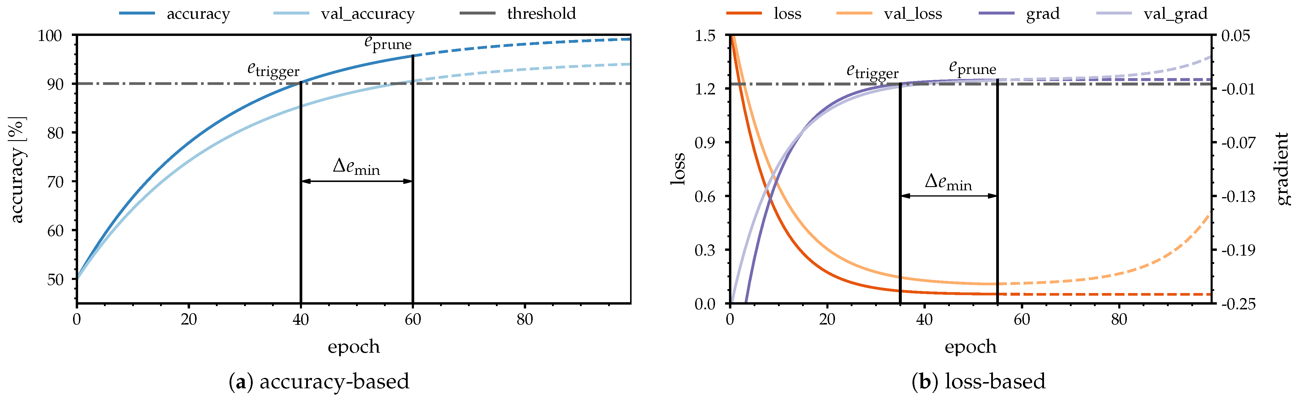
The trigger process for the accuracy-based feature selection is shown in Figure 4a. At epoch $e=40$, when the accuracy threshold value of ${\tau }_{\mathrm{a}}=90\%$ is surpassed for the first time, the pruning process starts with a delay of 20 epochs at $e=60$. Assuming that the accuracy value decreases and falls below the threshold again, the count for the consistency criterion is reset. Figure 4b analogously illustrates the loss-based trigger behavior.

Since different datasets and metrics rarely provide similar quantitative results, the algorithm utilizes the gradient of the current loss values. Here, the pruning process is triggered when the decline of the loss becomes stagnant. The low loss gradient threshold of ${\tau }_{\mathrm{g}}=0.005$ yields a pruning precisely at the moment of training stagnation. Thereby, we suspect that pruning at the moment of optimization stagnation will prevent over-fitting of the data. Hence, a potential increase in the validation loss, as indicated by the dashed line, is avoided.

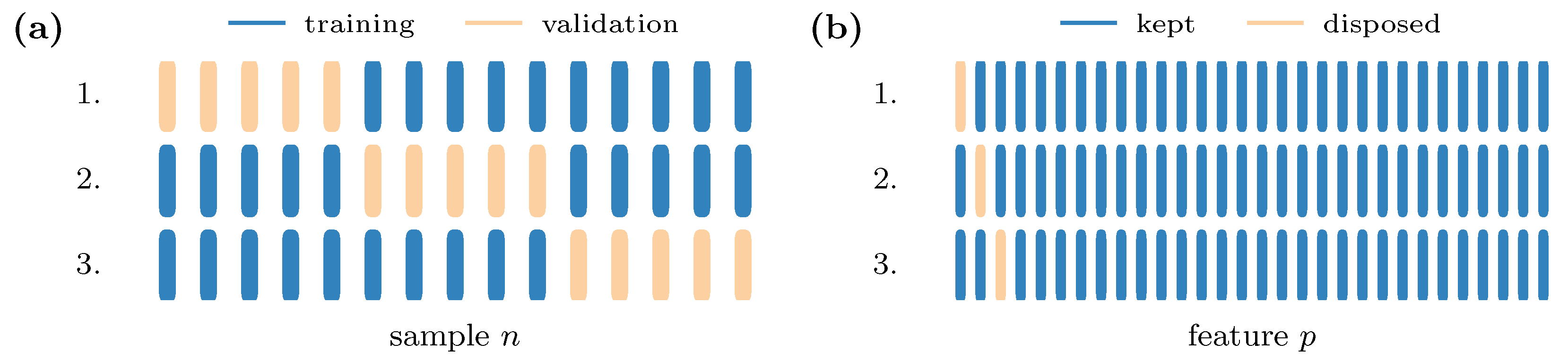
3.2.3. Creating an Evaluation Subset

At first, an evaluation dataset ${}_{\mathrm{e}}\mathbf{X}$ has to be generated, and it is appropriated for an isolated view of each feature node. To do so, we make use of the leave-one-out cross-validation (LOOCV) [2], an extreme variation of the k-fold cross-validation where $k=1$. The typical usage of the cross-validation is the k-time alternation of training and validation samples and the choice of the best-performing composition. Figure 5a shows this type of validation exemplarily for a small fictional dataset. Since we are interested in the importance of features rather than samples, we implement the LOOCV in combination with the disposal of one feature alternating at each iteration step; see Figure 5b.

Mathematically, this mask-like behavior can be expressed using a bit-wise inverted identity matrix:

$$\mathbf{M}=\mathbf{J}-\mathbf{I}$$

(16)

where $\mathbf{I}$ is an identity matrix and $\mathbf{J}$ is a matrix of ones with the size $p\times p$. We can now apply a mapping function $g:{\mathbb{R}}^{p\times n}\mapsto {\mathbb{R}}^{p\times n·p}$ to generate a p-time replication of the same training data ${}_{\mathrm{tr}}\mathbf{X}$, where exactly one feature is masked in each replication. The resulting evaluation data,

$${}_{\mathrm{e}}\mathbf{X}=\left[\begin{array}{cccc}{}_{\mathrm{tr}}{x}_{00}{m}_{00}& {}_{\mathrm{tr}}{x}_{01}{m}_{01}& \cdots & {}_{\mathrm{tr}}{x}_{0p}{m}_{0p}\\ {}_{\mathrm{tr}}{x}_{10}{m}_{00}& {}_{\mathrm{tr}}{x}_{11}{m}_{01}& \cdots & {}_{\mathrm{tr}}{x}_{1p}{m}_{0p}\\ ⋮& ⋮& \ddots & ⋮\\ {}_{\mathrm{tr}}{x}_{n0}{m}_{00}& {}_{\mathrm{tr}}{x}_{n1}{m}_{01}& \cdots & {}_{\mathrm{tr}}{x}_{np}{m}_{0p}\\ ⋮& ⋮& & ⋮\\ {}_{\mathrm{tr}}{x}_{00}{m}_{p0}& {}_{\mathrm{tr}}{x}_{01}{m}_{p1}& \cdots & {}_{\mathrm{tr}}{x}_{0p}{m}_{pp}\\ {}_{\mathrm{tr}}{x}_{10}{m}_{p0}& {}_{\mathrm{tr}}{x}_{11}{m}_{p1}& \cdots & {}_{\mathrm{tr}}{x}_{1p}{m}_{pp}\\ ⋮& ⋮& \ddots & ⋮\\ {}_{\mathrm{tr}}{x}_{n0}{m}_{p0}& {}_{\mathrm{tr}}{x}_{n1}{m}_{p1}& \cdots & {}_{\mathrm{tr}}{x}_{np}{m}_{pp}\end{array}\right],$$

(17)

are then tested, and the impact of the masked features is evaluated with respect to the test loss. In case a vast number of samples and features leads to an enormous amount of data, we provide a possibility to use only a subset of the training data as evaluation data, which would have an equal size for all classes. To further accelerate the evaluation process, already masked features are not regarded in the mapping of Equation (16), and each of its new rows

$${\mathbf{m}}_i:={\mathbf{m}}_i·w_i^{\left(\mathrm{in}\right)}$$

(18)

is deleted if $w_i^{\left(\mathrm{in}\right)}$ has already been set to zero. To prevent buffer overflows in huge datasets, especially at the beginning of the algorithm when $\mathbf{M}$ is still complete, the mapped data are split into batches ${}_{\mathrm{e}}{\mathbf{X}}_f$, where each batch represents one feature f.

3.2.4. Evaluation of Feature Importance

Within the callback, the training process is paused and the significance of the masked features is evaluated. Therefore, the same loss function as during the training process (Equation (14)) is also used for the evaluation, but in contrast to the training, the losses are not averaged over the complete epoch or its batches, but rather over each feature masking the dataset. This is done because the interest lies in the deterioration of discriminability due to these missing features. Alternatively, one can look at this behavior as dividing the set into one batch per feature, where the losses of each batch are averaged. These considerations yield another new metric based on Equation (14), which we call feature omission impact (FOI):

$${\mathcal{I}}_f\left({}_{\mathrm{e}}{\mathbf{X}}_f,\mathbf{y}\right)=H_f\left({}_{\mathrm{e}}{\mathbf{X}}_f,\mathbf{y}\right).$$

(19)

At this point, it has to be clarified that previously pruned features are not evaluated by not mapping them in Equation (17), because they inherently cannot provide any information to the classifier.

3.2.5. Feature Pruning

Since the negative influence of masked input nodes on the classification performance is evaluated, the view for interpreting the resulting entropy values has to be changed. While the entropy should normally be minimized to achieve unambiguous predictions, we now keep the features f that resulted in the highest FOI and the biggest differences in the results of unmasked prediction. The weights

$${\mathbf{w}}_i^{\left(\mathrm{in}\right)}\left[\mathrm{argsort}\left(\mathcal{I}\right)\right]=0\forall 0<i\le n_{\mathrm{p}}\in \mathbb{R}$$

(20)

of the masking LinearPass layer are manipulated by sorting the features according to their information richness from the lowest to the highest and setting the least informative features’ weights to zero. The pruning number $n_{\mathrm{p}}$ defines how many entries are pruned. Some datasets have many features, and pruning one feature after another is tremendously time-consuming. Thus, the algorithm offers two possibilities for setting the pruning number. It is either set once for the linear pruning method or it is constantly re-calculated for the exponential decrease in information depending on the pruning rate $\pi$. After the pruning, the optimization process is resumed with the masked input ${}_{\mathrm{e}}\mathbf{X}\left({\mathbf{w}}^{\left(\mathrm{in}\right)}\right)$. As soon as the consistency and threshold criteria are met again, the recursive binary mask is obtained using the adapted evaluation set ${}_{\mathrm{e}}\mathbf{X}\left({\mathbf{w}}^{\left(\mathrm{in}\right)}\right)$ as the input for the next pruning step in Equation (19).

The sorting algorithm for the the indices i in ${\mathbf{w}}^{\left(\mathrm{in}\right)}$ is defined by

$$\mathrm{argsort}{\left(\mathbf{x}\right)}_i:=\left|\{j\in \{1,\cdots ,n\}|\left(x_j<x_i\right)\}\right|,$$

(21)

and it sorts the features from the lowest to the highest ${\mathcal{I}}_f$.

Eventually, the feature selection process is finished when one of the following criteria is met:

(a)

Success criterion:

The number of leftover features $n_{\mathrm{e}}$ reaches the desired number of features q.

(b)

Non-convergence criterion:

The threshold is not reached within a given number of epochs $\Delta e_{\max }$.

4. Results

We apply the proposed method on the Wine Classification dataset provided by [22] to demonstrate the performance of the FeaSel algorithm and compare it with the linear methods described in Section 2, as well as the XGBoost algorithm and the nonlinear stochastic gates (STG) method. This multivariate dataset is broadly used in ML research and covers LDA and PCA investigations [31,32], as well as fully connected neural network approaches [33]. Despite being multivariate, it is still small enough to gain an overview on what happens during the algorithm’s execution. The dataset consists of $n_{\mathrm{s}}=178$ samples divided into $n_{\mathrm{c}}=3$ classes of almost equal set size. The original number of features is $p=13$. Since the feature values are partially of greatly different magnitudes (e.g., alcohol compared to proline), a standardization of the values for each feature according to Equation (6) is necessary. Additionally, we assure the correct dimensionality for a fully connected neural network and use a training–testing split of 80%, with which we obtain the dimensionalities given in

Table 1. Dataset size, dimensionality, and number of samples per class.

Dataset (i)	Data ${}_{\mathbf{i}}\mathbf{X}$	Targets ${}_{\mathbf{i}}\mathbf{y}$	Samples per Class
Training $\left(\mathrm{tr}\right)$	$[142,13]$	$[142,3]$	[45–57–40]
Validation $\left(\mathrm{v}\right)$	$[36,13]$	$[36,3]$	[14–14–8]
Evaluation $\left(\mathrm{e}\right)$	$\mathrm{tr}\left(\mathbf{M}\right)·{}_{\mathrm{tr}}\mathbf{X}$	$\mathrm{tr}\left(\mathbf{M}\right)·{}_{\mathrm{tr}}\mathbf{y}$
Test $\left(\mathrm{te}\right)$	$[178,13]$	$[178,3]$	[59–71–48]

. These subsets are used for either of our FS methods. The evaluation dataset dimensionality is a multiplication of the training dataset with the trace of the mask matrix $\mathrm{tr}\left(\mathbf{M}\right)$. A consistent dataset for all methods is obtained by using the same random seed for all training–testing splits.

4.1. Feature Selection with PCA

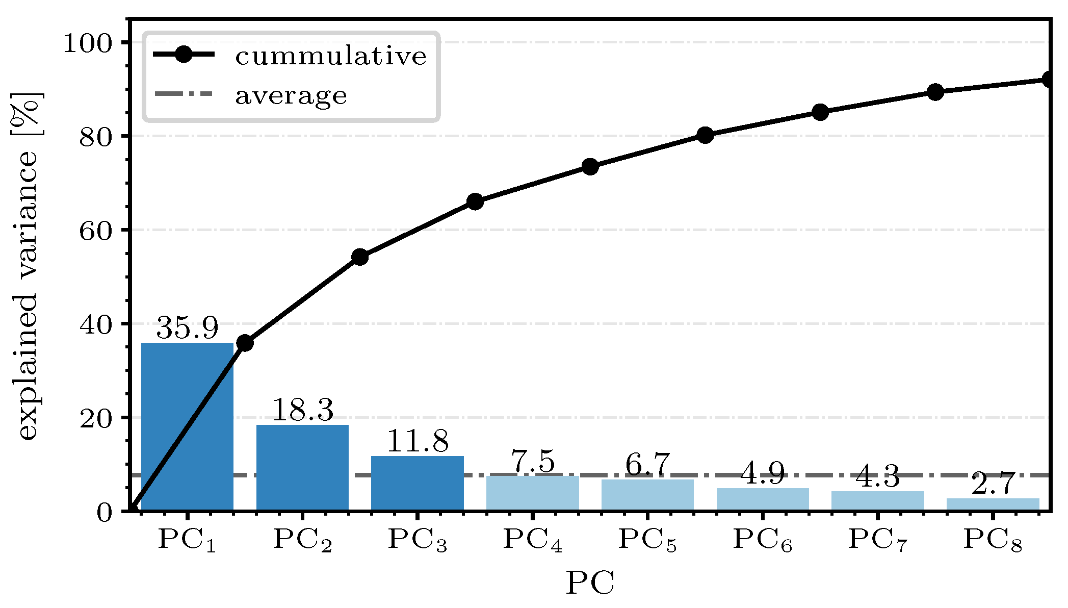
The PCA loadings for the training subset are calculated according to the steps described in Section 2.1. Figure 6 shows the scree plot for the first eight components of PCA for the Wine Classification dataset. Since a distinct elbow—an elbow is a subjective criterion for the decision on whether to include components in the transformation and is characterized by a strong kink in the scree plot [34]—was not observed in the plot, the average explained variance with $7.7\%$ was chosen as the threshold. Components with a variance lower than this threshold were not regarded. Thus, we narrowed down the transformation to the first three components, which made up $66.0\%$ of our data’s information.

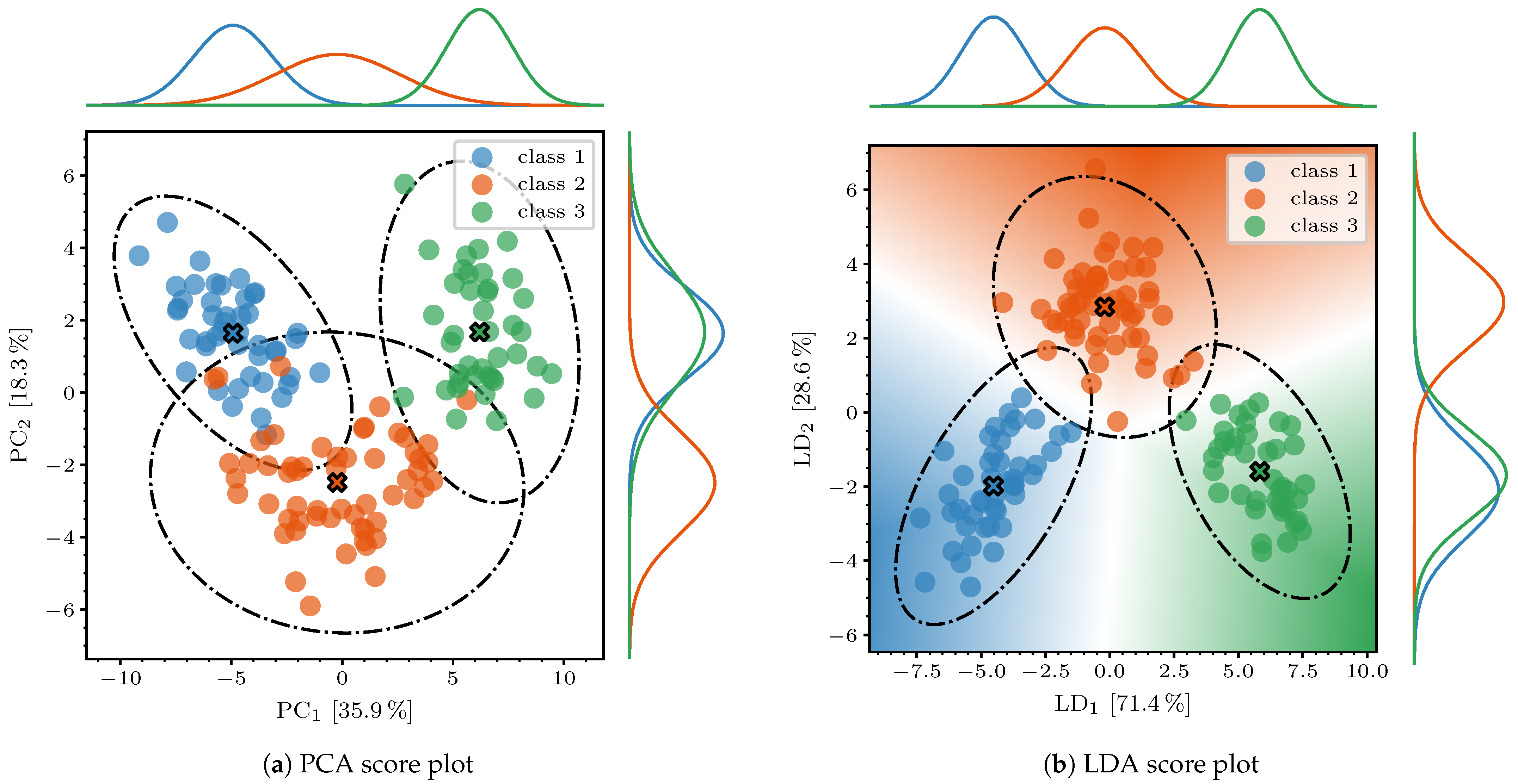
The resulting score in Figure 7a looks promising in terms of separating the classes when considering the latent space defined by the first two components only. Although there are a few intersections and overlaps, we can clearly observe a class separation. This capability breaks down when considering the third component in combination with one of those mentioned before. Hence, we confine ourselves to the interpretation of the loadings in the first two components. 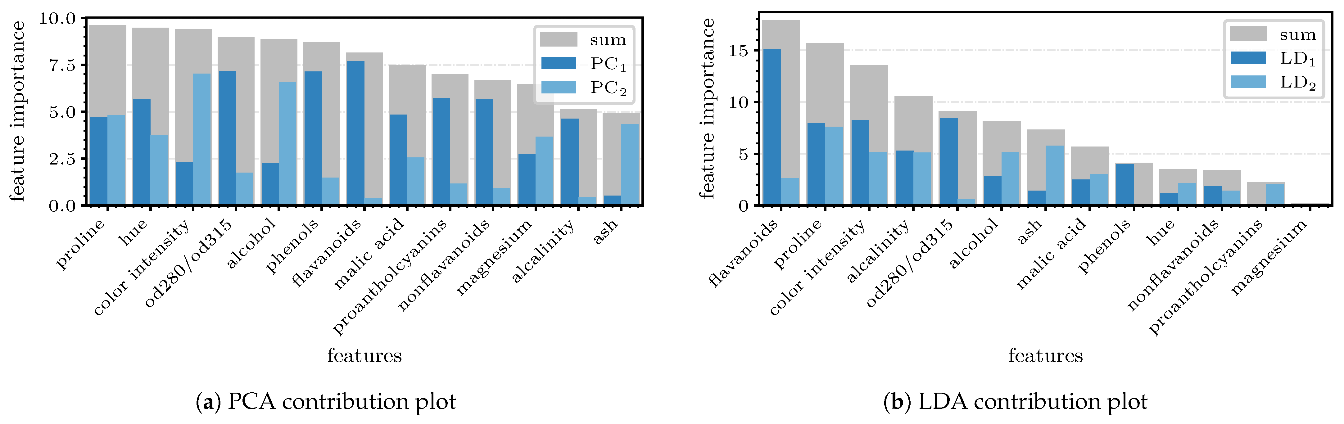Figure 8a shows the contribution of each feature to the specific PC. The evaluation and, thus, the sorting of the feature importance is done according to [24], where the feature contribution is calculated by applying Equation (7) on the q most important eigenvectors $\mathbf{V}$ along the feature axis. Since we want to include the components’ explained variance in our consideration, we use the scaled loadings $\mathbf{A}$ instead. For the examined dataset, we set $q=2$ due to the previous considerations. The features are distilled by choosing the first three features in Figure 8a (proline, hue, and color intensity) as the most prominent, but there is only a modest difference from their successors.

4.2. Feature Selection with LDA

The same research group from [24] also showed the applicability of this feature evaluation method with LDA [35]. We have already discussed the additional class information that this transformation type offers and can clearly see an improvement in the separation in Figure 7b. It is even possible to completely separate the clusters for the training set. When looking at the decision boundaries in this score plot, there is no training sample point that has been misclassified. Furthermore, the projected normal distribution of the orange class 2 cluster clearly shows the influence of the LDA objective—the transformation wants to minimize the variances within the classes. Although the distribution in the score plot of Figure 7a and, especially, the projection of ${\mathrm{PC}}_1$ is flat and wide, it is almost circular and narrower in the LDA score plot; see Figure 7b. Because of this distinctiveness and the fact that ${\mathrm{PC}}_1$ and ${\mathrm{PC}}_2$ together explain $100\%$ of the data, we are allowed to investigate only these components again. Just like before, the most important features are extracted from the contribution plot in Figure 8b, where a concise difference in the results can be seen. With the help of LDA, it is found that flavanoids seem to be much more relevant than hue, which had the third lowest contribution, unlike in the PCA, where it achieved the second highest. Nevertheless, there is a consensus on the importance of proline and color intensity. Another conspicuity is the noticeably increased variance in ${\mathsf{\sigma }}_{\mathrm{LDA}}=5.18\%$ in the contribution compared to that for PCA (${\mathsf{\sigma }}_{\mathrm{PCA}}=1.54\%$). Altogether, these findings lead to an unambiguous tendency in which LDA will perform better in terms of feature selection.

4.3. Feature Selection Using Feasel-Net

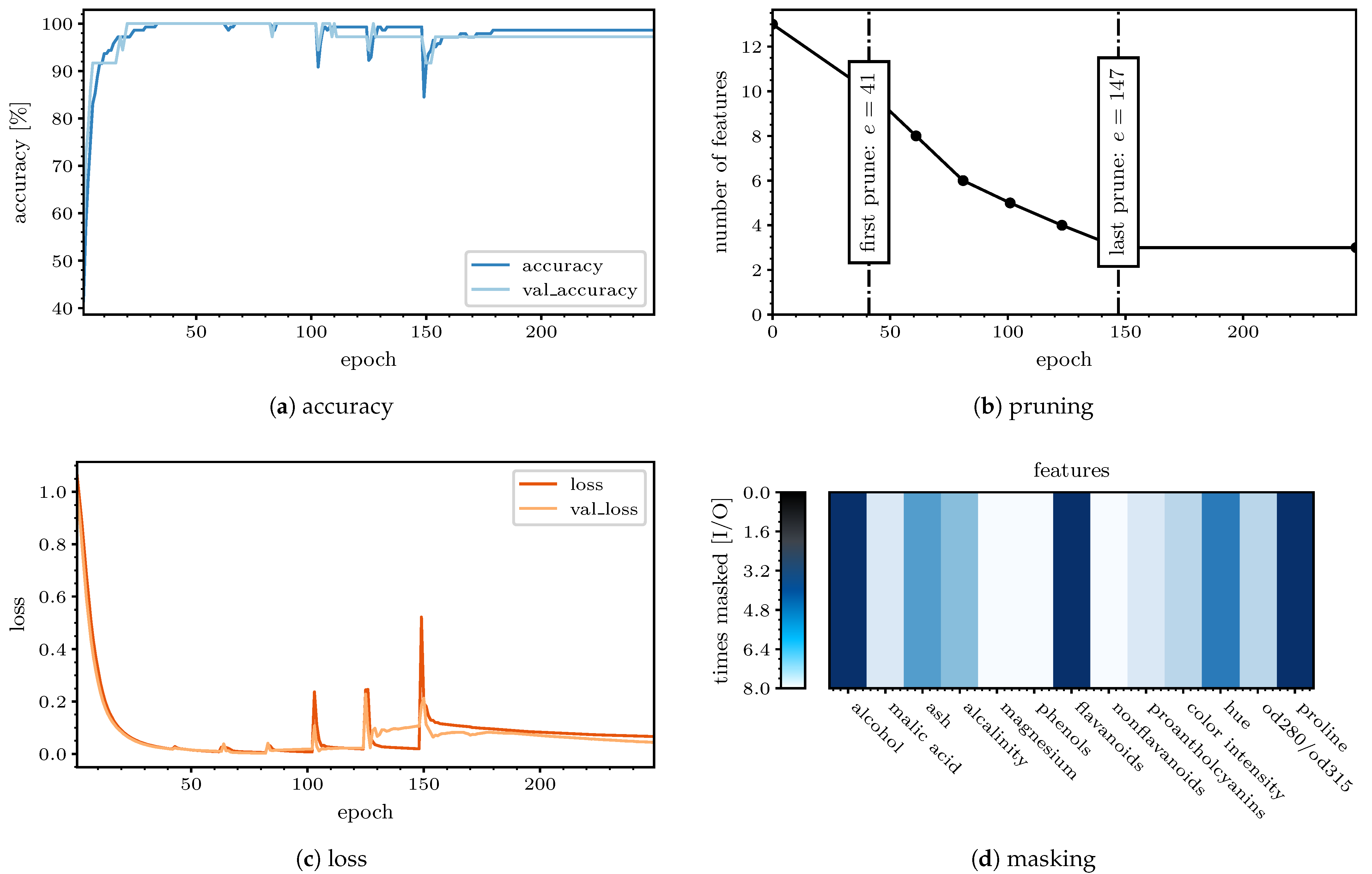
When using the same data with the newly proposed FS algorithm, we can clearly observe the recursiveness throughout the model’s optimization process, as shown in Figure 9a,c. After 21 epochs, the accuracy value surpasses the threshold for the first time, and $\Delta e=20$ epochs later, we can observe the first pruning, where magnesium, phenols, and nonflavanoids have been deleted. 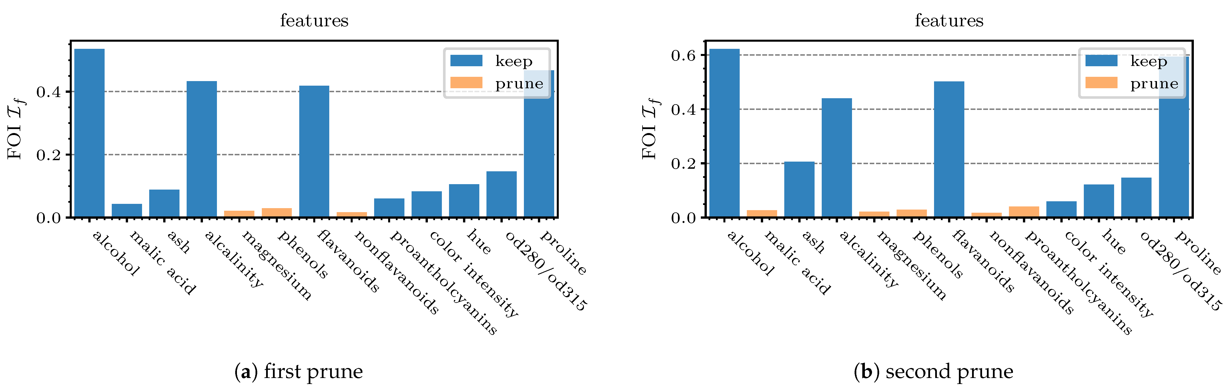A drop in the classification accuracy cannot be perceived at either $e=41$ or 20 epochs later, which is when the second pruning happens, with malic acid and proantholcyanins being deleted. The FOIs at these first two pruning steps are shown in Figure 10a,b. Since the training is continued with quasi pre-trained weights after each pruning, the model recovers quickly. The most prominent drop is observed at the last pruning epoch at $e=147$, which is self-evident due to the further decreasing amount of information. When reaching $q=3$ parameters, the algorithm stops the training process after $\Delta e_{\max }=100$ more epochs to optimize the discrimination one last time with the selected features. Outstandingly high values of $99.1\%$ were achieved for the training accuracy and $97.6\%$ for the validation accuracy, even though the input nodes were reduced to these three aforementioned features and the information was compressed to $\kappa =23.1\%$. The exact number of features at each pruning epoch can be retrieved from Figure 9b. By the end of the FeaSel-Net application, the three selected features were flavanoids, proline, and alcohol. Figure 9d shows the pruning history in terms of how often a feature was masked throughout the FS process. 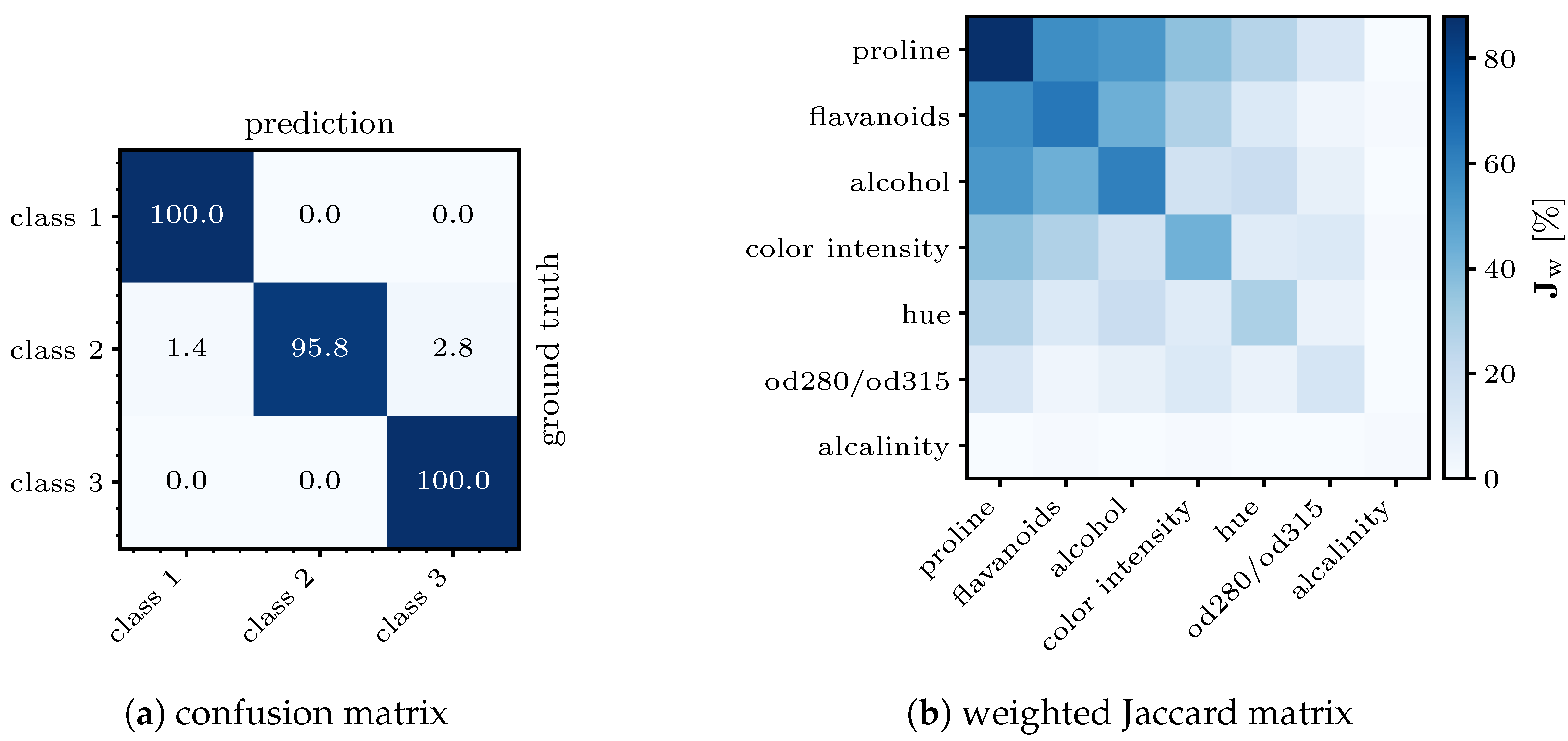Features such as magnesium were considered to be the least important and were masked since the very first pruning step, whereas hue showed the darkest color and was, hence, the most important apart from the chosen features. This coincides with the findings from the PCA and LDA methods. The confusion matrix in Figure 11a shows perfect sensitivity for class 1 and class 3 and is satisfactory for the other class. Altogether, an average sensitivity of $\mathrm{SEN}=98.6\%$ was achieved. In terms of classification accuracy and specificity, the results were of an even higher magnitude, with $\mathrm{ACC}=98.8\%$ and $\mathrm{SPE}=99.2\%$.

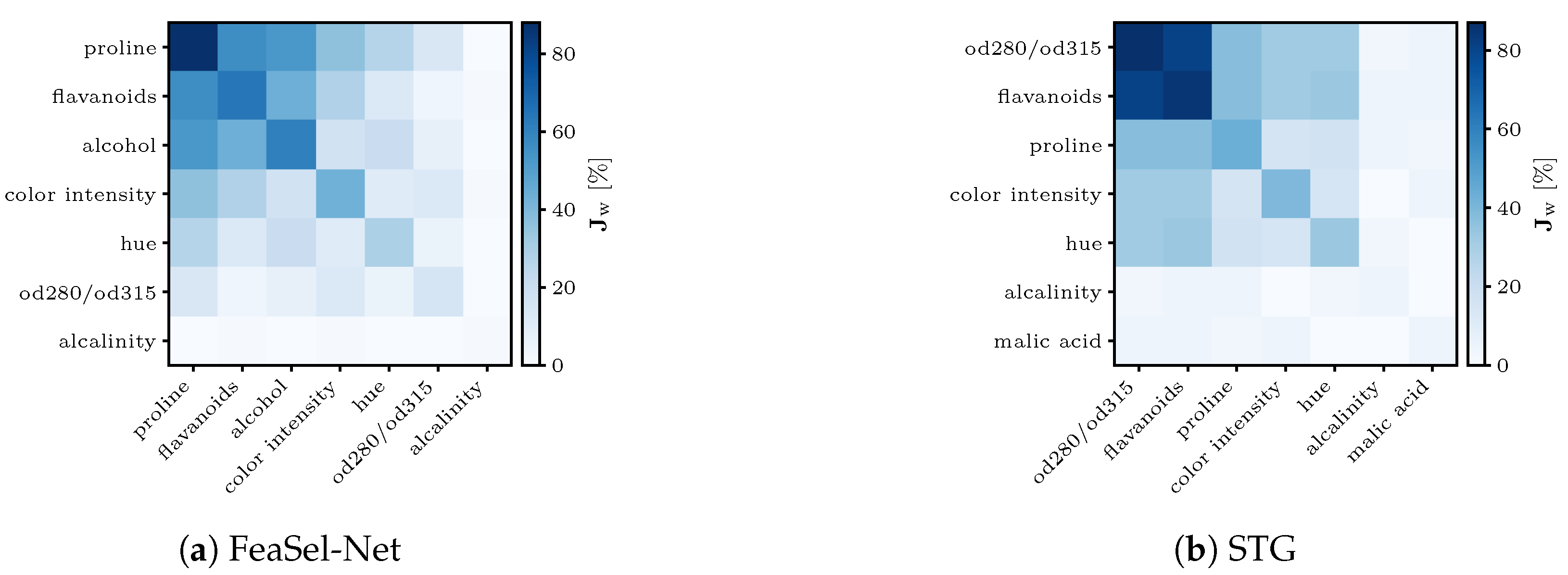
Since the weights of fully connected layers in neural networks are randomly initialized, volatility in the extracted features has to be expected, e.g., by using the uniformly distributed values according to Glorot [36]. Therefore, 100 executions or runs $n_{\mathrm{r}}$ of FeaSel applications are statistically evaluated to prove the consistency and the extent of this fluctuation. In order to assess the probability of finding the most relevant features and to analyze the inter-dependencies among them, a weighted Jaccard matrix ${\mathbf{J}}_{\mathrm{w}}$ is introduced in Appendix A.1. The diagonal in Figure 11b can be interpreted as a normalized histogram for the selected features. Furthermore, the matrix directly implies that the features retrieved from the elaborated execution discussed before (proline, flavanoids, and alcohol) were also chosen the most often, with percentages of 87.7–60.8% of all runs. It additionally shows that these three features were commonly picked together, and in the case that some other feature was picked, it was most likely selected together with the prolines, which emphasized the importance of this attribute. Alkalinity was the last feature to be displayed, since every other feature was not chosen at all. Hence, these can be neglected in good conscience. The other features that were determined by linear transformations (color intensity and hue) occurred in the fourth and fifth positions, respectively.

4.4. Comparison of Different Feature Selection Methods

All three previously analyzed methods yielded slightly different sets of features that were distilled after the selection. To validate the performance of each selection method, a classification using only the masked dataset was executed. We also compared it to the features chosen with the tree-based XGBoost algorithm [13] and a recent approach with the so-called stochastic gates (STG), where the FS was already embedded as a regularizer into a deep-learning-based classifier. The regularizing hyperparameter $\lambda$ had an immense effect on the number of leftover features. It was set to $0.3$ such that an average number of $2.9$ selected features was achieved. Further information on this method can be found in [17]. Since the STGs was embedded into neural networks, there was much randomness. Similarly to the FeaSel-Net approach, we applied it several times and calculated its weighted Jaccard matrix. The certainty of selections using STGs was found to be lower than FeaSel-Net’s, which is shown in Appendix A.3. Additionally, a random FS with alcohol, alkalinity, and color intensity is included in

Table 2. Selected features from all analyzed FS methods.

Method	Feature 1	Feature 2	Feature 3
PCA	proline	hue	color intensity
LDA	flavanoids	proline	color intensity
XGBoost	flavanoids	proline	color intensity
STG	od280/od315	proline	flavanoids
random	alcohol	alkalinity	color intensity
FeaSel-Net	proline	flavanoids	alcohol

to demonstrate the importance of choosing features accurately. Even though only one (alkalinity) out of these three randomly selected features was not found to be important by the investigated FS methods, it still performed clearly worse.

In order to compare the effectiveness of the feature selection methods, another fully connected neural network was implemented that accepted only three input values (i.e., the masked signal). We purposefully chose only three features to ensure variations among each selected feature set on the one hand, as well as, on the other, to use as little information as possible in order to clearly show differences between each FS method. It output a probability vector corresponding to the three classes; see

Table A3. Different model architectures used for the Wine Classification dataset. The table shows the number of nodes in each layer and the number of parameters.

Model Type	${\mathit{l}}_{\mathbf{in}}$	${\mathit{l}}_{\mathbf{LP}}$	${\mathit{l}}_1$	${\mathit{l}}_2$	${\mathit{l}}_3$	${\mathit{l}}_{\mathbf{out}}$	Params
FeaSel-Net	13	13	13	8	5	3	370
Reduced	3	-	6	12	6	3	207
Unmasked	13	-	9	4	3	3	193

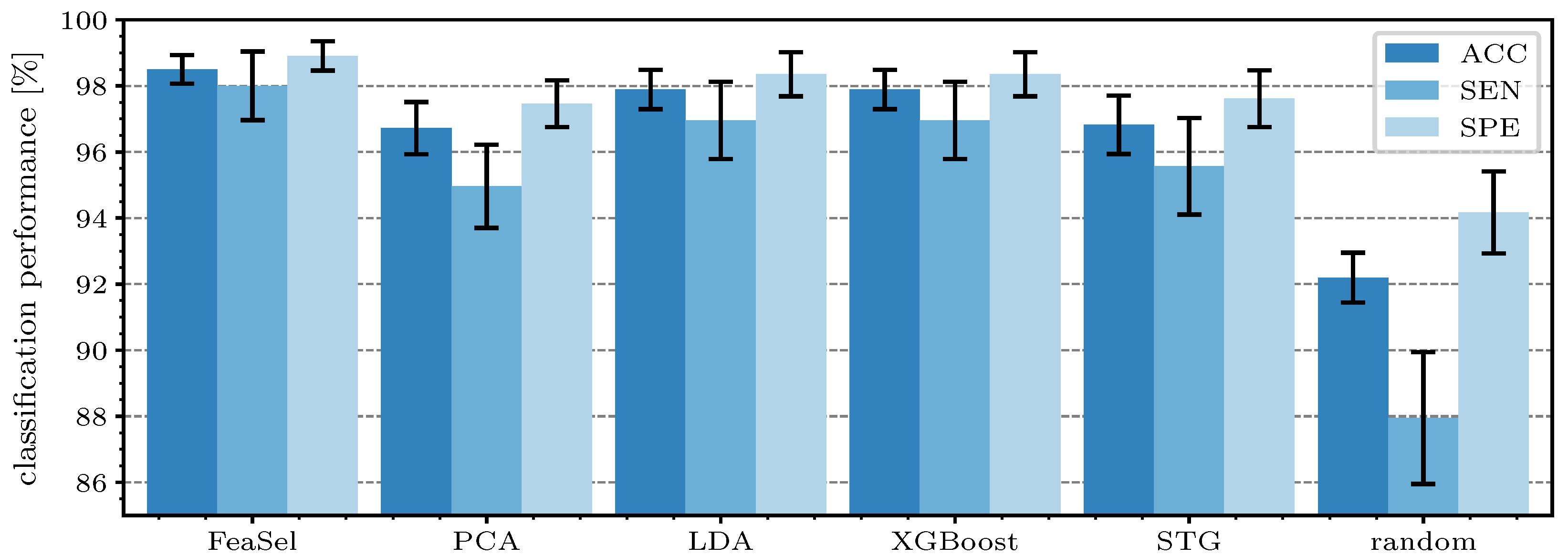
. A fair comparison of the discriminability was ensured by using the exact same model with the same hyper-parameters for all methods. The only variation was given by the input signal, which was chosen according to Table 2. The model was, parameter-wise, distinctly smaller than the classifier network used in Section 4.3. It was trained 25 times, and the average and standard deviation for accuracy (ACC), sensitivity (SEN), and specificity (SPE) were calculated. Outliers from PCA, LDA, and XGBoost optimizations were removed in the evaluation. Figure 12 shows the performance parameters for each retrieved feature mask. The overall accuracy of the classification using the features from FeaSel-Net amounted to $\mathrm{ACC}=98.50\pm 0.43\%$, which was an increase of $0.6\%$ compared to the second-best result (LDA and XGBoost) and even $1.8\%$ higher than the PCA benchmark, whereas $\mathrm{SPE}=98.91\pm 0.44\%$ also improved at the same level. When looking at $\mathrm{SEN}=98.0\pm 1.04\%$, an increase of $1.1\%$ compared to the LDA and $3.2\%$ compared to PCA method was achieved. Using the features that were retrieved by using the STG, the results were only slightly better than the PCA-derived selection. On average, the superior FeaSel-Net approach had a $6.8\%$ higher accuracy, a distinctly improved sensitivity with $11.5\%$, and a $5.0\%$ better specificity than that obtained when using randomly chosen features.

4.5. Generalizability of Masked Data

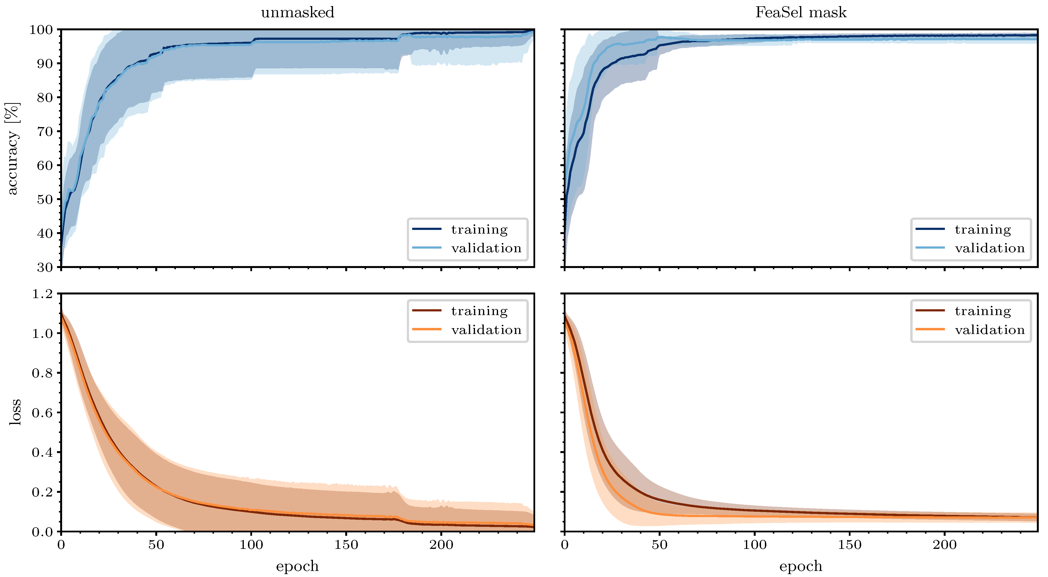
FeaSel-Net was specifically developed to use less input information and still provide reasonable classification results without dramatic drops in the performance. To investigate the improvements due to the preceding feature selection, we compared the results of training histories from 25 unmasked and masked optimizations of the Wine Classification dataset over 250 epochs, as shown in Figure 13. The network used for the masked data was the same reduced classifier as in Section 4.4, and for the unmasked set, an architecture with a similar number of trainable parameters and network depth was used to provide the same optimization potential; see Table A3. Two outlier runs were removed from the unmasked and one from the masked dataset. FeaSel-Net’s average accuracy after 250 epochs of training with only three input features accounted for ${\mathrm{ACC}}_{\mathrm{Wine}}=98.1\%$ compared to $99.4\%$ with the unmasked set. On the other hand, its validation accuracy’s variance averaged over all epochs $e>50$ amounted to $\pm 1.12\%$ and was more than eight times smaller than the unmasked averaged variance of $\pm 8.91\%$. An average validation accuracy of more than $95.0\%$ was achieved in epoch $e=24$ already, and the maximum value accounted for $97.8\%$. The unmasked dataset unsurprisingly achieved better overall classification results with $99.2\%$ instead, but it had to be trained 40 epochs longer until $95.0\%$ was reached. We could not identify an over-fitting during training in either dataset, since a small number of parameters and, thus, a modest complexity were used for the model. When comparing these results, it can be seen that a significantly faster convergence was obtained, and the variance was significantly smaller when masking the data according to the FeaSel-Net findings beforehand. Both observations are indicators for a better generalizability. The smaller variance in the masked optimizations proves a steady and reliable finding of the global minimum.

4.6. Investigation of Different Datasets

In this section, an analysis of other datasets from [22] that confirm the potential of FeaSel-Net as an alternative for the feature selection of 1D data is undertaken. With the (feature-wise) very small Iris [37], medium-sized Mice Protein Expression (MPE) [38], and extremely large Arcene datasets [39], we want to tackle data attributed with different levels of complexity. The parameters specified for each FeaSel-Net run in the following are based on the settings for the Wine Classification set; see

Table A2. Specified values for the FeaSel-Net building parameters.

Parameter	Symbol	Value
Build
compression rate	$\kappa$	None
leave-one-out cross-validation	−	True
number of features	q	3
number of features to prune per step	$n_{\mathrm{p}}$	None
number of samples	$n_{\mathrm{s}}$	None
pruning rate	$\pi$	$0.2$
pruning type	−	exponential
Trigger
decay	$\delta$	0.0
maximal number of epochs	$\Delta e_{\max }$	100
minimal number of epochs	$\Delta e_{\min }$	20
threshold (accuracy-based)	${\tau }_{\mathrm{a}}$	$0.98$
threshold (loss-based)	${\tau }_{\mathrm{g}}$	None
type	−	accuracy
Evaluation
accelerate	−	False
decision metric	−	average
metric	−	cross-entropy
normalization	−	min-max
rationalize	−	False
remove outliers	−	True
scale	−	False

. Changes in the parameters will be mentioned explicitly.

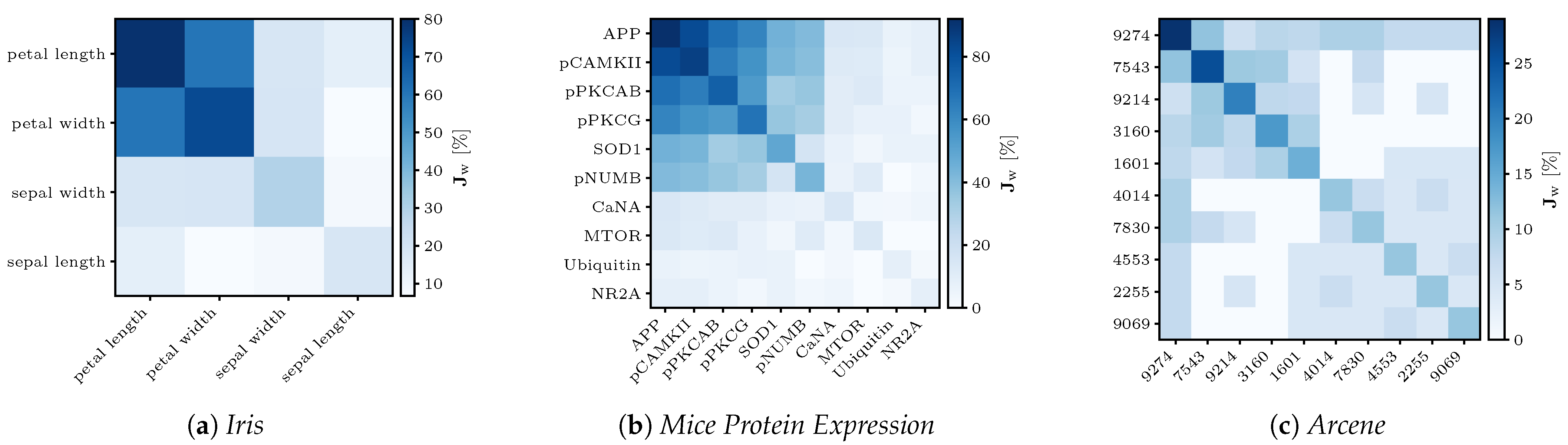
4.6.1. Iris

The Iris dataset consists of samples with only four attributes and is separated into three classes. According to Fisher’s findings in [37], the attributes of petal length and petal width contribute the most information to a discrimination between the three classes. In his work, he originally introduced an earlier version of the LDA and found that the petal attributes’ coefficients for the transformation were roughly 1.5–4.5 times higher and, thus, more important than the sepal attributes. With the FeaSel-Net method, we found the exact same attributes to be more relevant. The petal length was chosen in $79.4\%$ and petal width in $72.5\%$ of all runs; see Figure A1a. Because of the minute number of attributes, a desired number of features of $q=2$ was specified, with which a compression ratio of $\kappa =50\%$ was achieved.

4.6.2. Mouse Protein Expression

The authors of [38] originally investigated protein levels in mice exposed to contextual fear conditioning. They used self organizing maps (SOM), an unsupervised clustering technique, to identify biologically important differences in medication-induced protein levels of healthy mice and mice with trisomy 21. Feature selection with FeaSel-Net achieved even better results on this medium-sized dataset with $p=77$ features. In $92\%$ of all cases, the protein APP was chosen to be the most important feature followed by pCAMKII with $86\%$. A distinct cluster of the first six proteins can be noticed in Figure A1b. All proteins found in this Jaccard matrix were also found to be important discriminants for generating the SOMs. Since the number of samples was 5–$10\times$ larger compared to the numbers in the other datasets, a batch size of 64 instead of 16 was specified. With $q=3$ set for the algorithm, a compression ratio of $\kappa =3.9\%$ was obtained, and it resulted in a classification accuracy of approximately ${\mathrm{ACC}}_{\mathrm{MPE}}=85.4\%$.

4.6.3. Arcene

This particularly large dataset with $p=10\mathrm{k}$ features was part of the NIPS 2003 feature selection challenge. With the application of FeaSel-Net on this dataset, we wanted to focus on the computability of such large datasets. When looking at the results, less distinctive feature importance distributions were obtained in the Jaccard matrix of Figure A1c. While the matrices of the Iris and MPE sets looked structured and some attributes were considerably more important than others, selection in the Arcene dataset yielded sparser and more chaotic results. However, the feature at position 9274 still seemed to be very important, since it was chosen more than every fourth time in a highly compressing setting with $q=10$ features left and a compression rate of $\kappa =0.1\%$. In 35 executions, this was more than 250 times as often as that when choosing the features completely randomly. It was also seemingly dominant because it was the only attribute that was chosen in combination with every other attribute depicted in the Jaccard matrix at least once. On average, the classification with the reduced input yielded a ${\mathrm{ACC}}_{\mathrm{Arcene}}=94.3\%$ classification accuracy. An overview of all datasets is given in

Table 3. Overview of the compression of the input using FeaSel-Net and the resulting classification performance after 250 epochs of training with only three input features.

Dataset ${}_{\mathbf{te}}\mathbf{X}$	Features p	Features q	Compress. $\mathit{\kappa }$	$\mathbf{ACC}$ [%]	FS $\mathbf{ACC}$ [%]
Iris	4	2	$50.0$	$98.6\pm 0.1$	$92.7\pm 9.0$
Wine Classification	13	3	$23.1$	$99.5\pm 1.7$	$98.1\pm 0.5$
MPE	77	3	$3.9$	$96.4\pm 9.6$	$87.1\pm 3.8$
Arcene	10,000	10	$0.1$	$96.8\pm 0.5$	$94.3\pm 0.2$

.

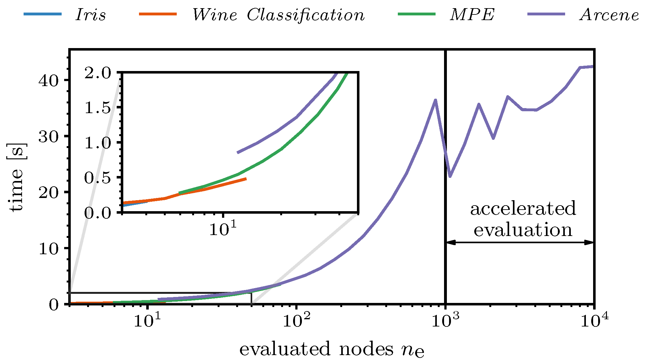
4.7. Computation Time

Finally, the computation time of the proposed FeaSel-Net was examined for all of the previously introduced datasets. For this benchmark test, we used cuDNN, a GPU-accelerated library that is usable within the TensorFlow environment, and Accelerated Linear Algebra (XLA) compilation was enabled. The hardware consisted of an RTX 2070 SUPER GPU and an AMD Ryzen 5 2600X CPU. As described in Section 3.2.3, nodes that were pruned prior to the current pruning epoch were not evaluated. This linearly accelerated the evaluation process, as can be seen in Figure 14. In the logarithmically scaled plot, a linear increase in the time with the number of evaluated nodes can be perceived until $n_{\mathrm{e}}$ reached 1000. The kink at this position was due to an acceleration of the evaluation, where the evaluation set was divided into a maximum number of $n_{\mathrm{b}}=1000$ batches. For the Arcene dataset, the batch size became $n_{\mathrm{b}}=10$, i.e., ten adjacent features were evaluated at the same time. This yielded an almost constant duration of approximately $40\mathrm{s}$ for the evaluation of datasets with $n_{\mathrm{e}}>1000$. The zig-zag behavior was induced by ensuring natural numbers as batch sizes and, consequently, varying numbers of batches. When reaching, e.g., $n_{\mathrm{e}}=6400$, seven adjacent features were considered simultaneously; therefore, $n_{\mathrm{b}}=915$ batches were generated. Looking at smaller numbers of evaluated features (detailed view; $n_{\mathrm{e}}<50$), there was a noticeable jump of nearly half a second between the Arcene dataset and the MPE dataset, which occurred because of the larger neural network architectures during the FS process.

The overall computation time of FeaSel-Net amounted to $16.85\pm 2.04\mathrm{s}$ when averaged over 25 executions. Compared to the $22.42\pm 0.17\mathrm{s}$ of the STG method, a slight improvement of the computation time was obtained. This was mainly due to the early stopping criteria implemented in FeaSel-Net. All linear methods need less than a second for their computation. Compared to linear methods, feature selection with neural network approaches generally takes a lot of time. In particular, when the amount of data increases, the difference will be very noticeable. Thus, there is a trade-off between computation time and finding the best features.

5. Conclusions

In this work, we introduced FeaSel-Net, a feature selection algorithm that can easily be embedded in any fully connected neural network classifier. With its novel concept of recursively pruning the information in the input layer of the network, it forces the classifier to constantly adapt to the repeated omission of information such that the discrimination ability of the classifier remains at a supreme level. The evaluation of the feature omission impact is done by applying the leave-one-out cross-validation along the feature axis and assessing the impact of the missing feature on the classification result.

By comparing the outcome of FeaSel-Net when applied on the popular Wine Classification dataset with those of traditionally used linear approaches (PCA, LDA, and XGBoost), it was proven that the inherent nonlinear transformations in FeaSel-Net were beneficial. Another comparison with the current stochastic gates method showed that regularizer-based feature selection strongly depends on initialization and that recursive pruning methods such as FeaSel-Net select with a higher certainty. A classification executed in connection with each analyzed feature selection method with a dataset reduced to the specific features led to the best results when using FeaSel-Net’s findings. In a different experiment in which the training process of unmasked data was juxtaposed with one with pre-selected features, it was confirmed that the algorithm could be a remedy against the curse of dimensionality. The application of FeaSel-Net to three more datasets of extremely contrasting sizes—from only four and up to 10k features—underlined that it covered several different use cases.

Applications of FeaSel-Net in other domains, such as physics, automotive development, or even the financial sector, are possible. However, the motivation for developing this algorithm originated from the field of spectroscopy and the urge to find new potential biomarkers that recent statistical approaches cannot reveal. With a sparser input and selective regions of interest in the spectral domain, spectrometer scans can be executed faster and measurement systems can be specifically engineered for the specific tasks. In fact, an article in which FeaSel-Net was applied on the Raman spectra of tumorous bladder tissue has already been published [40].

Even though the application of the algorithm is restricted to 1D datasets so far, it also has the potential to be used to prune uninformative filters—for example, in image processing. In order to analyze this potential, FeaSel-Net needs to be implemented in convolutional neural networks in future works.