Article

Micro- and Macro-Scale Topology Optimization of Multi-Material Functionally Graded Lattice Structures

by
Jerónimo Santos
1,
Abdolrasoul Sohouli
2 and
Afzal Suleman
1,2,*
1
Instituto de Engenharia Mecânica (IDMEC), Instituto Superior Técnico, Universidade de Lisboa, 1049-001 Lisboa, Portugal
2
Department of Mechanical Engineering, University of Victoria, Victoria, BC V8W 2Y2, Canada
*
Author to whom correspondence should be addressed.
J. Compos. Sci. 2024, 8(4), 124; https://doi.org/10.3390/jcs8040124
Submission received: 3 March 2024 / Revised: 19 March 2024 / Accepted: 25 March 2024 / Published: 28 March 2024
(This article belongs to the Special Issue Characterization and Modelling of Composites, Volume III)

Abstract

:
Lattice structures are becoming an increasingly attractive design approach for the most diverse engineering applications. This increase in popularity is mainly due to their high specific strength and stiffness, considerable heat dissipation, and relatively light weight, among many other advantages. Additive manufacturing techniques have made it possible to achieve greater flexibility and resolution, enabling more complex and better-performing lattice structures. Unrestricted material unit cell designs are often associated with high computational power and connectivity problems, and highly restricted lattice unit cell designs may not reach the optimal desired properties despite their lower computational cost. This work focuses on increasing the flexibility of a restricted unit cell design while achieving a lower computational cost. It is based on a two-scale concurrent optimization of the lattice structure, which involves simultaneously optimizing the topology at both the macro- and micro-scales to achieve an optimal topology. To ensure a continuous optimization approach, surrogate models are used to define material and geometrical properties. The elasticity tensors for a lattice unit cell are obtained using an energy-based homogenization method combined with voxelization. A multi-variable parameterization of the material unit cell is defined to allow for the synthesis of functionally graded lattice structures.

1. Introduction

Engineers across a variety of industries, including aerospace, automotive, and biomedical, have long sought lightweight yet high-efficiency structures, such as those with high stiffness, high specific strength, or good heat dissipation properties [1,2]. One approach to achieving these properties is through numerical topology optimization, which gained widespread attention following the publication of the seminal work by Bendsøe and Kikuchi in 1988 [3].
It is important to investigate the potential benefits and drawbacks of using different geometries at the micro-scale and evaluate the applicability of the methodology as proposed by Wang et al. [4]. In order to minimize computational complexity and reduce processing time, a voxelization method is suggested as a viable alternative to a highly discretized conformal mesh for constructing the continuous surrogate model that represents the graded evolution of the unit cells.
A lattice structure consists of an arrangement of struts or faces connected by nodes, which when assembled builds up to a geometry within a determined unit cell. Connecting these unit cells results in a complete lattice structure. Lattice structures are comparable to other materials, such as foam or honeycomb types of material. The research community has disseminated works which indicate that lattice structures have better mechanical properties in compression and shear compared to foams and honeycombs [5,6,7]. The enhanced mechanical properties are mainly due to the fact that lattice structures can be tailor-made for each desired application. The unit cells or the struts/faces within the unit cell can have different design variables assigned to them, enabling numerous combinations of the geometry in use and optimization of them to satisfy specific requirements.
Topology optimization is a process used to find the optimal material distribution that satisfies one or more objective functions while adhering to a set of constraints and boundary conditions. The design domain is discretized into several finite elements in a finite element approach and the material distribution is controlled and described by one or more design variables, where the simplest case assumes the density of the finite element to be the only design variable.
Topology optimization can achieve optimal structures by considering geometric patterns that transform spatially over the defined design domain and through multiple length-scales. When a single scale is considered for optimization, it is classified as mono-scale, while when more than one scale is considered it is categorized as multi-scale. Multi-scale approaches can optimize both material micro-structure and structural macro-scale concurrently, providing better results than approaches performed separately and/or successively.
Homogenization theories form the basis of multi-scale approaches, allowing for the computation of effective material properties by considering the material to be made up of repeating patterns of similar unit cells. The review paper by Wu et al. [8] categorizes unit cell topology design approaches into five major categories. The more flexible the design is, the more problems may arise concerning connectivity, integrity, and manufacturing issues.
Multi-scale optimization has been the focus of many research works, including those that employ a single-design variable parameterization. Wang et al. [9] and Watts et al. [10] successfully employed surrogate models to represent the elasticity tensor characterizing the material properties in 2D and 3D unit cell optimizations, respectively. Ypsilantis et al. [11] extended this approach to multimaterial 3D optimization of the micro-scale. Nguyen and Choi explored the effect of increasing design flexibility by optimizing the unit cell build orientation and addressing the concept of equivalent unit cells for conformal lattice designs [12].
In more recent works, multi-variable multi-scale optimization has also been studied. Imediegwu et al. [13] analyzed a multi-variable parameterization of the unit cell using 7 design variables, which has been expanded to 10 design variables in a recent work by the same group [14]. However, the high number of design variables in such models leads to highly complex computational models that may require a dynamic database that updates during the optimization process to reduce computational effort and time.
A previous work by Costa et al. [15] presented a method that enabled (in short) the discretization of unit cell geometries at the micro-scale and the study of its mechanical capabilities at a macro-scale level. Taking the aforementioned works into consideration, the present work focuses on the discretizion and study of different geometries, while also presenting four distinct case studies from the literature to be used in the macro-scale part of the process.

2. Theoretical Background

2.1. Topology Optimization

Topology optimization (TO) is a process that aims to find the optimal distribution of one or more materials within a given design domain while considering a set of constraints, such as volume fraction. An optimization problem can be formulated to minimize the compliance of a material subject to a volume constraint, which can be represented by Equation (1).
In this equation, c refers to compliance, | Ω | ( ρ ) represents the volume of material, U is the displacement vector, and F is the global force vector [16].
Find : ρ = { ρ 1 , , ρ N } , Minimize : c ( ρ ) = U T K U = e = 1 N u e T k e u e , subject to : | Ω | ( ρ ) / | Ω | Λ , : K U = F , : 0 ρ e 1 , e = 1 , , N .
The element stiffness matrix, k e , can be obtained by using the elasticity tensor, D, which can be determined for isotropic materials.
k e = Ω e B T DB d Ω e .
To compute the strain-displacement matrix, B, an isoparametric finite element formulation is used, where the physical coordinate system is transformed into a reference coordinate system centered in the element.
The expression in Equation (2) can be reformulated in terms of natural coordinates, as shown in Equation (3), where | J | denotes the determinant of the Jacobian matrix. To accurately calculate the element stiffness matrix, the computation of matrices B and J is critical. Gao et al. [17] explain the process for calculating these matrices in detail. Gaussian quadrature can be used to evaluate the integral in Equation (3), and it is considered more effective than the Newton–Cotes quadrature because it optimizes the position and weights of the sampling points at which the integral is evaluated.
k e = 1 1 1 1 1 1 B T DB | J | d ξ d η d ζ

2.1.1. Sensitivity Analysis

To solve a topology optimization problem, it is necessary to perform a sensitivity analysis, which involves calculating the derivatives of both the objective function, c ( ρ ) , and the volume constraint, | Ω | ( ρ ) (as defined in Equation (1)), with respect to the design variables.
By representing the global stiffness matrix as a sum of N element stiffness matrices, k e G , the formulation can be written in the global reference frame (Equation (4)), where u e is the element vector of nodal displacements.
t i a l c ( ρ ) t i a l ρ e = u e ( ρ ) T t i a l t i a l ρ e k e ( ρ e ) u e ( ρ )
The derivative of the volume constraint, | Ω | ( ρ ) , with respect to the density variable is given by Equation (5).
t i a l | Ω | ( ρ ) t i a l ρ e = | Ω e |

2.1.2. Filtering

Filtering techniques are commonly employed in the topology optimization (TO) process to mitigate numerical issues, such as checkerboard patterns and mesh dependency. Mesh-independent filtering methods are the most widely used despite other potential solutions, such as perimeter and global gradient control [18].
The modified element density, x e , is based on a neighboring region of that element, determined by the filter radius, r m i n [19]. The density of the finite element, e, is computed using Equation (6), where N e represents the set of neighboring elements to which the distance from centre to centre of the elements, Δ ( e , i ) , is smaller than the filter radius dimension, and H e i is a weight factor defined in Equation (7) [16].
x ˜ e = 1 i N e H e i i N e H e i x i
H e i = m a x ( 0 , r m i n Δ ( e , i ) )
However, the application of a density filter results in the loss of physical meaning for the original densities, x i , and the solution must rely on filtered densities. This approach produces filtered sensitivities, t i a l ψ ˜ t i a l x e , which can be mathematically expressed using Equation (8). A small value is incorporated into the equation to avoid division by zero when the element densities ρ e are zero.
t i a l ψ ˜ t i a l x e = 1 m a x ( γ , x e ) i N e H e i i N e H e i x i t i a l c t i a l x i

2.2. Material Homogenization

To simulate the mechanical behavior of a lattice material, a homogenization technique may be employed. This approach enables the determination of the effective elastic properties of a material, assuming two conditions hold: first, the macro-scale characteristics are much greater than the micro-scale dimensions (large separation of scales), and second, the micro-structure exhibits a periodic distribution on the macro-scale, composed of periodically repeating unit cells [20].
One can use a finite element approach which solves the equations using the finite element method. The periodic unit cell can be divided into N finite elements to write Equation (9). Superscript i pertains to the six independent test strains in a 3D scenario, while subscript e denotes the element domain. B e represents the element strain-displacement matrix and D e is the elasticity tensor for the typically isotropic material that makes up the corresponding finite element.
K χ i = f i , i = 1 , , 6
K = e = 1 N V e B e T D e B e d V e
f i = e = 1 N V e B e T D e ϵ 0 ( i ) d V e
Once the solution for the displacement field, χ i , is established, the term χ e i can be determined, and this can be achieved by solving Equation (9).
D i j H = 1 | V | e = 1 N u e A ( i ) T k e u e A ( j )
If the unit cell is subjected to an imposed strain field, ϵ i j 0 , the displacement field can be expressed, as shown in Equation (13) [21,22]. The fluctuation field term corresponds to a deviation from the linear displacement field that arises due to the heterogeneous structure of the composites.
For a continuous physical body assumption to be valid, two continuity conditions must be met at the boundaries of the repeating unit cells. The first condition is that the displacements must be continuous and the unit cell boundaries cannot overlap or separate from others of adjoined unit cells. Equation (13) ensures this condition.
χ i = ϵ i j 0 y j + χ i *
The second condition is that the traction distributions at the opposite parallel boundaries of a periodic unit cell must be the same. To address this, Equation (13) can be transformed into a set of explicit expressions that consider the displacements on pairs of parallel opposite surfaces of the unit cell. Equations (14) and (15) provide the general formulation for the displacements on a pair of parallel opposite surfaces, with the superscripts k + and k denoting the opposite parallel surfaces perpendicular to the kth = 1, 2, 3 principal direction (i.e., X, Y, or Z axis).
χ i k + = ϵ i j 0 y j k + + χ i *
χ i k = ϵ i j 0 y j k + χ i *
To eliminate the fluctuation term, χ i * , Equation (15) can be subtracted from Equation (14), resulting in Equation (16).
Even though Equation (16) guarantees the first continuity condition, known as the traction continuity, where the normal and shear stresses must be equal at parallel boundaries, it may not always be met. However, for a displacement-based finite element,
χ i k + χ i k = ϵ i j 0 ( y j k + y j k ) = ϵ i j 0 Δ y j k .

2.3. Lattice Structures

Depending on their individual properties, lattice structures can be categorized into two groups: stretch-dominated and bending-dominated lattices.
The choice between these two types of lattices depends on the application’s primary objective. In stretch-dominated lattices, M 0 , external loads are balanced by axial tension and compression in struts, meaning that no bending occurs at nodes, while in bending-dominated lattices there are too few struts to balance the external forces without balancing the moments induced at the nodes, causing bending stresses to develop in struts [23,24].
M = s 3 × j + 6 .
The Maxwell number measures the stiffness of the lattice structure by taking into account the number of struts, s, and joints, j, that make up the unique geometry of the unit cell (Equation (17)).

2.4. Sensitivity Analysis

In order for the optimizer to update the design variables and achieve convergence for the final solution, it requires access to the derivatives of both the objective function and the volume constraints with respect to those design variables. These sensitivities are crucial for the optimizer to make informed decisions about how to adjust the design variables. Specifically, the sensitivities regarding the objective function can be expressed in mathematical terms to provide a more precise understanding of the relationship between the design variables and the objective function, as expressed in Equation (18):
t i a l c ( X ) t i a l ρ ˜ e = u e ( X ) T t i a l k e ( ρ ˜ e , x ˜ m a t e ) t i a l ρ ˜ e u e ( X ) .

3. Methodology

3.1. Surrogate Model

The first step involves building a sampling-point database that includes various combinations of design variables, lattice branch radius, and the resulting homogenized elasticity tensor for each combination. The second step involves connecting all sampling points to create the continuous surrogate model, which requires selecting a suitable method to fit the data into a continuous model using regression analysis.
A voxel-based model is chosen to generate the discretization of the micro-scale. The unit cube geometry is divided into structured hexahedral finite elements with eight nodes per element, resulting in a highly regular mesh. This choice is based on the fact that the voxel-based discretization eases the definition of periodic boundary conditions that are pivotal to the adopted homogenization method [13].
To address this issue, Imediegwu et al. [13] proposed a scheme that considers the linear dependency between the material assigned to each voxel and the number of nodes inside the domain delimited by the lattice structure. If this distance is less than or equal to the radius, the node is considered active and counts to set the density to the elements that share it. If it is more than the radius, the node is considered inactive. Research papers such as [10,12,25] are examples of how voxelization has been used to compute effective material properties for different lattice structures.

3.1.1. Unit Cell Parameterization

The two-variable parameterization of the unit cell is accomplished using the relative density and aspect ratio as design variables. The relative density represents the percentage of solid material volume in each unit cell and is defined in Equation (19). The aspect ratio, ρ e x t , is defined as a ratio between the volume of external lattice branches, V e x t , and the total lattice material volume, V s t r u t , as presented in Equation (20).
ρ = V s t r u t V u c
ρ e x t = V e x t V s t r u t
Overall, the two-variable parameterization approach follows the rationale presented by Wang et al. [4], with only the variable names changing. The approach enables the concurrent optimization of both the macro- and micro-scale in a multi-scale topology optimization.

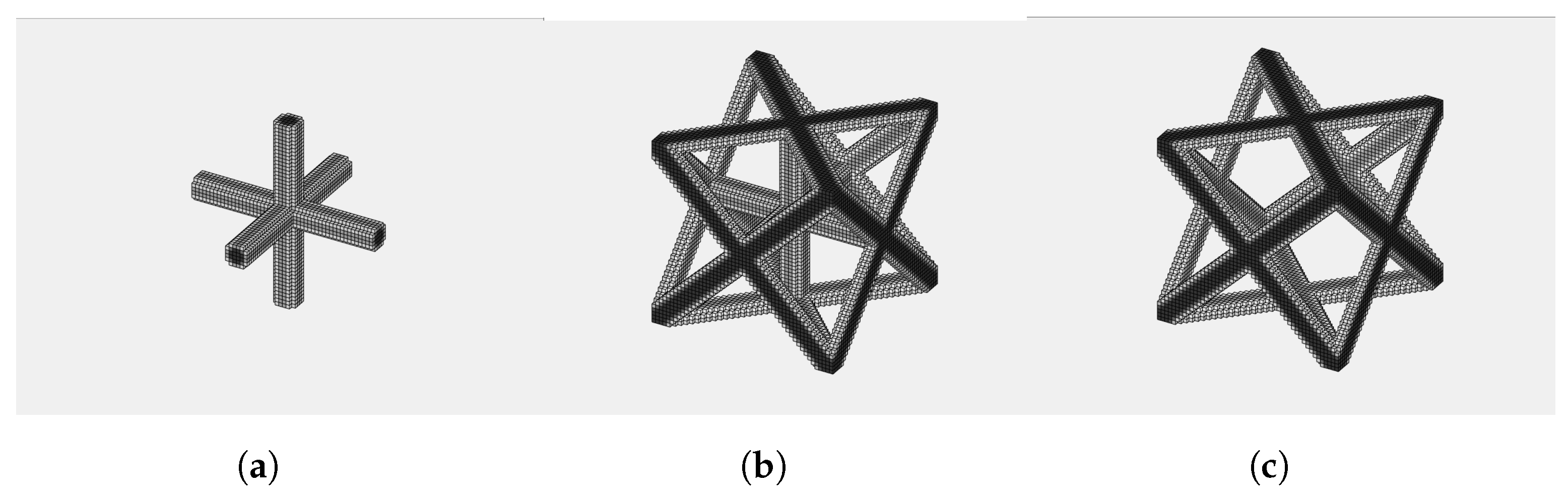
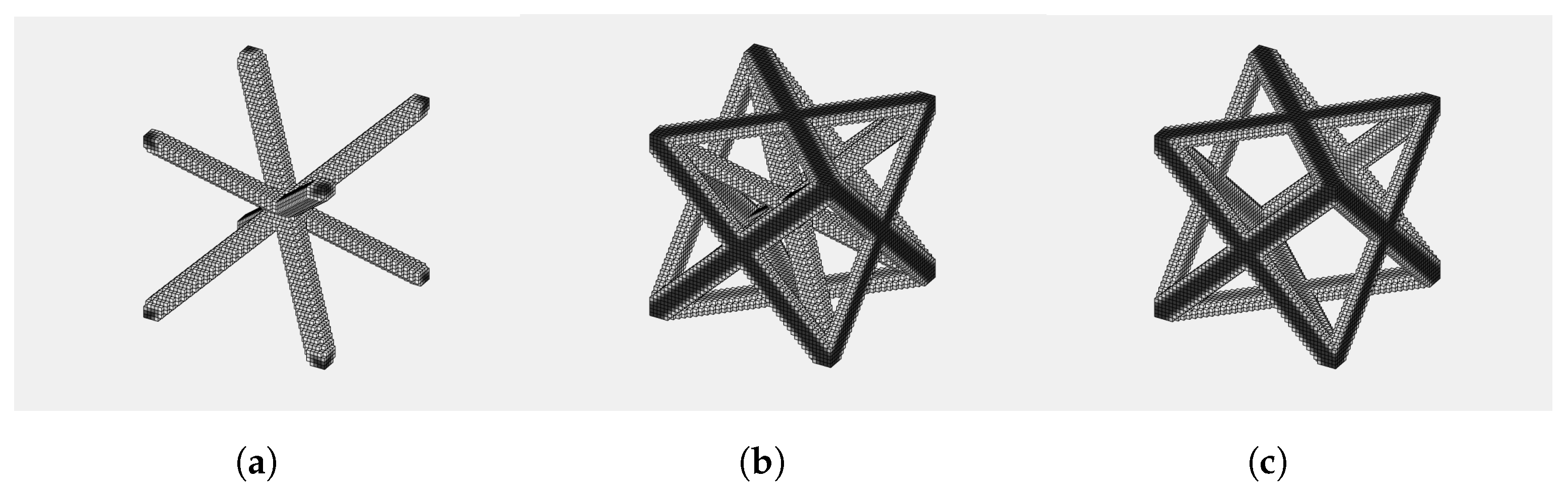
3.1.2. Unit Cell Geometries

The geometries used at a micro-scale level in each unit cell play a fundamental part when compiling and creating the study cases in the TO process, in the later stages of the work. As stated previously, six geometries are to be presented and studied at both micro- and macro-scale.
In the literature [5,26,27,28], there might be specific titles for such geometries/branches presented next, although (and to better identify the final geometry combination) in the context of this work these were the titles given. Each geometry is identified as the arbitrary name of the outer branches plus arbitrary name of the inner branches.
The geometry in Figure 1 has a Maxwell number of 12 and is therefore bending-dominated.
The geometry in Figure 2 has a Maxwell number of 1 and is bending-dominated.
The geometry in Figure 3 has a Maxwell number of 1 and is bending-dominated.
The geometry in Figure 4 has a Maxwell number of 0; therefore, it is stretch-dominated.
The geometry illustrated in Figure 5 has a Maxwell number is 9 , meaning this geometry is bending-dominated.
Lastly, the geometry in Figure 6 has a Maxwell number of 13 ; this geometry is bending-dominated.

3.1.3. Sampling Point Database

The assembling of a complete database is a crucial step in the development of a surrogate model. In this case, the range of relative densities of the sampling points varies from 0 to 1, initially with steps of 0.025 up to rel. density of 0.1, then steps of 0.1 until the value of 0.9 is reached, and finally steps of 0.025 until a value of 1 of relative density. The aspect ratio varies from 0 to 1 as well, with a constant step interval of 0.1. Thus, the database has a total of 165 sampling points that each have a unique combination of the two design variables, relative density and aspect ratio, leading to different lattice branch diameters for each sampling point. Once the sampling-point database script has collected all the required data, the points are connected together during the data-fitting process.

3.1.4. Regression Model

This approach aims to connect all the sampling points and can be visualized in a three-dimensional graph as a surface, considering a two-design variable parameterization of the lattice material unit cell. One of the simplest ways to perform regression analysis is by using polynomial regression. The least squares method (LSM) is a popular approach that follows the concept of parameterized interpolation for lattice material (PILM) introduced in [4]. To reduce the relative error between the sampling data and the regression model, the percentage robust least squares method was chosen.
D = D H ( ρ , ρ e x t )
Using the PILM model, it is possible to represent each of the independent elements of the elasticity tensor (6 for the general anisotropic case and only 3 if the unit cell displays cubic symmetry) as a polynomial function of the design variables.
D i j = a 0 + a 1 ρ e x t + a 2 ρ + + a 3 ρ e x t 2 + a 4 ρ e x t ρ + a 5 ρ 2 + + a 6 ρ e x t 3 + a 7 ρ e x t 2 ρ + a 8 ρ e x t ρ 2 + a 9 ρ 3 + + a 10 ρ e x t 4 + a 11 ρ e x t 3 ρ + a 12 ρ e x t 2 ρ 2 + a 13 ρ e x t ρ 3 + a 14 ρ 4 + + a 15 ρ e x t 5 + a 16 ρ e x t 4 ρ + a 17 ρ e x t 3 ρ 2 + a 18 ρ e x t 2 ρ 3 + a 19 ρ e x t ρ 4 + a 20 ρ 5 + + a 21 ρ e x t 6 + a 22 ρ e x t 5 ρ + a 23 ρ e x t 4 ρ 2 + a 24 ρ e x t 3 ρ 3 + a 25 ρ e x t 2 ρ 4 + a 26 ρ e x t ρ 5 + a 27 ρ 6 + + a 28 ρ e x t 7 + a 29 ρ e x t 6 ρ + a 30 ρ e x t 5 ρ 2 + a 31 ρ e x t 4 ρ 3 + a 32 ρ e x t 3 ρ 4 + a 33 ρ e x t 2 ρ 5 + a 34 ρ e x t 1 ρ 6 + + a 35 ρ 7
By using the polynomial function displayed in Equation (22) to represent the independent elements of the elasticity tensor, the surrogate model can be built by expressing the elasticity tensor of the anisotropic lattice material as being a function of the defined design variables. This allows for an immediate representation of the relationship between the design variables and the material properties of the lattice.

3.2. Multi-Material TO

A modified version of the SIMP method has been developed by Venugopal et al. [29], which connects it with a surrogate model describing the elasticity tensor of each finite element based on its density value.
The product of a SIMP-based equation (defining which material is being allocated) with the surrogate model’s equation results in an equation that translates the stiffness matrix of element e ( k e ). The material variable is denoted as x ˜ m a t and the density variable as ρ ˜ , with the tilt indicating that these variables are filtered. Assuming a material with a Young’s modulus of unity, we can express the element stiffness matrix as k 0 ; q represents a penalization factor.
k e ( ρ ˜ e , x ˜ m a t e ) = E 1 ( 1 x ˜ m a t e ) q + E 2 x ˜ m a t e q k e 0 ( ρ ˜ e )
The equations for the volume constraints are presented in Equation (24) (representing the volume constraint of material 1) and Equation (25) (representing the volume constraint of material 2). Here, | Ω e | represents the element volume, | Ω | represents the design space volume, and the volume fraction of material i is denoted as Λ . As a result, the volume constraints are dependent on both design variables.
G 1 ( ρ ˜ e , x ˜ m a t e ) = e = 1 N | Ω e | ρ ˜ e ( 1 x ˜ m a t e ) Λ 1 | Ω | 0
G 2 ( ρ ˜ e , x ˜ m a t e ) = e = 1 N | Ω e | ρ ˜ e ( x ˜ m a t e ) Λ 2 | Ω | 0
To minimize the compliance objective functional, the formulation of the multi-material multi-scale TO problem is used:
Find : X = { ρ 1 , , ρ N ; ρ e x t 1 , , ρ e x t N ; x m a t 1 , , x m a t N } , Minimize : c ( X ˜ ) = U T K U = e = 1 N u e T k e u e , subject to : e = 1 N | Ω e | ρ ˜ e ( 1 x ˜ m a t e ) Λ 1 | Ω | 0 , : e = 1 N | Ω e | ρ ˜ e ( x ˜ m a t e ) Λ 2 | Ω | 0 , : K U = F , : 0 ρ m i n ρ e ρ m a x 1 , e = 1 , , N , : 0 x m a t e 1 , e = 1 , , N , : 0 ρ e x t e 1 , e = 1 , , N .
Furthermore, and considering that for the multi-material multi-scale TO three design variables (in this case) are needed, we are able to write the elasticity tensor, D, as it is presented in Equation (27). The term D 0 ( ρ ˜ e x t , ρ ˜ ) represents the surrogate model created for the unit cell’s geometry to be considered for a unitary Young’s modulus.
D ( x ˜ m a t , ρ ˜ e x t , ρ ˜ ) = [ E 1 ( 1 x ˜ m a t ) q + E 2 x ˜ m a t q ] D 0 ( ρ ˜ e x t , ρ ˜ )

Sensitivity Analysis

The sensitivity analysis to be performed shares an identical path to the one presented previously in Section 2.4, although now a third design variable has to be taken into consideration: the aspect ratio, ρ e x t . As stated, Equations (28) and (29) express the additional derivatives of the volume constraints with regards to ρ e x t , to properly conclude this step.
t i a l G 1 ( x ˜ m a t , ρ ˜ e x t , ρ ˜ ) t i a l ρ ˜ e x t = 0
t i a l G 2 ( x ˜ m a t , ρ ˜ e x t , ρ ˜ ) t i a l ρ ˜ e x t = 0
Additionally, the volume constraint’s sensitivities are as presented in the following equations:
t i a l G 1 ( ρ ˜ e , x ˜ m a t e ) t i a l ρ ˜ e = ( 1 x ˜ m a t e ) | Ω e | ,
t i a l G 2 ( ρ ˜ e , x ˜ m a t e ) t i a l ρ ˜ e = x ˜ m a t e | Ω e | .

4. Results

In this chapter, the six geometries presented in Section 3.1.2 will be used in four case studies. This totals 24 case studies. The surrogate models created for the tensor elements ( D 11 , D 12 , D 44 ) of each geometry are illustrated in 3D graphics, showing the relative density ( ρ ) and the aspect ratio ( ρ e x t ) design variables.

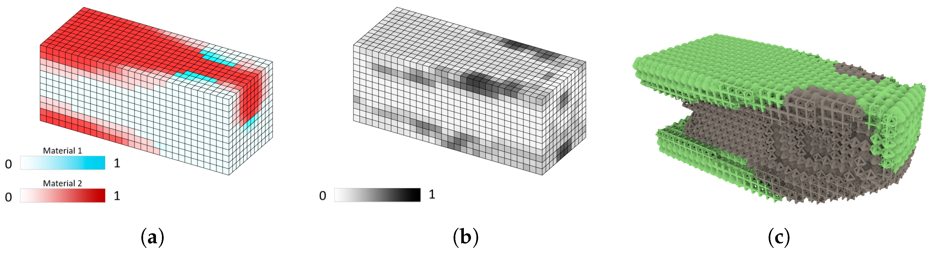
4.1. Multi-Material Multi-Scale TO

For all topology optimization case studies, the value of the force applied was of 60 kN. The overall volume fraction is also common to all cases and it was set at 50% of the total design-domain volume, 25% being allocated to material 1 and the other 25% to material 2. Both design variable intervals were set between [ 0 , 1 ] .
For this work, material 1 was set with a Young’s modulus of E 1 = 145 MPa and material 2 was set with a Young modulus of E 2 = 210 MPa.

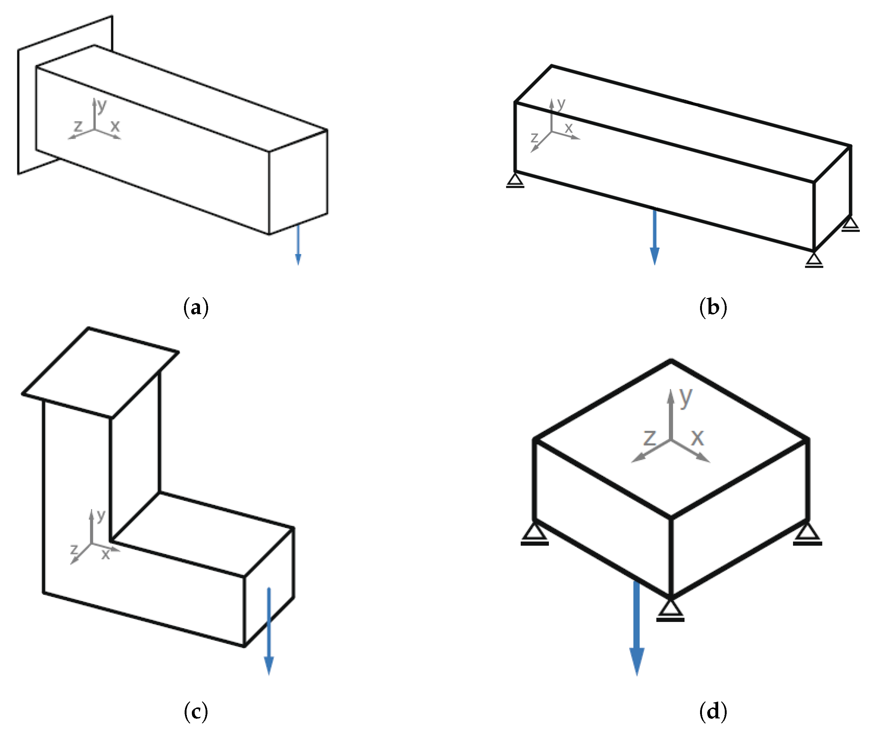
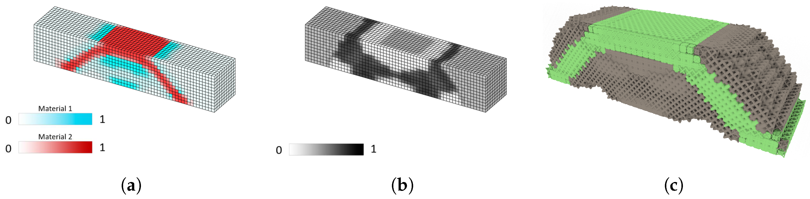
4.1.1. Cantilever Case Study

All the TO results of the six geometries for the Cantilever case study are presented. This structure is fully constrained at one end (to the left of the figure) and free to move at the opposite end (to the right of the figure). It has a 12 × 12 finite element-sized square section with 30 unit cells of length.
The Cantilever case study (Figure 7a) starts as a solid bar with a square section. One end of the bar is fully constrained, with neither linear nor rotational degrees of freedom, whereas the other end is free to translate and rotate. A vertical force, pointing downwards, is applied to the middle of the horizontal bottom edge of the free end of the bar. These properties should translate to a TO result that is symmetric in relation to a plane parallel to x y .
The renders of the following results of this case study are presented in Figure A1, Figure A2, Figure A3, Figure A4, Figure A5 and Figure A6.
Figure 8a, Figure 9a, Figure 10a, Figure 11a, Figure 12a and Figure 13a illustrate the density as well as the material distribution within the volume domain. On the constrained area (to the left of the illustration), there is a significant concentration of material 2 at the top and the bottom faces along the whole width of the structure. The material tends to shape similarly to a nozzle when we move away from the constraint end towards the free end and culminates on the area where the force is applied. Towards the free end of the cantilever structure, material 1 was allocated (less stiff) near the area where the force is applied. The qualitative density as well as the material distribution is identical to all geometries in this case study.

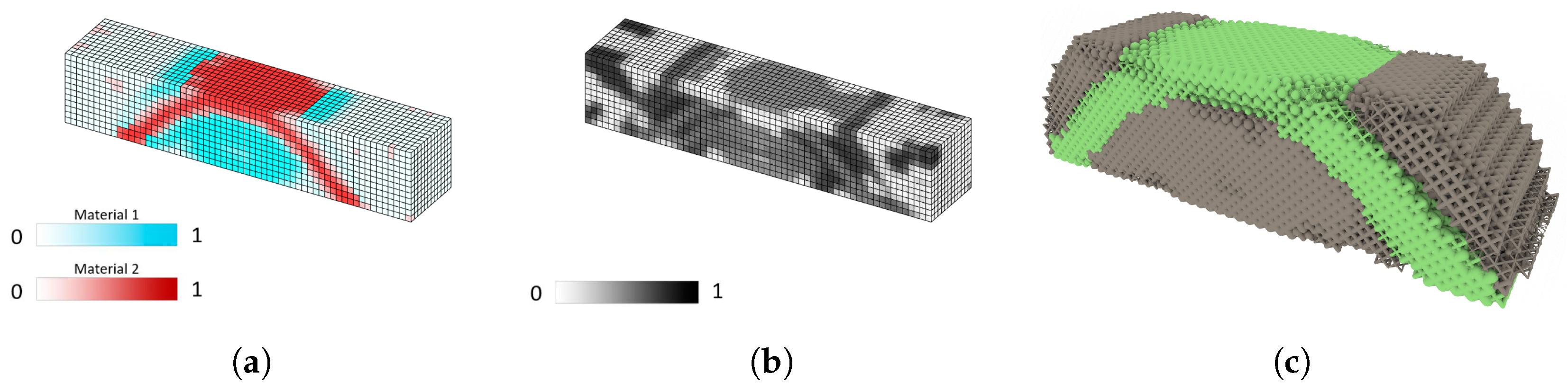
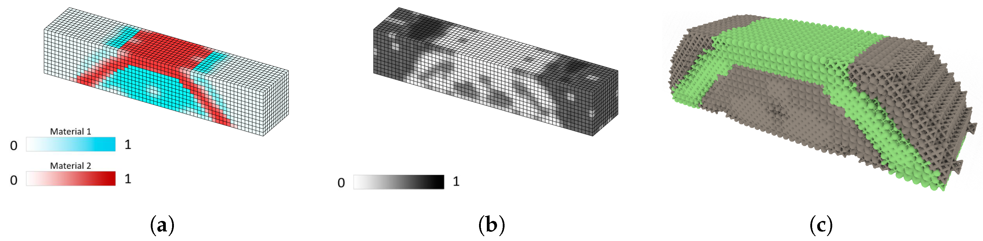
4.1.2. Messerchimitt–Bolkow–Blohm (MBB) Case Study

The renders of the following results of this case study are presented in Figure A7, Figure A8, Figure A9, Figure A10, Figure A11 and Figure A12.
In this case study (Figure 7b), a solid bar with a square section is horizontally supported in the four bottom edges of the solid. On these four points, the structure is fully constrained, meaning there is no linear or rotational movement. A downwards vertical force is applied to the centre of the upper face of the bar. This case study can perhaps be regarded as a bridge, and the TO should result in a final structure that is symmetrical to a plane parallel to x y as well as to y z .
From the figures that illustrate the density distribution within the design domain (Figure 14a, Figure 15a, Figure 16a, Figure 17a, Figure 18a and Figure 19a), we can observe that there is a distribution of material 2 (in red) in the shape of an arc, connecting the constrained elements, on the bottom face, to the middle of the top face of the structure. This arc-shaped density distribution of material 2 (stiffer material) is identical (from a qualitative point of view) in all the MBB case studies of the different geometries.
The material and density distribution of material 1 (in blue) in the structure, on the other hand, presents slight differences in term of “filling” the inner part of the arc previously described with material 2, which is worth highlighting.

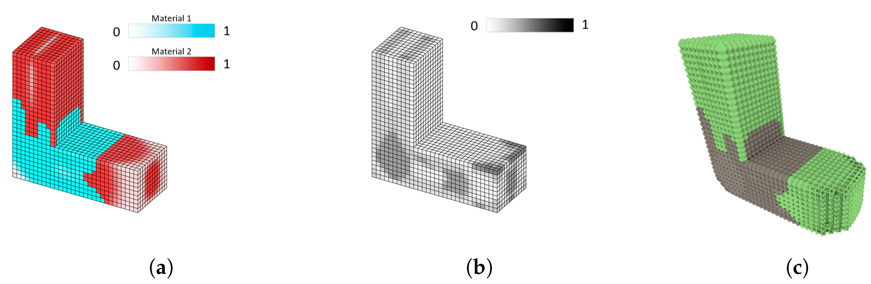
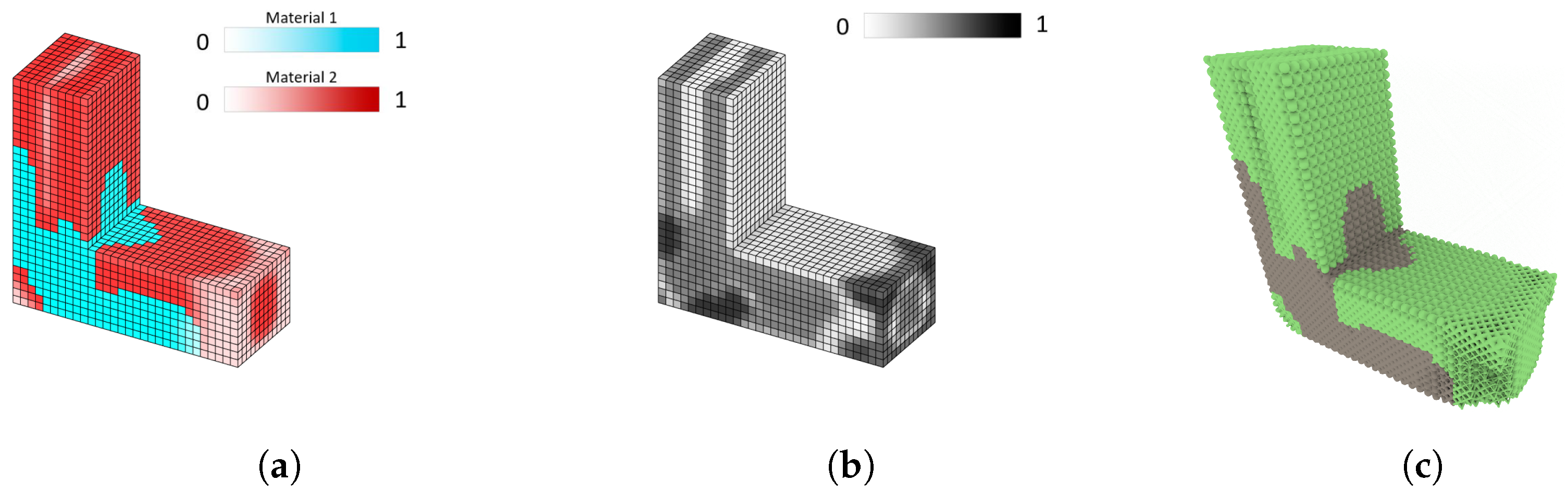
4.1.3. Hook Case Study

The renders of the following results of this case study are presented in Figure A13, Figure A14, Figure A15, Figure A16, Figure A17 and Figure A18.
The Hook case study starts with a structure in the L shape with a square section. The top square section is fully constrained, whereas the other square section (other end of the “L” shaped structure) is free to move. A downward vertical force is to be applied on the centre of the free-to-move section. This case study TO should result in a final structure that is symmetrical in relation to a plane parallel to x y .
The case studies that are presented below are quite similar in terms of overall relative density distribution and present qualitatively identical areas where material 1 and material 2 was allocated. In the figures that relate to relative density distribution (Figure 20a, Figure 21a, Figure 22a, Figure 23a, Figure 24a and Figure 25a), the salient observation that can be made is that there is a concentration of material 1 (in blue, less stiff) on the corner area of the L-shaped structure, which then switches into material 2 (in red, stiffer) as we move from the corner towards the constrained and free edges. The exact positioning of material does not appear to be the same for the different geometries presented, although the qualitative position of it within the structure is, in a way, identical.

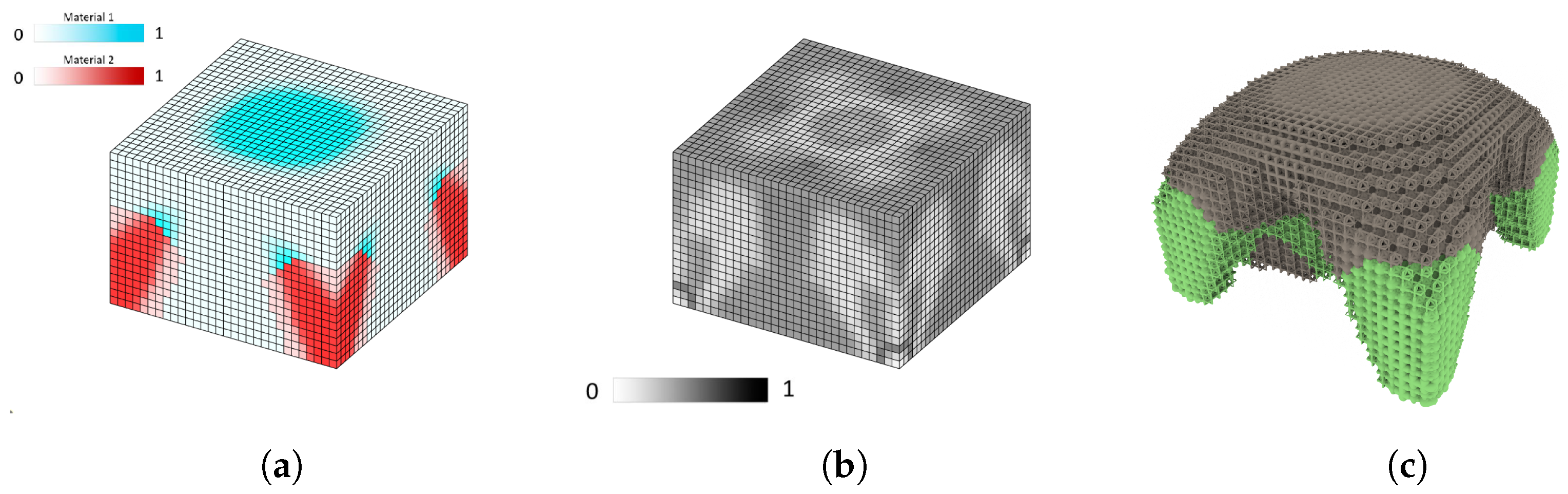
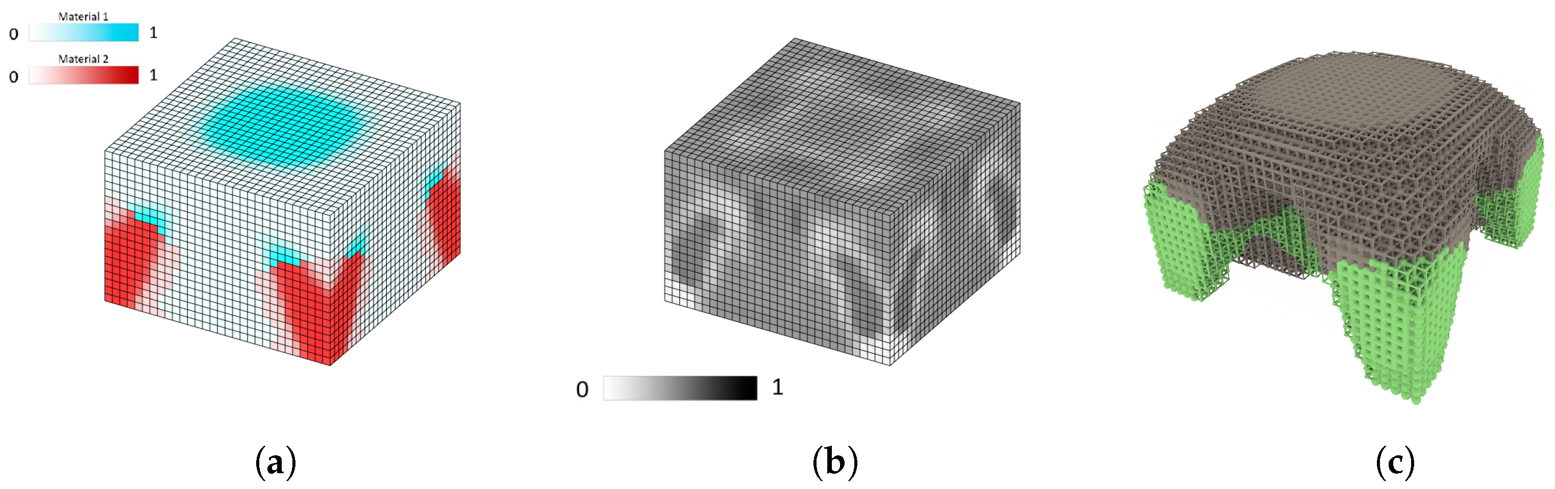
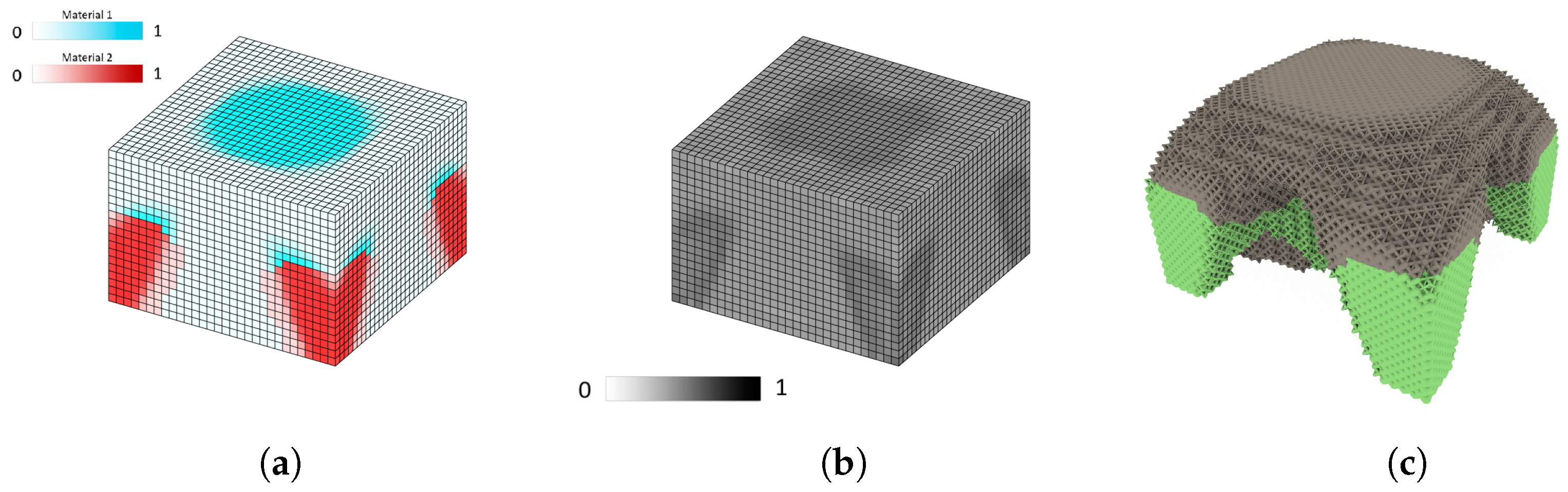
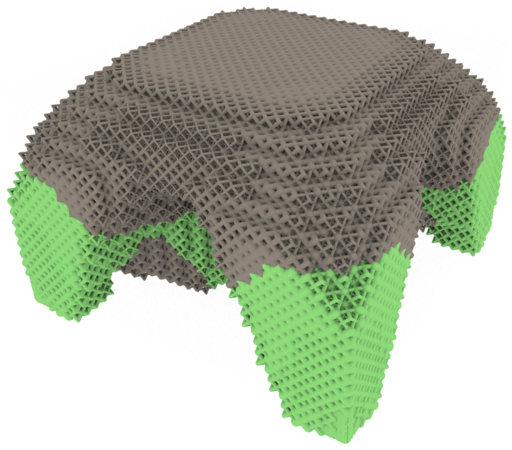
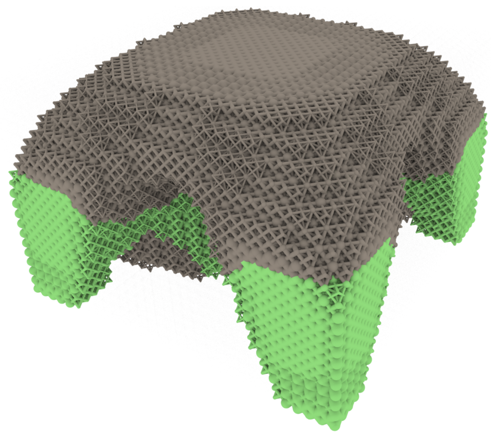
4.1.4. Wheel (“Table Top”) Case Study

The renders of the following results of this case study are presented in Figure 26, Figure 27, Figure 28, Figure 29, Figure 30 and Figure 31.
The Wheel case study features a parallel piped structure that is supported in the four bottom corners. These corners are fully constrained. A downward vertical force is applied to the center of the bottom face of the structure. This case study might resemble a table top. The TO final structure should be symmetrical to a plane parallel to x y and y z .
In the Wheel case studies, the qualitative similarities of density as well as material distribution amongst the various case studies with different geometries can be observed. On the bottom corners of the design domain, all figures show a concentration of material 2 (in red) starting from the support points, where the structure is fully constrained. From this point upwards and inwards, the “legs” of the final structure develop towards the middle of the design domain and eventually change into material 1 (in blue).

4.2. Results Comparison

The compliance values at which the TO has converged is displayed in bar-type graphs. In order to check the efficiency of combining the outer and inner branches of the geometries proposed, the converged compliance values for three different scenarios are presented for each geometry: when only the outer branches are used ( ρ e x t = 1 , in orange), for when only the inner branches are used ( ρ e x t = 0 , in blue), and finally for when the aspect ratio varies freely within the 0 to 1 scope ( ρ e x t [ 0 , 1 ] , in grey), resulting in a combination of the outer and inner branches.
An immediate observation that can be made from the information presented in Figure 32 and Figure 33 is that the use of the full geometry presented, meaning having a combination of the outer and inner branches of the geometry, tends to give a slightly or even a substantially better result (compliance value wise) when compared to the cases where the aspect ratio was set to 0 or 1, either only inner branches or only outer branches.
Figure 32a,b illustrate the compliance results obtained in the Cantilever case study for the six geometries. From the values of the grey bars (representing the 0–1 aspect ratio interval), the geometry with the lowest value of compliance was the Diagonal Cross + Inner Cross geometry. On the other hand, the geometry with the greatest compliance value was the Diagonal Cross + Inner Cage (for the scenario where the aspect ratio varies from 0 to 1 only).
Regarding the results obtained for the MBB case study (Figure 32c,d), the geometry which resulted in the lowest value of compliance was the Diagonal Cross + Inner Cage. On the other hand, the geometry with the highest value of compliance was for both the Cube + Inner Diagonal Cross and the Diagonal Cross + Inner Diagonal Cross geometries. The final compliance results are within 3.5 % from each other (for the 0–1 aspect ratio scenario).
In the figures presented next (Figure 33a,b), it can be verified that from the Cube + Inner Diagonal Cross geometry resulted the lowest value of compliance for the Hook case study. The Diagonal Cross + Inner Diagonal Cross geometry had the highest value of compliance (for the 0–1 aspect ratio scenario). As a side note, both of these geometries share the same inner branches architecture, although they have different outer branches.
Regarding the Wheel case study, given the information from Figure 33c,d the geometry which resulted in the lowest value of compliance was the Cross + Diamond geometry. The geometry with the highest value of compliance was the Diagonal Cross + Inner Cross geometry (for the 0–1 aspect ratio scenario). The final compliance values for the 0–1 aspect ratio scenario of all 6 geometries vary roughly 1 % from one another.

5. Concluding Remarks

The novelties of this work stem from the creation of six surrogate models that effectively represent the elasticity tensor of each of the six geometries concerning two design variables: relative density and aspect ratio. These design variables determine both the volume occupied by the geometry within the designated finite element volume and the distribution of that volume between the inner and outer branches of the geometry.
For the topology optimization process, surrogate models were created for six hierarchical lattice materials during the first solution phase. The creation of these models involved constructing a database based on material homogenization theory. Here, it should be noted that considerable computational time was needed for each run. It was assumed that the number of finite elements would adequately represent the strut-based lattice shape and that the lattice-independent branches would not significantly intersect for the entire density range. While this assumption did not prevent the creation of a surrogate model, it could result in failure to converge for a multi-scale topology optimization. Therefore, it is essential to consider branch interception when using the PILM principle to develop new surrogate models. A set of sampling points for each elasticity tensor were calculated and later interpolated using LSM with a 7th order polynomial, which resulted in the coefficients of the best fitting surface to those points.
Next, multi-scale, multi-variable topology optimization was performed. The overall average improvement considering the compliance result when the [ 0 , 1 ] interval of aspect ratio was considered, and the second best result (either with the result from having aspect ratio set as 0 or 1) was 3.32 % . In more detail, in the Cantilever case study the average improvement in compliance value, in the same circumstances as previously described, was 1.9 % . In the MBB case study, the improvement was 1.67 % . In the Wheel case study, the improvement was 1.7 % . Lastly, the improvement in the Hook case study was 8.02 % . These improvements bring to light the advantages of the combination of the outer and inner branches presented into more complex although better-performing geometries.
Furthermore, the amount of finite elements seems to have been sufficient, given that none of the TO runs resulted in a divergent behaviour. The number of iterations enabled the TO process to run until an acceptable level of convergence had been reached.

Author Contributions

Conceptualization, J.S., A.S. (Abdolrasoul Sohouli) and A.S. (Afzal Suleman); methodology, J.S., A.S. (Abdolrasoul Sohouli) and A.S. (Afzal Suleman); software, J.S. and A.S. (Abdolrasoul Sohouli); validation, J.S.; formal analysis, J.S., A.S. (Abdolrasoul Sohouli); investigation, J.S., A.S. (Abdolrasoul Sohouli) and A.S. (Afzal Suleman); data curation, J.S. and A.S. (Abdolrasoul Sohouli); writing—original draft preparation, J.S.; writing—review and editing, A.S. (Abdolrasoul Sohouli) and A.S. (Afzal Suleman); visualization, J.S.; supervision, A.S. (Abdolrasoul Sohouli) and A.S. (Afzal Suleman); project administration, A.S. (Afzal Suleman). All authors have read and agreed to the published version of the manuscript.

Funding

The authors acknowledge Fundação para a Ciência e a Tecnologia (FCT) for its financial support via the project LAETA Base Funding (DOI: 10.54499/UIDB/50022/2020).

Data Availability Statement

The data presented in this study is available upon request.

Acknowledgments

Afzal Suleman acknowledges the NSERC Canada Research Chair and Discovery funding programs.

Conflicts of Interest

The authors declare no conflicts of interest.

Appendix A

Figure A1. Render: Cross + Diamond geometry applied to the Cantilever case study.
Jcs 08 00124 g0a1
Figure A2. Render: Cube + Inner diagonal cross geometry applied to the Cantilever case study.
Jcs 08 00124 g0a2
Figure A3. Render: Diagonal cross + Diamond geometry applied to the Cantilever case study.
Jcs 08 00124 g0a3
Figure A4. Render: Diagonal cross + Inner cage geometry applied to the Cantilever case study.
Jcs 08 00124 g0a4
Figure A5. Render: Diagonal cross + Inner cross geometry applied to the Cantilever case study.
Jcs 08 00124 g0a5
Figure A6. Render: Diagonal cross + Inner diagonal cross geometry applied to the Cantilever case study.
Jcs 08 00124 g0a6
Figure A7. Render: Cross + Diamond geometry applied to the MBB case study.
Jcs 08 00124 g0a7
Figure A8. Render: Cube + Inner diagonal cross geometry applied to the MBB case study.
Jcs 08 00124 g0a8
Figure A9. Render: Diagonal cross + Diamond geometry applied to the MBB case study.
Jcs 08 00124 g0a9
Figure A10. Render: Diagonal cross + Inner cage geometry applied to the MBB case study.
Jcs 08 00124 g0a10
Figure A11. Render: Diagonal cross + Inner cross geometry applied to the MBB case study.
Jcs 08 00124 g0a11
Figure A12. Render: Diagonal cross + Inner diagonal cross geometry applied to the MBB case study.
Jcs 08 00124 g0a12
Figure A13. Render: Cross + Diamond geometry applied to the Hook case study.
Jcs 08 00124 g0a13
Figure A14. Render: Cube + Inner diagonal cross geometry applied to the Hook case study.
Jcs 08 00124 g0a14
Figure A15. Render: Diagonal cross + Diamond geometry applied to the Hook case study.
Jcs 08 00124 g0a15
Figure A16. Render: Diagonal cross + Inner cage geometry applied to the Hook case study.
Jcs 08 00124 g0a16
Figure A17. Render: Diagonal cross + Inner cross geometry applied to the Hook case study.
Jcs 08 00124 g0a17
Figure A18. Render: Diagonal cross + Inner diagonal cross geometry applied to the Hook case study.
Jcs 08 00124 g0a18
Figure A19. Render: Cross + Diamond geometry applied to the Wheel case study.
Jcs 08 00124 g0a19
Figure A20. Render: Cube + Inner diagonal cross geometry applied to the Wheel case study.
Jcs 08 00124 g0a20
Figure A21. Render: Diagonal cross + Diamond geometry applied to the Wheel case study.
Jcs 08 00124 g0a21
Figure A22. Render: Diagonal cross + Inner cage geometry applied to the Wheel case study.
Jcs 08 00124 g0a22
Figure A23. Render: Diagonal cross + Inner cross geometry applied to the Wheel case study.
Jcs 08 00124 g0a23
Figure A24. Render: Diagonal cross + Inner diagonal cross geometry applied to the Wheel case study.
Jcs 08 00124 g0a24

References

  1. Chuang, W.; Jihong, Z.; Manqiao, W.; Jie, H.; Han, Z.; Lu, M.; Chenyang, L.; Zhang, W. Multi-scale design and optimization for solid-lattice hybrid structures and their application to aerospace vehicle components. Chin. J. Aeronaut. 2021, 34, 386–398. [Google Scholar]
  2. Jankovics, D.; Barari, A. Customization of automotive structural components using additive manufacturing and topology optimization. IFAC-PapersOnLine 2019, 52, 212–217. [Google Scholar] [CrossRef]
  3. Bendsøe, M.P.; Kikuchi, N. Generating optimal topologies in structural design using a homogenization method. Comput. Methods Appl. Mech. Eng. 1988, 71, 197–224. [Google Scholar] [CrossRef]
  4. Wang, C.; Gu, X.; Zhu, J.; Zhou, H.; Li, S.; Zhang, W. Concurrent design of hierarchical structures with three-dimensional parameterized lattice microstructures for additive manufacturing. Struct. Multidiscip. Optim. 2020, 61, 869–894. [Google Scholar] [CrossRef]
  5. Deshpande, V.S.; Fleck, N.A.; Ashby, M.F. Effective properties of the octet-truss lattice material. J. Mech. Phys. Solids 2001, 49, 1747–1769. [Google Scholar] [CrossRef]
  6. Queheillalt, D.T.; Wadley, H.N. Cellular metal lattices with hollow trusses. Acta Mater. 2005, 53, 303–313. [Google Scholar] [CrossRef]
  7. Clough, E.C.; Ensberg, J.; Eckel, Z.C.; Ro, C.J.; Schaedler, T.A. Mechanical performance of hollow tetrahedral truss cores. Int. J. Solids Struct. 2016, 91, 115–126. [Google Scholar] [CrossRef]
  8. Wu, J.; Sigmund, O.; Groen, J.P. Topology optimization of multi-scale structures: A review. Struct. Multidiscip. Optim. 2021, 63, 1455–1480. [Google Scholar] [CrossRef]
  9. Wang, Y.; Hu, D.; Wang, H.; Zhang, T.; Yan, H. Practical design optimization of cellular structures for additive manufacturing. Eng. Optim. 2020, 52, 1887–1902. [Google Scholar] [CrossRef]
  10. Watts, S.; Arrighi, W.; Kudo, J.; Tortorelli, D.A.; White, D.A. Simple, accurate surrogate models of the elastic response of three-dimensional open truss micro-architectures with applications to multiscale topology design. Struct. Multidiscip. Optim. 2019, 60, 1887–1920. [Google Scholar] [CrossRef]
  11. Ypsilantis, K.I.; Kazakis, G.; Lagaros, N.D. An efficient 3D homogenization-based topology optimization methodology. Comput. Mech. 2021, 67, 481–496. [Google Scholar] [CrossRef]
  12. Nguyen, C.H.P.; Choi, Y. Concurrent density distribution and build orientation optimization of additively manufactured functionally graded lattice structures. Comput.-Aided Des. 2020, 127, 102884. [Google Scholar] [CrossRef]
  13. Imediegwu, C.; Murphy, R.; Hewson, R.; Santer, M. Multiscale structural optimization towards three-dimensional printable structures. Struct. Multidiscip. Optim. 2019, 60, 513–525. [Google Scholar] [CrossRef]
  14. Murphy, R.; Imediegwu, C.; Hewson, R.; Santer, M. Multiscale structural optimization with concurrent coupling between scales. Struct. Multidiscip. Optim. 2021, 63, 1721–1741. [Google Scholar] [CrossRef]
  15. Costa, M.; Sohouli, A.; Suleman, A. Multi-scale and multi-material topology optimization of gradient lattice structures using surrogate models. Compos. Struct. 2022, 289, 115402. [Google Scholar] [CrossRef]
  16. Andreassen, E.; Clausen, A.; Schevenels, M.; Lazarov, B.S.; Sigmund, O. Efficient topology optimization in MATLAB using 88 lines of code. Struct. Multidiscip. Optim. 2011, 43, 1–16. [Google Scholar] [CrossRef]
  17. Gao, J.; Luo, Z.; Xia, L.; Gao, L. Concurrent topology optimization of multiscale composite structures in Matlab. Struct. Multidiscip. Optim. 2019, 60, 2621–2651. [Google Scholar] [CrossRef]
  18. Sigmund, O. Morphology-based black and white filters for topology optimization. Struct. Multidiscip. Optim. 2007, 33, 401–424. [Google Scholar] [CrossRef]
  19. Eckrich, M.; Arrabiyeh, P.A.; Dlugaj, A.M.; May, D. Structural topology optimization and path planning for composites manufactured by fiber placement technologies. Compos. Struct. 2022, 289, 115488. [Google Scholar] [CrossRef]
  20. Guedes, J.; Kikuchi, N. Preprocessing and postprocessing for materials based on the homogenization method with adaptive finite element methods. Comput. Methods Appl. Mech. Eng. 1990, 83, 143–198. [Google Scholar] [CrossRef]
  21. Xia, L.; Breitkopf, P. Design of materials using topology optimization and energy-based homogenization approach in Matlab. Struct. Multidiscip. Optim. 2015, 52, 1229–1241. [Google Scholar] [CrossRef]
  22. Michel, J.C.; Moulinec, H.; Suquet, P. Effective properties of composite materials with periodic microstructure: A computational approach. Comput. Methods Appl. Mech. Eng. 1999, 172, 109–143. [Google Scholar] [CrossRef]
  23. Ashby, M.F. The properties of foams and lattices. Philos. Trans. R. Soc. A Math. Phys. Eng. Sci. 2006, 364, 15–30. [Google Scholar] [CrossRef] [PubMed]
  24. Leary, M.; Mazur, M.; Williams, H.; Yang, E.; Alghamdi, A.; Lozanovski, B.; Zhang, X.; Shidid, D.; Farahbod-Sternahl, L.; Witt, G.; et al. Inconel 625 lattice structures manufactured by selective laser melting (SLM): Mechanical properties, deformation and failure modes. Mater. Des. 2018, 157, 179–199. [Google Scholar] [CrossRef]
  25. Dong, G.; Tang, Y.; Zhao, Y.F. A 149 line homogenization code for three-dimensional cellular materials written in matlab. J. Eng. Mater. Technol. 2019, 141, 011005. [Google Scholar] [CrossRef]
  26. Zhang, X.; Leary, M.; Tang, H.; Song, T.; Qian, M. Selective electron beam manufactured Ti-6Al-4V lattice structures for orthopedic implant applications: Current status and outstanding challenges. Curr. Opin. Solid State Mater. Sci. 2018, 22, 75–99. [Google Scholar] [CrossRef]
  27. Xiao, Z.; Yang, Y.; Xiao, R.; Bai, Y.; Song, C.; Wang, D. Evaluation of topology-optimized lattice structures manufactured via selective laser melting. Mater. Des. 2018, 143, 27–37. [Google Scholar] [CrossRef]
  28. Xu, S.; Shen, J.; Zhou, S.; Huang, X.; Xie, Y.M. Design of lattice structures with controlled anisotropy. Mater. Des. 2016, 93, 443–447. [Google Scholar] [CrossRef]
  29. Venugopal, V.; Hertlein, N.; Anand, S. Multi-material topology optimization using variable density lattice structures for additive manufacturing. Procedia Manuf. 2021, 53, 327–337. [Google Scholar] [CrossRef]
  30. Liu, K.; Tovar, A. An efficient 3D topology optimization code written in Matlab. Struct. Multidiscip. Optim. 2014, 50, 1175–1196. [Google Scholar] [CrossRef]
Figure 1. Cross + Diamond geometry. (a) ρ e x t = 0 . (b) ρ e x t = 0.5 . (c) ρ e x t = 1 .
Jcs 08 00124 g001
Figure 2. Cube + Inner Diagonal Cross geometry. (a) ρ e x t = 0 . (b) ρ e x t = 0.5 . (c) ρ e x t = 1 .
Jcs 08 00124 g002
Figure 3. Diagonal Cross + Diamond geometry. (a) ρ e x t = 0 . (b) ρ e x t = 0.5 . (c) ρ e x t = 1 .
Jcs 08 00124 g003
Figure 4. Diagonal Cross + Inner Cage geometry. (a) ρ e x t = 0 . (b) ρ e x t = 0.5 . (c) ρ e x t = 1 .
Jcs 08 00124 g004
Figure 5. Diagonal Cross + Inner cross geometry. (a) ρ e x t = 0 . (b) ρ e x t = 0.5 . (c) ρ e x t = 1 .
Jcs 08 00124 g005
Figure 6. Diagonal Cross + Inner Diagonal Cross geometry. (a) ρ e x t = 0 . (b) ρ e x t = 0.5 . (c) ρ e x t = 1 .
Jcs 08 00124 g006
Figure 7. Case studies [30]. (a) Cantilever case study. (b) Messerchimitt–Bolkow–Blohm (MBB) case study. (c) Hook case study. (d) Wheel case study.
Jcs 08 00124 g007
Figure 8. Cantilever case study: Cross + Diamond geometry. (a) Relative density distribution—material 1 in blue, material 2 in red. (b) Aspect ratio distribution. (c) Render: Cross + Diamond geometry applied to the Cantilever case study.
Jcs 08 00124 g008
Figure 9. Cantilever case study: Cube + Inner diagonal cross geometry. (a) Relative density distribution—material 1 in blue, material 2 in red. (b) Aspect ratio distribution. (c) Render: Cube + Inner diagonal cross geometry applied to the Cantilever case study.
Jcs 08 00124 g009
Figure 10. Cantilever case study: Diagonal cross + Diamond geometry. (a) Relative density distribution—material 1 in blue, material 2 in red. (b) Aspect ratio distribution. (c) Render: Diagonal cross + Diamond geometry applied to the Cantilever case study.
Jcs 08 00124 g010
Figure 11. Cantilever case study: Diagonal cross + Inner cage geometry. (a) Relative density distribution—material 1 in blue, material 2 in red. (b) Aspect ratio distribution. (c) Render: Diagonal cross + Inner cage geometry applied to the Cantilever case study.
Jcs 08 00124 g011
Figure 12. Cantilever case study: Diagonal cross + Inner cross geometry. (a) Relative density distribution—material 1 in blue, material 2 in red. (b) Aspect ratio distribution. (c) Render: Diagonal cross + Inner cross geometry applied to the Cantilever case study.
Jcs 08 00124 g012
Figure 13. Cantilever case study: Diagonal cross + Inner diagonal cross geometry. (a) Relative density distribution—material 1 in blue, material 2 in red. (b) Aspect ratio distribution. (c) Render: Diagonal cross + Inner diagonal cross geometry applied to the Cantilever case study.
Jcs 08 00124 g013
Figure 14. MBB case study: Cross + Diamond geometry. (a) Relative density distribution—material 1 in blue, material 2 in red. (b) Aspect ratio distribution. (c) Render: Cross + Diamond geometry applied to the MBB case study.
Jcs 08 00124 g014
Figure 15. MBB case study: Cube + Inner diagonal cross geometry. (a) Relative density distribution—material 1 in blue, material 2 in red. (b) Aspect ratio distribution. (c) Render: Cube + Inner diagonal cross geometry applied to the MBB case study.
Jcs 08 00124 g015
Figure 16. MBB case study: Diagonal cross + Diamond geometry. (a) Relative density distribution—material 1 in blue, material 2 in red. (b) Aspect ratio distribution. (c) Render: Diagonal cross + Diamond geometry applied to the MBB case study.
Jcs 08 00124 g016
Figure 17. MBB case study: Diagonal cross + Inner cage geometry. (a) Relative density distribution—material 1 in blue, material 2 in red. (b) Aspect ratio distribution. (c) Render: Diagonal cross + Inner cage geometry applied to the MBB case study.
Jcs 08 00124 g017
Figure 18. MBB case study: Diagonal cross + Inner cross geometry. (a) Relative density distribution—material 1 in blue, material 2 in red. (b) Aspect ratio distribution. (c) Render: Diagonal cross + Inner cross geometry applied to the MBB case study.
Jcs 08 00124 g018
Figure 19. MBB case study: Diagonal cross + Inner diagonal cross geometry. (a) Relative density distribution—material 1 in blue, material 2 in red. (b) Aspect ratio distribution. (c) Render: Diagonal cross + Inner diagonal cross geometry applied to the MBB case study.
Jcs 08 00124 g019
Figure 20. Hook case study: Cross + Diamond geometry. (a) Relative density distribution—material 1 in blue, material 2 in red. (b) Aspect ratio distribution. (c) Render: Cross + Diamond geometry applied to the Hook case study.
Jcs 08 00124 g020
Figure 21. Hook case study: Cube + Inner diagonal cross geometry. (a) Relative density distribution—material 1 in blue, material 2 in red. (b) Aspect ratio distribution. (c) Render: Cube + Inner diagonal cross geometry applied to the Hook case study.
Jcs 08 00124 g021
Figure 22. Hook case study: Diagonal cross + Diamond geometry. (a) Relative density distribution—material 1 in blue, material 2 in red. (b) Aspect ratio distribution. (c) Render: Diagonal cross + Diamond geometry applied to the Hook case study.
Jcs 08 00124 g022
Figure 23. Hook case study: Diagonal cross + Inner cage geometry. (a) Relative density distribution—material 1 in blue, material 2 in red. (b) Aspect ratio distribution. (c) Render: Diagonal cross + Inner cage geometry applied to the Hook case study.
Jcs 08 00124 g023
Figure 24. Hook case study: Diagonal cross + Inner cross geometry. (a) Relative density distribution—material 1 in blue, material 2 in red. (b) Aspect ratio distribution. (c) Render: Diagonal cross + Inner cross geometry applied to the Hook case study.
Jcs 08 00124 g024
Figure 25. Hook case study: Diagonal cross + Inner diagonal cross geometry. (a) Relative density distribution—material 1 in blue, material 2 in red. (b) Aspect ratio distribution. (c) Render: Diagonal cross + Inner diagonal cross geometry applied to the Hook case study.
Jcs 08 00124 g025
Figure 26. Wheel case study: Cross + Diamond geometry. (a) Relative density distribution—material 1 in blue, material 2 in red. (b) Aspect ratio distribution. (c) Render: Cross + Diamond geometry applied to the Wheel case study.
Jcs 08 00124 g026
Figure 27. Wheel case study: Cube + Inner diagonal cross geometry. (a) Relative density distribution—material 1 in blue, material 2 in red. (b) Aspect ratio distribution. (c) Render: Cube + Inner diagonal cross geometry applied to the Wheel case study.
Jcs 08 00124 g027
Figure 28. Wheel case study: Diagonal cross + Diamond geometry. (a) Relative density distribution—material 1 in blue, material 2 in red. (b) Aspect ratio distribution. (c) Render: Diagonal cross + Diamond geometry applied to the Wheel case study.
Jcs 08 00124 g028
Figure 29. Wheel case study: Diagonal cross + Inner cage geometry. (a) Relative density distribution—material 1 in blue, material 2 in red. (b) Aspect ratio distribution. (c) Render: Diagonal cross + Inner cage geometry applied to the Wheel case study.
Jcs 08 00124 g029
Figure 30. Wheel case study: Diagonal cross + Inner cross geometry. (a) Relative density distribution—material 1 in blue, material 2 in red. (b) Aspect ratio distribution. (c) Render: Diagonal cross + Inner cross geometry applied to the Wheel case study.
Jcs 08 00124 g030
Figure 31. Wheel case study: Diagonal cross + Inner diagonal cross geometry. (a) Relative density distribution—material 1 in blue, material 2 in red. (b) Aspect ratio distribution. (c) Render: Diagonal cross + Inner diagonal cross geometry applied to the Wheel case study.
Jcs 08 00124 g031
Figure 32. Compliance comparison between geometries. (a) Compliance comparison between TO final results for 3 geometries, each geometry with ρ e x t = 0 or ρ e x t = 1 or ρ e x t varying from 0 to 1. (b) Compliance comparison between TO final results for 3 geometries, each with ρ e x t = 0 or ρ e x t = 1 or ρ e x t varying from 0 to 1. (c) Compliance comparison between TO final results for 3 geometries, each with ρ e x t = 0 or ρ e x t = 1 or ρ e x t varying from 0 to 1. (d) Compliance comparison between TO final results for 3 geometries, each with ρ e x t = 0 or ρ e x t = 1 or ρ e x t varying from 0 to 1.
Jcs 08 00124 g032
Figure 33. Compliance comparison between geometries. (a) Compliance comparison between TO final results for 3 geometries, each with ρ e x t = 0 or ρ e x t = 1 or ρ e x t varying from 0 to 1. (b) Compliance comparison between TO final results for 3 geometries, each with ρ e x t = 0 or ρ e x t = 1 or ρ e x t varying from 0 to 1. (c) Compliance comparison between TO final results for 3 geometries, each with ρ e x t = 0 or ρ e x t = 1 or ρ e x t varying from 0 to 1. (d) Compliance comparison between TO final results for 3 geometries, each with ρ e x t = 0 or ρ e x t = 1 or ρ e x t varying from 0 to 1.
Jcs 08 00124 g033
Disclaimer/Publisher’s Note: The statements, opinions and data contained in all publications are solely those of the individual author(s) and contributor(s) and not of MDPI and/or the editor(s). MDPI and/or the editor(s) disclaim responsibility for any injury to people or property resulting from any ideas, methods, instructions or products referred to in the content.

