Solving Some Graph Problems in Composite 3D Printing Using Spreadsheet Modeling

Abstract

The use of composite materials in additive manufacturing has significant potential and prospects for development. However, the 3D printing of composite materials also has some challenges, such as tool path planning and optimization, material distribution and planning, optimization of printing parameters, and others. Graph theory may be suitable for solving some of them. Many practical problems can be modeled as problems of identifying subsets of graph vertices or edges with certain extremal properties. Such problems belong to the category of graph extremal problems. Some of these problems can be represented as integer linear programming problems, for which, in order to solve, modifications of simplex method can be used. These methods are supported by MS Excel Solver add-in, which suggests the possibility of solving these problems effectively with its help. The task of implementing procedures for solving such problems by means of standard engineering software seems to be possible. This paper aims to develop efficient spreadsheet models of some extremal problems for graphs of higher strength in order to prove the feasibility and to unify the procedures of solving such problems via the MS Excel Solver add-in. Several spreadsheet models based on the graph representation by its expanded incidence matrix, while specifying a vector of unknowns as the vector of binary variables associated with vertices or edges of the sought parts of the graph, have been developed and proven to be efficient for solving such problems by simplex method via the MS Excel Solver add-in.

1. Introduction

Today, the use of polymer materials in 3D printing technology (additive manufacturing) has significant potential for development. Three-dimensional (3D) printing is a process of creating three-dimensional objects by adding layers of material on top of each other and using composite materials leads to enhanced mechanical, thermal, or electrical properties [1]. Additive manufacturing with composite materials offers several advantages over traditional single-material printing. Composite materials offer the ability to engineer specific material properties by selecting appropriate combinations of matrix materials and reinforcements [2]. This allows for tailoring strength, stiffness, other mechanical properties, conductivity, electrical conductivity, chemical resistance, and more to meet the application requirements. In addition, 3D printing allows for the use of various types of matrix materials and reinforcements, such as thermoplastics, thermosets, carbon fibers, glass fibers, metal particles, and more. This allows for complex geometries and intricate designs, optimizing designs, and reducing weight while maintaining mechanical integrity. However, it is worth noting that the 3D printing of composite materials also poses some challenges [3]. Some of them, for instance toolpath planning and optimization, material allocation and scheduling, optimizing printing parameters, can be solved using graph theory. Similar problems occur in the development of interconnection topology in 3D MID technology (Three-Dimensional Molded Interconnect Devices) of injection-molded thermoplastic circuit carriers with in-built conductive traces and pads which can be regarded as a kind of 3D PCB [4].

Graph algorithms, such as shortest path algorithms, can be used to plan and optimize the toolpath for 3D printing [5,6]. The toolpath is the sequence of movements that the 3D printer’s nozzle or laser follows to create the object. By modeling the printing environment as a graph, with nodes representing printable locations and edges representing feasible movements, algorithms can find efficient toolpaths that minimize travel time, reduce the number of retractions or tool head movements, and optimize the overall printing process. Graph theory can assist in optimizing material allocation and scheduling in multi-material or multi-object printing scenarios [7]. By representing the objects or materials as nodes and their dependencies or constraints as edges, graph algorithms can find optimal allocation strategies, minimize material changes or swaps, and schedule the printing process to minimize downtime and maximize efficiency.

These problems mostly refer to the category of NP problems, whose solution algorithms are mainly based on forms of variant search. Computer support of this process is implemented by specialized, expensive application software packages. The methodological basis for solving such problems is created by graph theory. Graph theory is a mathematical field that deals with the study of graphs, which are mathematical structures used to model relationships between objects. Graph theory has applications in many different fields, including computer science, research of operations in complex systems, physics, biology, social sciences, and many others.

Computer graph algorithms are used in many applications such as routing and scheduling problems, recommendation systems, social networks, and data mining [8]. In physics, graphs are used to model the behavior of physical systems such as molecules, crystals, and networks [9,10]. Graph theory is used in biology to model and analyze biological networks such as gene regulatory networks, protein interaction networks, food webs, in the study of epidemiology, and the spread of infectious diseases [11]. In social sciences, graphs are used to study social networks and social structures and determine the level of influence of subjects in these networks [12]. Graph theory is also actively used in operations research of complex systems to model and solve problems such as network optimization, transportation planning, and facility location [13,14,15]. Graph algorithms can then be used to find the optimal allocation of resources that maximize effectiveness of the system. It is necessary, though, to separate the optimization problems [16,17]. Graph theory is used to model such networks and to find optimal paths or routes that minimize cost, time, or other factors. By using graph theory algorithms and techniques, it is possible to find optimal solutions to a wide range of telecommunication or computer network design and optimization problems [18,19,20].

The most common extremal problems on graphs of wide practical application are the problems of finding minimum vertex and edge covers, minimum dominant and maximum independent sets of vertices and edges, maximum clique, critical path, minimal spanning tree, and minimum Hamiltonian cycle of a graph. Such problems belong to the category of graph extremal problems. Some of these problems can be represented as integer linear programming problems, the solving of which can be achieved with modifications of the simplex method.

The simplex method is a widely used algorithm for solving linear programming problems that is used to find the optimality solution to a system of linear equations, subject to constraints in the form of linear inequalities [21]. The simplex method works by starting at a feasible solution and iteratively improving the solution until the optimal one is reached. This method is used in a wide range of applications, including production planning, resource allocation, financial modeling, and transportation planning. The algorithm has been extended and modified over time to handle more complex problems, such as mixed-integer programming and nonlinear programming [22].

Variants of modeling and solving some of these problems by MS Excel Solver are proposed in [23,24]. The mathematical formulation of extremal problems as Boolean linear programming problems in [23,25,26] are given individually for every graph configuration, which does not allow unifying the procedures of creating and solving a spreadsheet model. Moreover, some models include redundant constraints, e.g., a constraint on the number of edges/vertices in minimal edge/vertex covers, which makes sense if the edge cover is supposed to be the graph spanning tree. The authors of [23,27] propose modeling the problems on finding the smallest set covering and packing, the smallest dominant set of vertices, the shortest path on a graph, and the minimum Hamiltonian cycle as integer linear programming problems when using analytical representation of a graph by its adjacency matrix. Thus, a matrix of unknowns with the dimension of the graph adjacency matrix is used to find the required subset of vertices, thereby limiting the use of the method to graphs with the number of vertices N ≤ (N₀)^1/2, where N₀ is the Solver limit for the number of integer variables, which in non-professional versions does not exceed 100, so the vertex set power for the studied graph is limited to 10. In [28], the graph is represented by reduced adjacency matrix with dimension (N−1), which makes it possible to slightly extend the modeled graph range and to propose modeling and solution of minimal path and minimal spanning tree problems. In [24], a Solver-oriented spreadsheet model of the graph, the critical path problem is based on specifying the graph structure by an extended incidence matrix (i.e., matrix containing also a basic node) with using the matrix of unknowns of the same dimension as the extended incidence matrix, thus limiting the method application to graphs with N × M ≤ N₀, where N and M are the powers of the graph vertex and edge sets, respectively. N₀ is the Solver limit for integer variables.

Thus, the task of implementing procedures for solving such problems by means of standard engineering software seems to be actual. This paper aims to develop efficient spreadsheet models of some extremal problems for graphs of higher strength in order to prove the feasibility and unify the procedures of solving such problems via the MS Excel Solver add-in.

The basic novelty of the work consists in finding the way to represent a number of combinatorial problems on graphs as binary linear programming problems in Microsoft Excel. The very idea of solving some of the considered problems on graphs not by using algorithms common for each type of problem but as binary linear programming problems belongs to S. P. Ighlin [19]. However, the presenting the proposed BLP models as spreadsheet models appears to be too cumbersome, which makes it difficult to use the Microsoft Excel Solver add-in for solving these problems. At the same time, the version of spreadsheet models developed by the authors is the most compact one and does not require additional built-in functions for matrix transformation, thus making it affordable for common users. An additional result of this research is also the extension of the types of problems that can be solved directly by MS Excel Solver by the simplex method, including extreme graph problems, previously considered beyond the scope of MS Excel (please see the Supplementary Materials).

The area of application of the proposed models extends far beyond 3D printing. The urgency of such solutions became even more acute in Ukraine during the armed hostilities, when many small- and medium-sized enterprises were forced to relocate their business. The usual logistics chains were destroyed, and the identification and optimization of new ones had to be carried out as quickly as possible without the involvement of additional funds or personnel, using the most common software, primarily the Microsoft Office package. The developed problem models allow these tasks to be solved with very few staff skills. It should also be noted that many of the optimal target hitting problems also come down to the tasks discussed above. These problems are to be solved in combat situations by mid-level military personnel using, among others, smartphones, which precludes the use of special software.

2. Methods

2.1. Extremal Graph Problems under Study: Definition and Relationship

Minimum vertex and edge cover problems. A vertex and an edge of a graph G(V,U) cover each other if they are incident to each other. Therefore, edge u_ij ⊂ {v_i, v_j} covers vertices v_i and v_j, and each of these vertices covers edge u_ij [25,29].

Definition 1.

A subset of vertices V* ⊂ V is called a vertex cover of graph G(U,V) if each edge u_ij of U is incident to at least one vertex of V. A cover of graph G is called minimum vertex cover (MVC) if the number of vertices in it is the smallest one among all the covers of graph G. The number of vertices in the smallest cover of graph G is called vertex cover number of graph G and is denoted β(G).

Definition 2.

An edge cover of a graph G(V,U) is such a subset of its edges U* ⊆ U that all vertices of V are incident to at least one edge of this subset U*. The edge cover is called minimum line cover (MLC) or minimum edge cover (MEC) if it contains the smallest possible number of edges to cover all vertices [26,30]. The problems of finding minimum vertex and edge cover in a graph are called the minimum vertex and edge cover problems, respectively, and are NP-complete [25]. The problems are modeled as optimization problems on graphs; for each of these problems, specific solution algorithms were developed, providing for particular software implementation [31,32,33]: Maximum inner independent vertex set, maximum independent edge set, and the maximum clique problems. The concept of graph cover is closely related to the notion of internal independent vertex set [34].

Definition 3.

A set of vertices V′ ⊂ V is called independent (or internally stable) if no vertices of this set are adjacent to each other. That is, for any ∀v_i ∈ V′, ∀v_j ∈ V′, no edge u_ij ⊂ {v_i, v_j} exists. An independent set of the largest size is called the maximum one. The cardinality of the maximum independent set of graph G is called the independence number (internal stability number, non-density) and denoted by α(G).

The problem of finding the largest independent set in a graph is called the maximum independent set problem and is NP-complete as well [35]. The relation between vertex cover and vertex independent set of graphs is given by the following theorem: set Z of vertices of graph G = (V, U) is the minimum cover of this graph if and only if Y = V\Z is the maximum independent set. Thus, maximum independent vertex sets correspond to the complements of minimum vertex covers and the independence number α(G), and vertex cover number β(G) of a graph G are related by: α(G) + β(G)= |V|, where |V| is the vertex number [32]. It means that all vertices of the graph, which do not belong to the minimum cover, will form the maximum independent set, and vice versa, all vertices of the graph not belonging to the maximum independent set form its minimum cover. Thus, the problems about minimum cover and maximum independent set are dual; the solution of one of them automatically gives the solution of the other one as well.

Definition 4.

A subset of vertices V” ⊂ V of graph G = (V, U) is called a clique if any two vertices of V” are adjacent, i.e., the stemmed subgraph G”(V”,U”) is a complete (strongly connected) graph. A clique of largest strength is called a maximum one. The number of vertices in the graph maximum clique is called density, or clique number, and is denoted by φ(G). The complement graph of graph G is a graph G** with the same set of vertices as G, any two vertices connected by an edge, only when they are not connected by an edge in graph G. Therefore, a subset of graph G vertices forms a clique only when it is independent in the complement graph G**. Hence φ(G) = α(G**). Therefore, to get the maximum clique of graph G, we just have to construct the complement graph G** and find the maximum independent set in it [36]. Thus, it can be stated that the solution of each of the three above-described problems can be reduced to the solution of any one of them.

Definition 5.

The set of edges of graph G = (V, U) is called an independent edge set or a matching on G if no two edges in it have a common vertex. The size of matching of maximum strength is called the matching number of G and is denoted by ν(G). The maximum matching problem for a given graph is a problem of finding the matching set of the largest strength [37]. Considering the above dependencies between different extreme sets of vertices, at first, we set out to solve one of these problems—the minimum cover problem, the solving of which would give the maximum independent set and the maximum clique as well.

2.2. Extremal Graph Problems under Study: Spreadsheet Modeling

Suppose it is required to find the minimum vertex cover (MVC) of graph G(V,U) (Figure 1). Graph G can be specified by the matrix A = {a_ik}, in which each row corresponds to a vertex of the graph, and each column—to an edge of the graph [38,39]. This matrix differs from the canonical incidence matrix by having rows representing all nodes, including the base node. Hereafter, we refer to this matrix as the extended incidence matrix A. Introducing a row representing the base node is redundant in terms of the analytical representation of the graph, but greatly simplifies the formation of a spreadsheet model in the media similar to Microsoft Excel. Matrix A element a_ik takes value 1 if vertex v_i covers edge u_k, (v_i ∈ u_k), and 0 otherwise. Then, finding minimum vertex cover in a graph G is equivalent to finding its part G*(V*), V* ⊂ V, whose matrix A* has the least number of rows covering all columns of this matrix by values of 1. Then, the model of this problem takes the form:

$$\begin{array}{cccc}\forall i,\forall k,& k=\overline{1,T},& i=\overline{1,N}& \begin{array}{c}{\displaystyle {\displaystyle \sum }_{i=1}^N}{x}_{ik}\ge 1\end{array}\end{array}$$

(1)

$$\begin{array}{cccc}\forall i,\forall k,& k=\overline{1,T},& i=\overline{1,N}& \begin{array}{c}\begin{array}{c}{x}_{ik}=0\vee 1\end{array}\end{array}\end{array}$$

(2)

$$\begin{array}{ccc}\forall \mathrm{i},\forall \mathrm{k},& \mathrm{k}=\overline{1,\mathrm{T}},& \mathrm{i}=\overline{1,\mathrm{N}}\end{array}\begin{array}{c} \begin{array}{c}{\mathrm{x}}_{\mathrm{ik}}\le {\mathrm{a}}_{\mathrm{ik}}\end{array}\end{array}$$

(3)

$$\mathrm{F}={\displaystyle \sum }_{\mathrm{i}=1}^{\mathrm{N}}\left({\mathrm{n}}_{\mathrm{i}}|{\displaystyle \sum }_{\mathrm{k}=1}^{\mathrm{T}}{\mathrm{x}}_{\mathrm{ik}}\ge 1\right)|\to \min$$

(4)

where x_ik is a value of the element of the unknowns matrix A* at the intersection of the i-th row (corresponding to i-th vertex) and k-th column (corresponding to k-th edge); T is cardinality of the edge set U of the graph G; N is cardinality of the vertex set V of the graph G; n_i is a row corresponding to i-th vertex covering at least one graph edge (${\displaystyle \sum }_{\mathrm{K}=1}^{\mathrm{T}}{\mathrm{x}}_{\mathrm{ik}}>0$); F—number of vertices of the required subgraph with degree not less than 1, i.e., the number of rows in the matrix of unknowns for which ${\displaystyle \sum }_{\mathrm{K}=1}^{\mathrm{T}}{\mathrm{x}}_{\mathrm{ik}}\ge 1$.

The target function F can be calculated in Microsoft Excel using the built-in COUNTIF function, which returns the number of matrix rows meeting a certain condition. The problem thus presented is reduced to a Boolean optimization problem with a discontinuous objective function. Solving such problems is supported by Solver add-in Microsoft Excel version 10 and higher, using evolutionary programming methods based on genetic algorithms. Thus, to form a spreadsheet model of the problem in Microsoft Excel and to solve it, it is necessary to form an extended incidence matrix of the original graph and a matrix of unknowns of the same size and to input formulas reflecting (1–4) into the corresponding cells of the Excel sheet. These are formulas for the sum (SUM) for each column of the matrix of unknowns, to form the constraint (1) and for each row of the matrix of unknowns to form the target function (4) argument and the final formula for the target function COUNTIF with the parameters for the condition of sum across rows exceeding 0.5 (i.e., non-zero values considering the precision of setting an integer value). Then, the problem model is to be transferred into Solver by setting additional constraints of Booleanity of matrix of unknowns (binarity constraint for cells of matrix of unknowns) and belonging of the graph G* to the graph G, i.e., (x_ik ≤ a_ik). As a solving method, the evolutionary method should be chosen.

The evolutionary programming method is based on genetic algorithms and due to the specificity of these algorithms, it can return different solutions even with the same initial conditions. Therefore, it is recommended to repeat the search procedure several times, increasing the convergence and changing the starting points. Each of the search procedures returns the vertex cover and gradually approaches (over 3–4 procedures) its minimum value.

3. Results

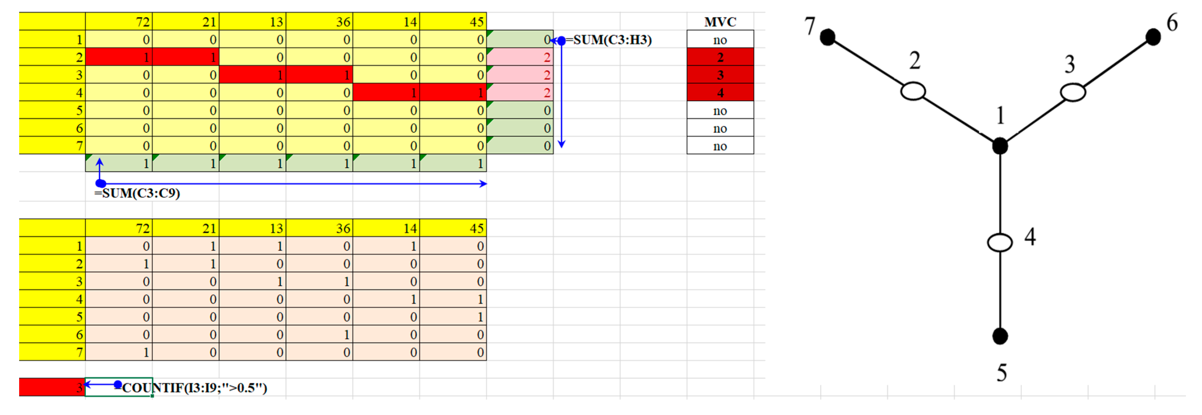
3.1. Minimum Vertex Cover Problem

For the initial testing of the proposed method, graph G presented in [32,40,41] was chosen. Graph G and its spreadsheet model based on its extended incidence matrix are shown in Figure 1 and

Table 1. MS Excel spreadsheet model of the MVC problem for graph G (Figure 1).

Cells	Formulas or Initial Values	Model Component
C3:H9	0	Matrix of unknowns. After performing the search procedure, filled rows of the matrix identify the vertices of MVC of graph G
C14:H20	0∧1	The incidence matrix of the original graph G
I3	SUM(C3:H3), extended to I4:I9	Number of edges covered by a vertex included in the cover G* of graph G
C10	SUM(C3:C9), extended to D10:H10	Number of MVC vertices covering each edge of graph G
C22	COUNTIF(I3:I9; “>0.5”)	Objective function: vertex cover number of graph G β(G) (number of vertices in MVC), which is equal to the number of non-zero cells in the range I3:I9

and

Table 2. MS Excel spreadsheet model of the constraints of the MVC problem for graph G (Figure 1).

Constraint	Constraint Content
C3:H9=binary	The Boolean character of variables in the matrix of unknowns
$C$3:$H$9<=$C$14:$H$20	Condition of belonging the MVC vertices to graph G (V* ⊂ V)
$C$10:$H$10>=1	The requirement of covering every edge of the graph G by at least one of the vertices v ∈ V*

.

After transferring the problem model to the Solver dialog box and setting the convergence parameter to 0.00001, we run the solution search procedure for minimizing the objective function by evolutionary method for 10 times. For nine runs, we obtained values of the objective function of 3, with MVC = {2, 3, 4}, which corresponds to the result obtained in [40,41]. Once the search procedure returned a target cell value of 4 with MVC = {1, 2, 3, 4}. After reducing the convergence to 0.0000001, the value of the objective function of 3 and MVC = {2, 3, 4} was obtained. A similar result was obtained after changing the initial search values. In all cases, a search time limit of 30 s was set, with actual search times ranging from 4 to 15 s.

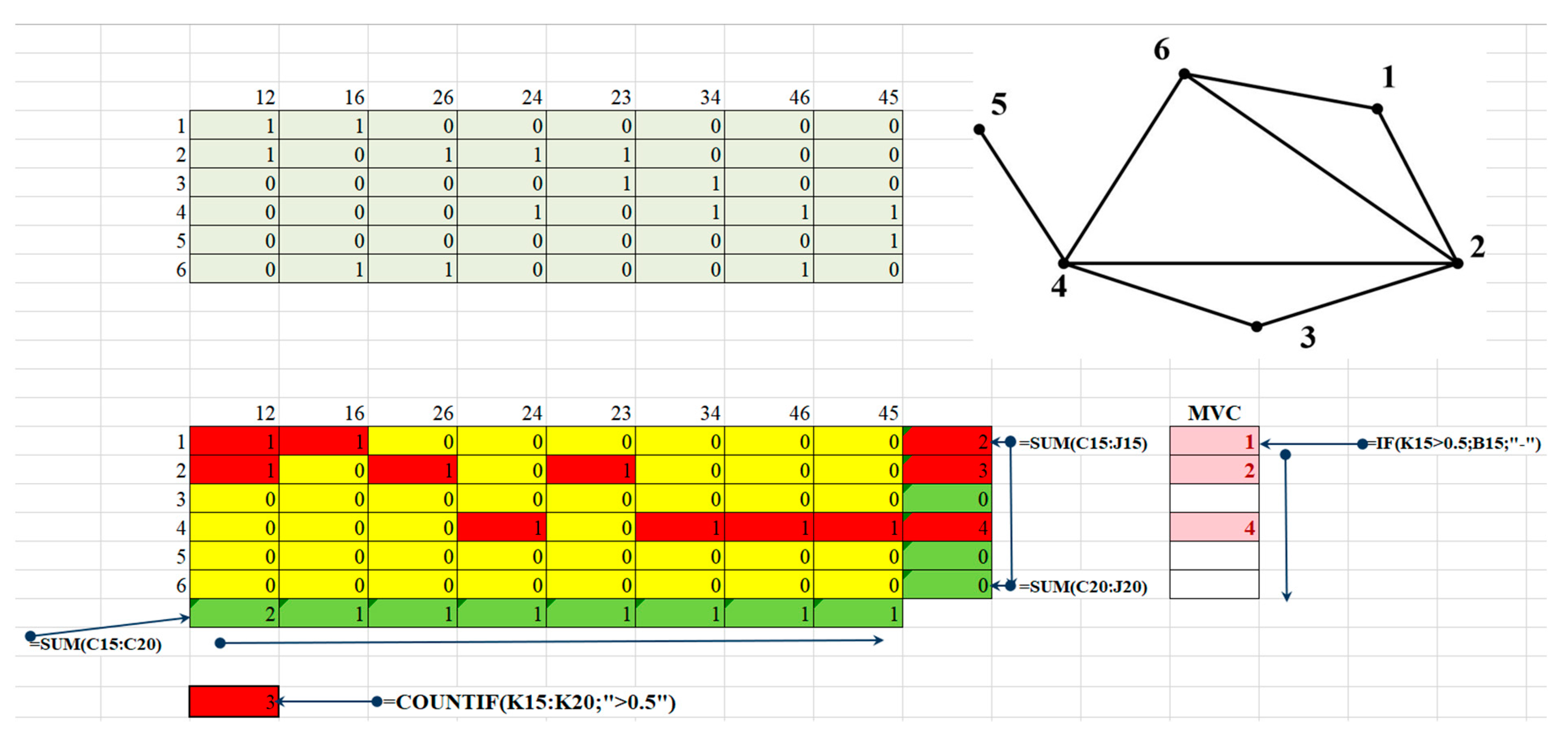
For smaller graphs [42,43], as one would expect, the search took less time. For the graph in Figure 2, a similar problem model was built and similar constraints were set. The result of solving the problem (Figure 2) was obtained 10 consecutive times with the search time never exceeding 5 s.

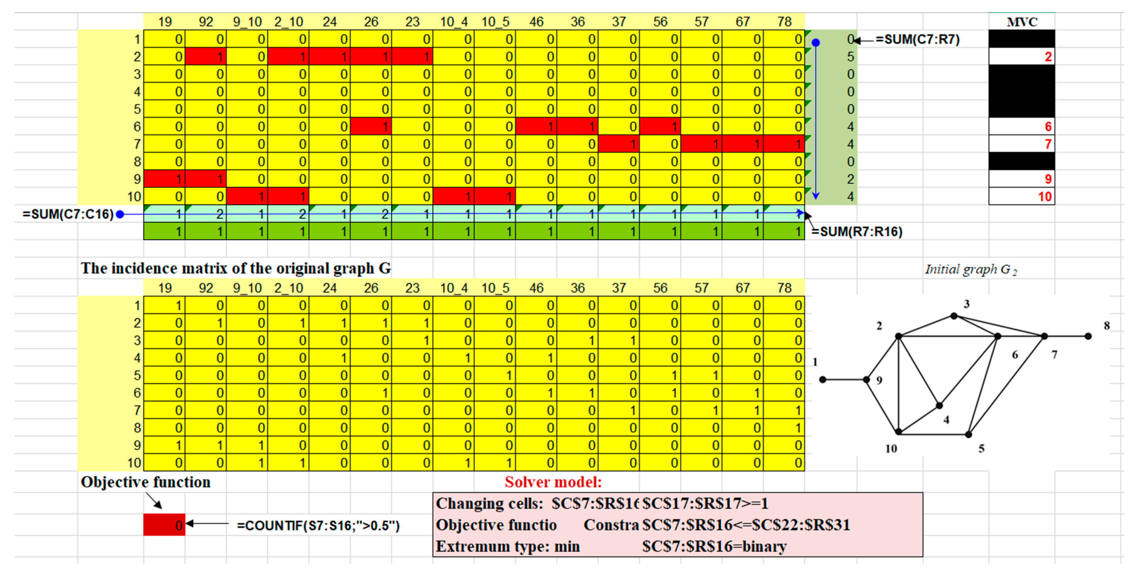
To test the suitability of the method for graphs of higher strength, the method was tested on several graphs, one of which is shown in the figure below (Figure 3) together with a spreadsheet model of the MVC problem for this graph G₂ on an Excel sheet and Solver model parameters.

Having set the convergence parameter to 0.00001, we implemented the procedure for minimizing the target function by evolutionary search 8 times, gradually increasing the convergence to 0.0000000001, with a change of the starting point in some cases (tests 2, 7, and 8). A search time limit of 30 s was set. The search did not last more than 25 s. The results of the computational experiment are given in

Table 3. Results of identifying the graph G₂ MVC and the corresponding cover number by evolutionary search in MS Excel Solver.

Test	Cover Number β(G) and MVC Composition (Vertices Involved in the MVC)
	1	2	3	4	5	6	7	8
1	6 (2, 3, 6, 7, 9, 10)	6 (2, 6, 7, 8, 9, 10)	6 (2, 6, 7, 8, 9, 10)	5 (2, 6, 7, 9, 10)	5 (2, 6, 7, 9, 10)	5	5	5
2	7 (3, 4, 6, 7, 8, 9, 10)	6 (2, 6, 7, 8, 9, 10)	6 (2, 6, 7, 8, 9, 10)	(2, 6, 7, 8, 9, 10)	5 (2, 6, 7, 9, 10)	5	5	5
3	7 (3, 4, 6, 7, 8, 9, 10)	6 (2, 6, 7, 8, 9, 10)	6 (2, 6, 7, 8, 9, 10)	5 (2, 6, 7, 9, 10)	5 (2, 6, 7, 9, 10)	5	5	5
4	6 (2, 3, 6, 7, 9, 10)	5 (2, 6, 7, 9, 10)	5 (2, 6, 7, 9, 10)	5 (2, 6, 7, 9, 10)	5 (2, 6, 7, 9, 10)	5	5	5
5	5 (2, 6, 7, 9, 10)	5 (2, 6, 7, 9, 10)	5 (2, 6, 7, 9, 10)	5 (2, 6, 7, 9, 10)	5 (2, 6, 7, 9, 10)	5	5	5
6	6 (2, 3, 6, 7, 9, 10)	6 (2, 3, 6, 7, 9, 10)	5 (2, 6, 7, 9, 10)	5 (2, 6, 7, 9, 10)	5 (2, 6, 7, 9, 10)	5	5	5
7	6 (2, 3, 6, 7, 9, 10)	6 (2, 3, 6, 7, 9, 10)	5 (2, 6, 7, 9, 10)	5 (2, 6, 7, 9, 10)	5 (2, 6, 7, 9, 10)	5	5	5
8	6 (2, 6, 7, 8, 9, 10)	6 (2, 6, 7, 8, 9, 10)	6 (2, 3, 6, 7, 9, 10)	6 (2, 6, 7, 8, 9, 10)	5 (2, 6, 7, 9, 10)	5	5	5
9	6 (2, 6, 7, 8, 9, 10)	5 (2, 6, 7, 9, 10)	5 (2, 6, 7, 9, 10)	5 (2, 6, 7, 9, 10)	5 (2, 6, 7, 9, 10)	5	5	5
10	6 (2, 6, 7, 8, 9, 10)	5 (2, 6, 7, 9, 10)	5 (2, 6, 7, 9, 10)	5 (2, 6, 7, 9, 10)	5 (2, 6, 7, 9, 10)	5	5	5

.

As Table 3 shows, for all cases the graph MVC consisting of vertices {2, 6, 7, 9, 10} was obtained over several search procedures. It corresponds to the maximum inner independent vertex set {1, 3, 4, 5, 8}, being the difference of the set of graph vertices V and the MVC V*.

As computational experiments show, while the number of vertices and edges of a graph increases, it becomes more and more difficult to obtain a globally optimal solution to the MVC problem and the associated problem of determining the maximum independent set by the evolutionary search. The evolutionary search method was applied because of the discontinuous nature of the target function COUNTIF. In order to change the search method, an attempt was made to change the model of the problem, so that the COUNTIF function could be replaced by the SUM function. To do this, the items of the target function are to take only one of two values 0∨1, where 1 corresponds to the vertex included in MVC (i.e., there are values other than 0 in the row corresponding to the vertex) and 0 otherwise. This can be achieved by introducing into the problem model a vector of unknowns $\mathrm{X}=\left\{{\mathrm{x}}_{\mathrm{i}}\right\},\begin{array}{cc}\mathrm{i}=\overline{1,\mathrm{N},}& {\mathrm{x}}_{\mathrm{i}}=0\vee 1\end{array}$, whose N components will be associated with the vertices of the graph, and take value 1 if the vertex is included in the MVC, and 0 in the opposite case [30].

Then, using, as before, the extended incidence matrix A = {a_ik} to define the structure of the initial graph, the constraint for covering all edges of the graph by the required set of vertices forming MVC can be represented as:

$${\displaystyle \sum }_{\mathrm{i}=1}^{\mathrm{N}}{\mathrm{a}}_{\mathrm{ik}}{\mathrm{x}}_{\mathrm{i}}\ge 1$$

(5)

for each edge, i.e., for each matrix A column, and the model of the problem under consideration assumes the following form:

$$\begin{array}{c}\mathrm{X}=\left\{{\mathrm{x}}_{\mathrm{i}}\right\}, \mathrm{i}=\overline{1,\mathrm{N},} {\mathrm{x}}_{\mathrm{i}}=0\vee 1\\ \forall \mathrm{k},\mathrm{k}=\overline{1,\mathrm{T}} {\displaystyle {\displaystyle \sum }_{\mathrm{i}=1}^{\mathrm{N}}}{\mathrm{a}}_{\mathrm{ik}}{\mathrm{x}}_{\mathrm{i}}\ge 1\\ \mathrm{F}=\mathsf{\beta }\left(\mathrm{G}\right)={\displaystyle {\displaystyle \sum }_{\mathrm{i}=1}^{\mathrm{N}}}{\mathrm{x}}_{\mathrm{i}}\to \min \end{array}$$

(6)

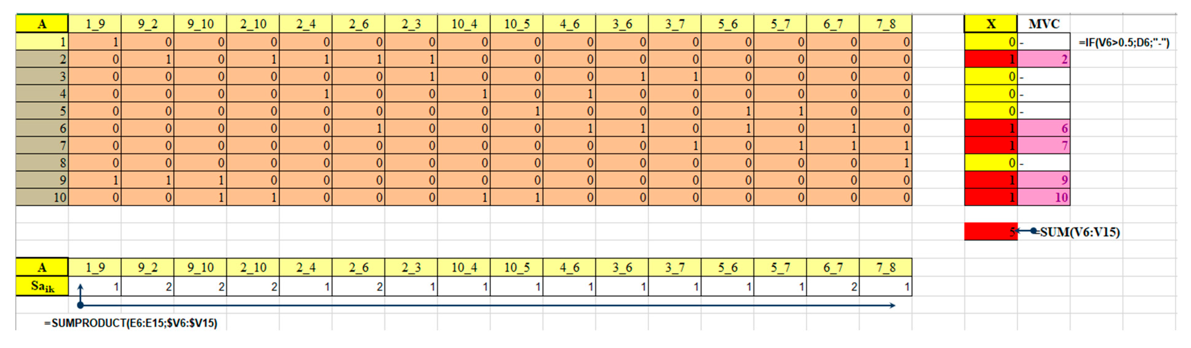
This is a model of a Boolean linear programming (BLP) problem [19]. The simplest way to implement the constraint (5) is to use the built-in Excel function SUMPRODUCT (array1, array2, … [array_n]), which returns the sum of element-by-element products of arrays of the same size. In this case, the spreadsheet model for finding the minimum vertex cover of the graph G₂ (Figure 3) will look as presented in Figure 4 and

Table 4. MS Excel spreadsheet model of the MVC problem for graph G2 (Figure 3) as a Boolean linear programming problem based on the model (6).

Cells	Formulas or Initial Values	Model Component
V6:V15	0	Vector of unknowns X = {xi}. After performing the solution search procedure xi take values 0 ∨ 1
E6:T15	0∧1	The incidence matrix of the original graph G2
E20	=SUMPRODUCT(E6:E15;$V6:$V15), extended to F20:T20	Number of vertices covering each edge of the graph, ${{\displaystyle \sum }}_{\mathrm{i}=1}^{\mathrm{N}}{\mathrm{a}}_{\mathrm{ik}}{\mathrm{x}}_{\mathrm{i}}$
V17	SUM(V6:V15)	Objective function: vertex cover number β(G) of graph G2 (number of vertices in MVC) $\mathrm{F}={\displaystyle \sum }_{\mathrm{i}=1}^{\mathrm{N}}{\mathrm{x}}_{\mathrm{i}}\to \min$, which equals the number of cells with value 1 in the range V6:V15, i.e., ones (xi = 1) in vector X

and

Table 5. MS Excel spreadsheet model of the MVC problem constraints for graph G2 (Figure 3) based on the model (6).

Constraint	Constraint Content
V6:V15=binary	The Boolean character of variables in the matrix of unknowns X, ${\mathrm{x}}_{\mathrm{i}}=0\vee 1$
$E$20:$T$20>=1	The requirement to cover every edge of graph G2 by at least one of the vertices v ∈ V*.

.

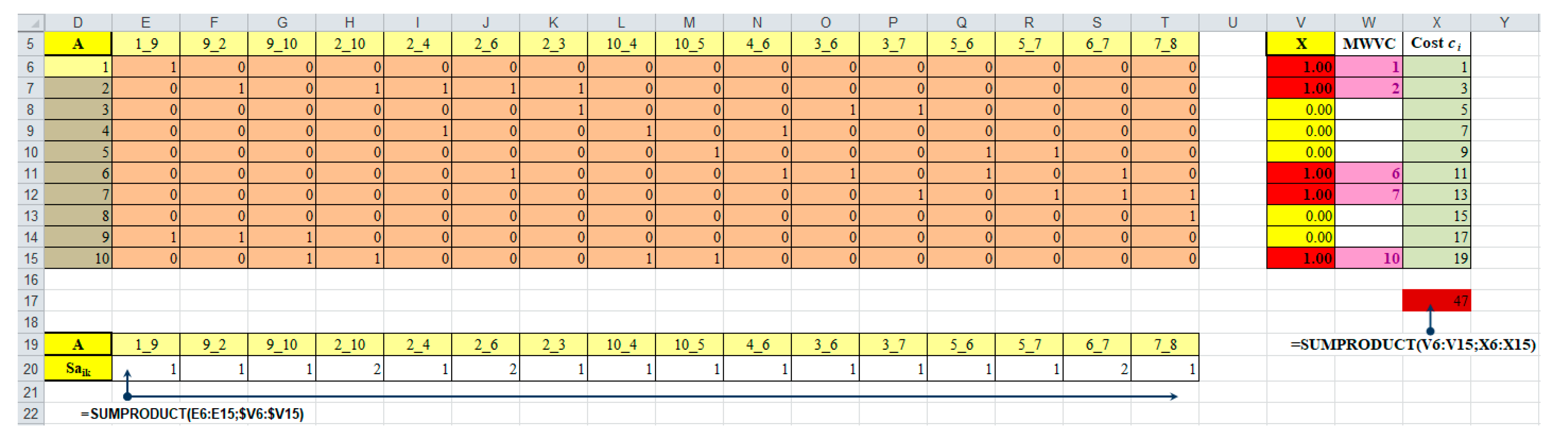
As can be seen from Table 4, all model functions are linear. Transferring the model to the Solver dialog box and setting the optimization criterion to minimization, we chose the simplex search method, taking into account linearity of the model. The solution {2, 6, 7, 9, 10} is obtained almost instantly (Figure 4). This is one of the minimum vertex covers. Using additional constraints on the inclusion of a certain vertex in a cover, we obtain all variants of MVCs. In particular, if the vertex 9 (P27 = 1) is mandatory to be included in the cover, we obtain the solution {2, 6, 7, 9, 10}, i.e., the graph has 2 minimum vertex covers with number of cover of 5.

As seen from the comparison of Table 2, Table 3, Table 4 and Table 5, this variant of problem representation provides a significantly more efficient spreadsheet model suitable for solving by the simplex method which guarantees obtaining globally optimal (minimum) value of coverage number in any case, i.e., the minimum vertex cover. The number of variables in comparison to the previous variant decreases by a factor T, which makes it possible to apply the method for graphs of bigger strength up to 200, since for linear programming problems, the number of Boolean variables in standard versions of Excel Solver cannot exceed 200. A gain in model efficiency compared to [24,30] is achieved by eliminating the formation of the transposed incidence matrix and matrix multiplication operation by taking advantage of the SUMPRODUCT function.

3.2. Minimum Weighted Vertex Cover Problem

The problem differs from the previous one by proposing to minimize not the number of covers, but its value under the assumption that each i-th vertex has a certain cost (weight) c_i. The model of this problem will differ from the previous one only in the objective function $\mathrm{F}={\displaystyle \sum }_{\mathrm{i}=1}^{\mathrm{N}}{\mathrm{c}}_{\mathrm{i}}{\mathrm{x}}_{\mathrm{i}}$, which necessitates the introducing into the spreadsheet model a one-dimensional array containing the costs (weights) of the vertices c_i, $\mathrm{i}=\overline{1,\mathrm{N}}$. After placing this array in cells X6:X15, the objective function formula in cell X17 changes to SUMPRODUCT(V6:V15; X6:X15). Other elements of the problem model remain corresponding Table 4 and Table 5. By transferring the problem model to the Solver parameter window, we obtain the solution shown in Figure 5.

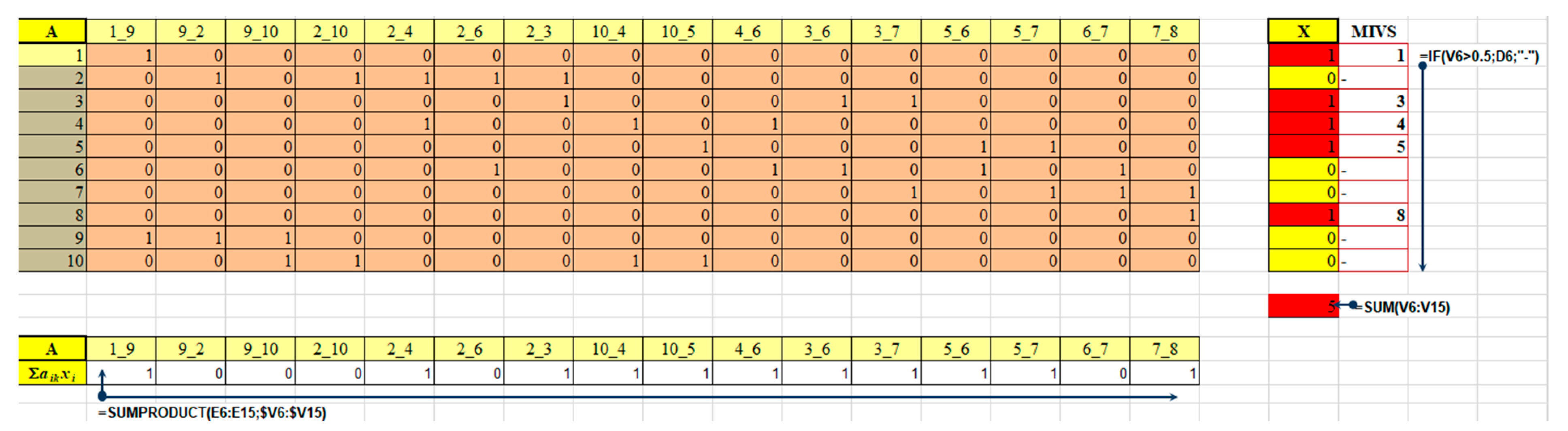
3.3. Maximum Inner Independent Vertex Set (MIVS) Problem

As mentioned before, due to the interrelation between the MIVS and MVC the solution of the MIVC problem can be obtained from the solution of that for MVC as MIVS = G\MVC. However, if the application problem assumes finding exactly the MIVS, a spreadsheet model of the problem can be easily obtained in the same way as the model of the MVC problem. Applying the same notations as in the previous case, and using, as before, the extended graph incidence matrix A = {a_ik} to specify the structure of the original graph, a mathematical model of the MIVS problem can be obtained as (7):

$$\begin{array}{c}\mathrm{X}=\left\{{\mathrm{x}}_{\mathrm{i}}\right\}, \mathrm{i}=\overline{1,\mathrm{N},} {\mathrm{x}}_{\mathrm{i}}=0\vee 1\\ \forall \mathrm{k}, \mathrm{k}=\overline{1,\mathrm{T}} {\displaystyle {\displaystyle \sum }_{\mathrm{i}=1}^{\mathrm{N}}}{\mathrm{a}}_{\mathrm{ik}}{\mathrm{x}}_{\mathrm{i}}\le 1\\ {\displaystyle {\displaystyle \sum }_{\mathrm{i}=1}^{\mathrm{N}}}{\mathrm{x}}_{\mathrm{i}}\to \max \end{array}$$

(7)

It is evident that the spreadsheet model of the problem (7) differs from that presented in Table 4 only in the meaning of the unknowns {x_i}, which are associated with MIVS vertices instead of those included in MVC, and in the meaning and type of the objective function extremum, which will specify the independence number α(G) and will aim at a maximum ${\displaystyle \sum }_{\mathrm{i}=1}^{\mathrm{N}}{\mathrm{x}}_{\mathrm{i}}=\mathsf{\alpha }\left(\mathrm{G}\right)\to \max$ (). The spreadsheet model of the constraints takes the form shown in

Table 6. MS Excel spreadsheet model of the MIVS problem constraints for graph G2 (Figure 3) based on the model (7).

Constraint	Constraint Content
V6:V15=binary	The Boolean character of variables in the matrix of unknowns X, ${\mathrm{x}}_{\mathrm{i}}=0\vee 1$
$E$20:$T$20<=1	The requirement of non-adjacency of vertices belonging to the MIVC of G2

.

All the model functions are linear (Table 4 and Table 6). After transferring the model to the Solver dialog box and setting the optimization criterion to maximum, the simplex search method is run (Figure 6).

The solution {1, 3, 4, 5, 8} is obtained almost immediately. This is one of the maximum independent sets of vertices. By applying additional constraints on the inclusion of certain vertices in an independent set, other variants of the MIVS can be obtained, in particular {3, 4, 5, 8, 9}.

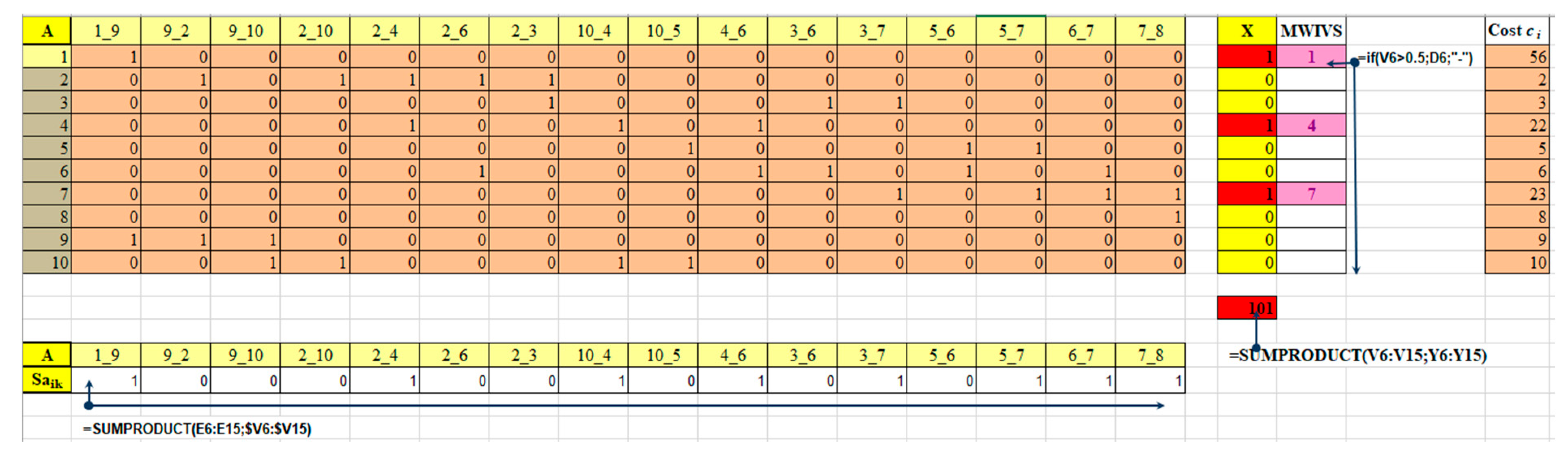
3.4. Minimum Weighted Inner Independent Vertex Set

The problem aims to minimize not the independence number α(G), but its value C under the assumption that each i-th vertex has a certain cost (weight) c_i. The model of this problem differs from the MIVS problem only in the objective function $\mathrm{F}={\displaystyle \sum }_{\mathrm{i}=1}^{\mathrm{N}}{\mathrm{c}}_{\mathrm{i}}{\mathrm{x}}_{\mathrm{i}}$, which results in introducing into the spreadsheet model a one-dimensional array containing the costs (weights) of the vertices c_i, $\mathrm{i}=\overline{1,\mathrm{N}}$. After placing this array in cells Y6:Y15, the objective function formula in cell X17 changes to SUMPRODUCT(V6:V15;Y6:Y15). Other model elements remain corresponding to Table 4 and Table 6. By transferring the problem model to the Solver parameter window and running the simplex method, we obtain the solution in Figure 7.

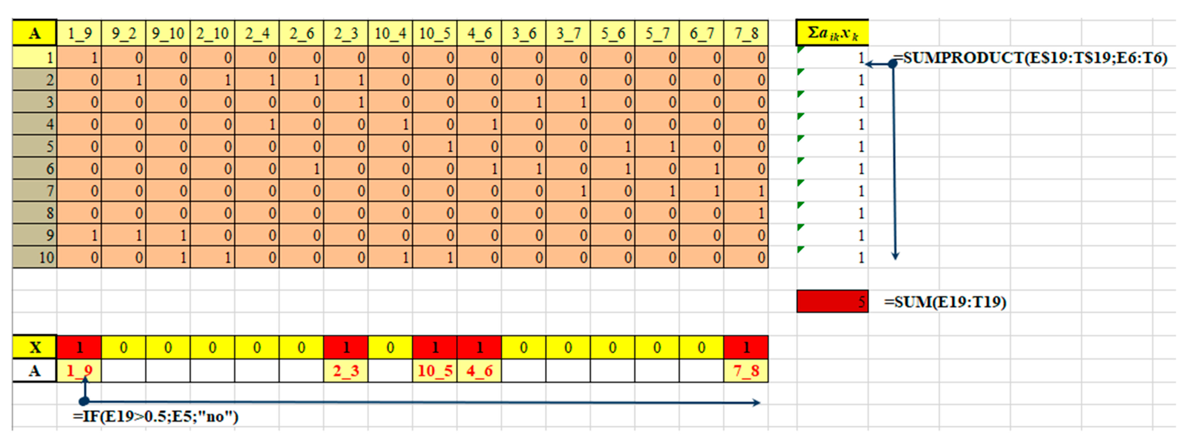
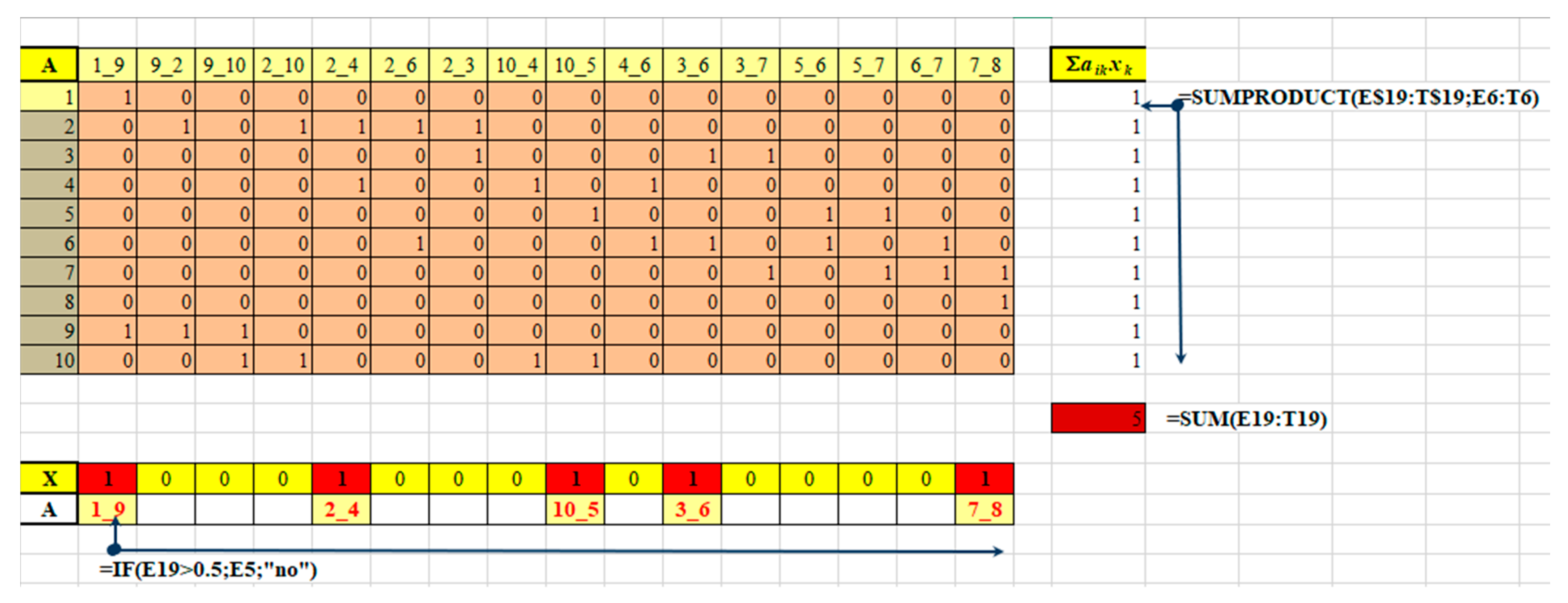
3.5. Maximum Matching (Independent Edge Set, Edge Packing) Problem

An edge packing, otherwise known as a matching, is a set of pairwise non-adjacent edges in a graph. Otherwise, an edge subset U* ⊂ U is called a matching in graph G(V,U) if no vertex v_i ∈ V is incident to more than one edge u_j ∈ U*. A maximum matching (also known as maximum-cardinality matching/edge packing) is a matching containing the largest possible number of edges [37].

Maximum matching problems occur when a group of people, a set of devices/premises, or their combinations are to be divided into pairs by the possibility or necessity of joint work. If each edge means the possibility or necessity of joint work or use, the problem is reduced to the creation of the largest possible number of workable pairs, i.e., non-adjacent edges (maximum matching). If the pairing provides different efficiency (performance, speed of information transfer, probability of error or risk), a weight corresponding to this efficiency is assigned to the edge, and the problem is reduced to determining the maximum weighted matching.

Denoting by x_k the edges of the graph included in the matching of graph G(V,U) with N vertices and T edges and using as before the extended incidence matrix A = {a_ik} to describe the structure of the initial graph, we obtain, via analogy with the previous cases, a mathematical model of the problem on finding the maximum matching of the graph as:

$$\begin{array}{c}\mathrm{X}=\left\{{\mathrm{x}}_{\mathrm{k}}\right\}, \mathrm{k}=\overline{1,\mathrm{T},} {\mathrm{x}}_{\mathrm{k}}=0\vee 1\\ \forall \mathrm{i}, \mathrm{k}=\overline{1,\mathrm{N}} {\displaystyle {\displaystyle \sum }_{\mathrm{k}=1}^{\mathrm{T}}}{\mathrm{a}}_{\mathrm{ik}}{\mathrm{x}}_{\mathrm{k}}\le 1\\ {\displaystyle {\displaystyle \sum }_{\mathrm{k}=1}^{\mathrm{T}}}{\mathrm{x}}_{\mathrm{k}}\to \max \end{array}$$

(8)

Similarly to MVC problem model (6), the model (8) is a BLP model. Applying the built-in Excel function SUMPRODUCT(array1, array2, … [array_n]) to implement the constraint ${\displaystyle \sum }_{\mathrm{k}=1}^{\mathrm{T}}{\mathrm{a}}_{\mathrm{ik}}{\mathrm{x}}_{\mathrm{k}}\le 1$, a spreadsheet model reflecting (8) takes form shown in

Table 7. MS Excel spreadsheet model of the maximum matching problem for graph G₂ (Figure 3) as a Boolean linear programming problem based on the model (8).

Cells	Formulas or Initial Values	Model Component
V6:V15	0	Vector of unknowns X = {xk}, corresponding to graph G2 edges. After performing the solution search procedure xk take values 0∨1; where 1 refers to edges included in maximum matching
E6:T15	0	The incidence matrix of the original graph G2
E20	=SUMPRODUCT(E6:E15;$V6:$V15), extended to F20:T20	Number of edges common to each vertex of the graph, ${\displaystyle \sum }_{\mathrm{k}=1}^{\mathrm{T}}{\mathrm{a}}_{\mathrm{ik}}{\mathrm{x}}_{\mathrm{k}}$
V17	SUM(E19:T19)	Objective function: matching number $\mathrm{F}={\displaystyle \sum }_{\mathrm{k}=1}^{\mathrm{T}}{\mathrm{x}}_{\mathrm{k}}\to \max$

and

Table 8. MS Excel spreadsheet model of the maximum matching problem constraints for graph G₂ (Figure 3) based on the model (8).

Constraint	Constraint Content
E19:T19=binary	The Boolean character of variables in the matrix of unknowns X, ${\mathrm{x}}_{\mathrm{k}}=0\vee 1$
$V$6:$V$15=<1	The requirement to have no common vertices for edges included in G2 matching.

and Figure 8.

Table 7 and Table 8 show that all model functions are linear. Transferring the model to the Solver dialog box, setting the optimization criterion to maximum, and choosing the simplex search method, we almost immediately obtain the solution {1_9, 2_3, 10_5, 4_6, 7_8} (Figure 8). This is one of the maximum independent edge sets in graph G₂.

Applying additional constraints either on the including or excluding of certain edges in maximum matching, other variants of the maximum independent edge sets can be obtained, in particular {1_9, 2_4, 10_5, 3_6, 7_8} and {1_9, 2_3, 10_4, 5_6, 7_8} with the same matching number of 5.

3.6. Maximum Weighted Independent Set (Maximum Weighted Matching, MVM) Problem

The problem differs from the previous one in requiring to maximize not the number of edges in a matching, but its cost under the assumption that each k-th edge has a certain cost (weight) c_k. The model of this problem differs from the previous one, presented by (8), only by the objective function that takes the form of $\mathrm{F}={\displaystyle \sum }_{\mathrm{k}=1}^{\mathrm{T}}{\mathrm{c}}_{\mathrm{k}}{\mathrm{x}}_{\mathrm{k}}\to \max$, which necessitates introducing into the spreadsheet model a one-dimensional array of the same size as the array of unknowns containing values (weights) of all T edges c_k. After placing this array in cells E18:T18, the objective function formula in cell V17 changes to SUMPRODUCT(E18:T18; E19:T19). Other model elements remain corresponding Table 7 and Table 8. After transferring the problem model to the Solver dialog box and running the simplex method, we obtain the solution MVM = {9_2, 10_4, 3_7, 5_6}. The number of edges in it is less than the previously obtained matching number for maximum matching (4 vs. 5), though the total cost of them is the largest possible. If the number of edges in matching is to be kept maximum, an additional constraint ${\displaystyle \sum }_{\mathrm{k}=1}^{\mathrm{T}}{\mathrm{a}}_{\mathrm{ik}}{\mathrm{x}}_{\mathrm{k}}=5$ is to be introduced as V16 = 5. The obtained solution {1_9, 2_4, 10_5, 3_6, 7_8} provides a total cost of only 37 < 39.

3.7. Minimum Line Cover (MLC) Problem

Line cover (edge cover) of a graph G(V,U) is such a subset of its edges U* ⊆ U that all vertices V = {v_i} are incident to at least one edge belonging to this subset U*. To solve the problem of minimum line/edge cover (MLC, MEC) means to determine the smallest number of edges sufficient to cover all vertices of the graph [37].

Denoting by x_k the graph edges included in the edge cover of graph G(V,U) with N vertices and T edges and using, as before, the extended incidence matrix A = {a_ik} to define the structure of the original graph G, similarly to the previous cases, we obtain a mathematical model of the MLC problem as:

$$\begin{array}{c}\mathrm{X}=\left\{{\mathrm{x}}_{\mathrm{k}}\right\}, \mathrm{k}=\overline{1,\mathrm{T},} {\mathrm{x}}_{\mathrm{k}}=0\vee 1\\ \forall i, k=\overline{1,N} {\displaystyle {\displaystyle \sum }_{k=1}^T}{a}_{\mathit{ik}}{x}_k\ge 1\\ {\displaystyle {\displaystyle \sum }_{k=1}^T}{x}_k\to min\end{array}$$

(9)

Similarly to previous problem models (6–8), model (9) appears to be a BLP model. Applying the built-in Excel function SUMPRODUCT to implement the constraint ${\displaystyle \sum }_{\mathrm{k}=1}^{\mathrm{T}}{\mathrm{a}}_{\mathrm{ik}}{\mathrm{x}}_{\mathrm{k}}\ge 1$, a spreadsheet model reflecting (9) takes the form shown in Figure 9 and

Table 9. MS Excel spreadsheet model of the minimum line cover problem for graph G₂ (Figure 3) as a BLP problem (8).

Cells	Formulas or Initial Values	Model Component
E19:T19	0	Vector of unknowns X = {xk}, corresponding to graph G2 edges. After performing the solution search procedure xk takes values 0∨1; 1 refers to edges included in MLC
E6:T15	0∧1	Incidence matrix of the original graph G2
V6	=SUMPRODUCT(E$19:T$19;E6:T6), extended to V7:V15	Number of edges covering each vertex of the graph, ${\displaystyle \sum }_{\mathrm{k}=1}^{\mathrm{T}}{\mathrm{a}}_{\mathrm{ik}}{\mathrm{x}}_{\mathrm{k}}$
V17	SUM(E19:T19)	Objective function: edge cover number of graph G2 (number of edges in MLC) $\mathrm{F}={\displaystyle \sum }_{\mathrm{k}=1}^{\mathrm{T}}{\mathrm{x}}_{\mathrm{k}}\to \min$ equal to the number of cells with value 1 in the range E19:T19, i.e., ones (xk = 1) in vector X

and

Table 10. MS Excel spreadsheet model of minimum line cover problem constraints for graph G₂ (Figure 3) based on (8).

Constraint	Constraint Content
E19:T19=binary	The Boolean character of variables in the matrix of unknowns X, ${\mathrm{x}}_{\mathrm{k}}=0\vee 1$
$V$6:$V$15>=1	The requirement to cover every vertex of graph G2 by at least one of the edges u ∈ U* belonging to the MLC

.

As Table 7 and Table 8 show, all model functions are linear. Transferring the model to the Solver dialog box, setting the optimization criterion to minimum and choosing the simplex search method, we almost immediately obtain the solution MLC = {1_9, 2_4, 10_5, 3_6, 7_8} (Figure 9), which is one of the G₂ minimum line covers.

Using additional constraints on the inclusion/exclusion of a certain edge, (e.g., consequently setting x_k = 0 for determined MLC edges), we get two more MLC sets ({1_9, 2_3, 10_5, 4_6, 7_8}, {1_9, 2_3, 10_4, 5_6, 7_8}) with the same cover number of 5.

3.8. Minimum Weighted Line Cover (MWLC) Problem

The problem differs from the previous one by aiming to minimize not the number of edges in line cover, but the MLC total cost assuming that each k-th edge has a certain cost (weight) c_k. Thus, the model of this problem will differ from the previous one only in the objective function $\mathrm{F}={\displaystyle \sum }_{\mathrm{k}=1}^{\mathrm{T}}{\mathrm{c}}_{\mathrm{k}}{\mathrm{x}}_{\mathrm{k}}\to \min$. Therefore, a new one-dimensional array C containing the edge costs (weights) c_k, $\mathrm{k}=\overline{1,\mathrm{T}}$ is to be introduced into the spreadsheet model. After placing this array in cells E18:T18, the objective function formula in cell V17 changes to SUMPRODUCT(E18:T18; E19:T19). Other elements of the problem model stay as they are in Table 9 and Table 10. Transferring the model to the Solver dialog box with setting the optimization criterion to minimum and choosing the simplex search method, we almost immediately obtain the solution MWLC= {1_9, 9_10, 2_3, 4_6, 5_7, 7_8}, in which the number of edges exceeds that previously obtained for MLC (6 vs. 5) (Figure 9), though the total cost of them is the smallest possible. If the number of edges in line cover is to be kept minimal, an additional constraint ${\displaystyle \sum }_{\mathrm{k}=1}^{\mathrm{T}}{\mathrm{a}}_{\mathrm{ik}}{\mathrm{x}}_{\mathrm{k}}=5$ is to be introduced similar to that described for maximum weighted matching problem.

3.9. Maximum Clique Problem

As shown above, the maximum clique in graph G can be found as the maximum independent set in the graph G** complement to G. The adjacency matrix M* of the complement graph G** can be easily obtained in Excel by subtracting 1 from each element of the adjacency matrix M of the original graph, with further multiplying it by −1 using the “Special Paste” operations with options “subtract” and “multiply”. Then, it is enough to construct the incidence matrix of the complement graph and solve the MVC problem or the maximum independent set problem. The maximum independent vertex set on graph G** will give the largest clique in graph G.

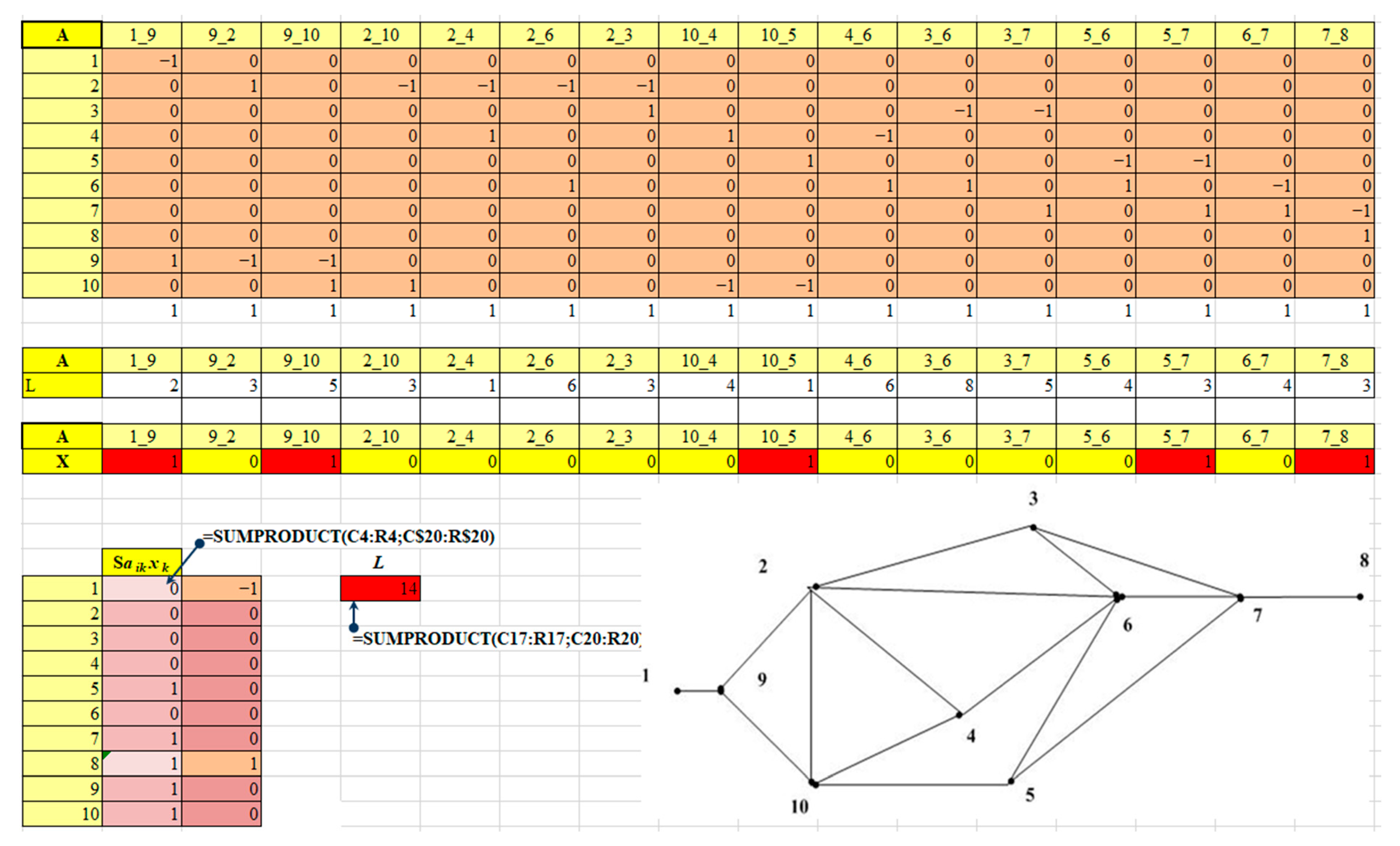
3.10. Shortest Path Problem

A model of this problem can be easily obtained based on the model for minimal edge cover of a graph by denoting by x_k the edges of the graph included in the minimal path between vertices v_l and v_m of the graph G(V,U) with N vertices and T edges and employing, as before, the extended incidence matrix A = {a_ik} of the graph to set the structure of the original graph. Similarly to the previous cases, we obtain a mathematical model of the minimal path problem as follows:

$$\mathrm{X}=\left\{{\mathrm{x}}_{\mathrm{k}}\right\}, \begin{array}{cc}\mathrm{k}=\overline{1,\mathrm{T},}& {\mathrm{x}}_{\mathrm{k}}=0\vee 1\end{array}$$

(10)

$$\begin{array}{c}\forall \mathrm{i}, \mathrm{i}=\mathrm{l}; \mathrm{i}=\mathrm{m}; \mathrm{k}=\overline{1,\mathrm{N}}; {\displaystyle {\displaystyle \sum }_{\mathrm{k}=1}^{\mathrm{T}}}{\mathrm{a}}_{\mathrm{ik}}{\mathrm{x}}_{\mathrm{k}}=0\\ \mathrm{i}=\mathrm{l}; \mathrm{k}=\overline{1,\mathrm{N}}; {\displaystyle {\displaystyle \sum }_{\mathrm{k}=1}^{\mathrm{T}}}{\mathrm{a}}_{\mathrm{ik}}{\mathrm{x}}_{\mathrm{k}}={\displaystyle {\displaystyle \sum }_{\mathrm{k}=1}^{\mathrm{T}}}{\mathrm{a}}_{\mathrm{lk}}{\mathrm{x}}_{\mathrm{k}}=1\\ \mathrm{i}=\mathrm{m}; \mathrm{k}=\overline{1,\mathrm{N}}; {\displaystyle {\displaystyle \sum }_{\mathrm{k}=1}^{\mathrm{T}}}{\mathrm{a}}_{\mathrm{ik}}{\mathrm{x}}_{\mathrm{k}}={\displaystyle {\displaystyle \sum }_{\mathrm{k}=1}^{\mathrm{T}}}{\mathrm{a}}_{\mathrm{mk}}{\mathrm{x}}_{\mathrm{k}}=-1\end{array}$$

(11)

$${\displaystyle \sum }_{\mathrm{k}=1}^{\mathrm{T}}{\mathrm{x}}_{\mathrm{k}}{\mathrm{l}}_{\mathrm{k}}\to \min$$

(12)

where l_k is the length of the k-th edge.

A fundamental feature of this model is treating graph G(V,U) as a directed one, i.e., passing of each of the edges is possible only in one direction. That is what provides connectedness of the path between the given vertices of the graph by setting constraints (11) reflecting the pass-through character of all intermediate path vertices. If the graph is undirected, additional dummy edges of opposite direction are introduced into the graph so that each real edge gets a multiple edge of opposite direction, and the incidence matrix is drawn for the resulting extended graph.

The form of a spreadsheet model of the problem of finding the shortest path between two vertices of a graph G₂ is shown in

Table 11. MS Excel spreadsheet model of the shortest path problem for directed graph G₂ (Figure 3) as a BLP problem (10)–(12).

Cells	Formulas or Initial Values	Model Component
C20:R20	0	Vector of unknowns X = {xk}, corresponding to graph G2 edges. After performing the solution search procedure xk takes values 0∨1; 1 refers to edges included in the shortest path from vl to vm; l = 1; m = 10
C4:R13	0∧1	Incidence matrix of the original graph G2
C17:R17	Numerical values	Lengths of graph edges (lk is the k-th edge length; cell C17 contains the length of the edge x1 ∈ X (cell C20); cell D17 contains the length of the edge x2 ∈ X (cell D20) etc.)
C25	=SUMPRODUCT(C4:R4;C$20:R$20), extended to C26:C34	${\displaystyle \sum }_{\mathrm{k}=1}^{\mathrm{T}}{\mathrm{a}}_{\mathrm{ik}}{\mathrm{x}}_{\mathrm{k}}$—sum of values in the row of the graph incidence matrix; after performing the solution search procedure it should take the value of +1 for the initial vertex of the path, of −1 for the final one and 0 for the intermediate vertices considering their transitive nature
D25:D34	0∧1∧−1	Right hand side of equations (11): +1 for the initial vertex of the path, −1 for the final one and 0 for the intermediate ones
F25	=SUMPRODUCT (C17:R17;C20:R20)	Objective function: $\mathrm{F}={\displaystyle \sum }_{\mathrm{k}=1}^{\mathrm{T}}{\mathrm{x}}_{\mathrm{k}}{l}_k\to \min$: shortest path length between graph G2 vertices v1 and v10

.

All model functions (Table 11 and

Table 12. MS Excel spreadsheet model of the shortest path problem constraints for the directed graph G₂ (Figure 3) based on (10) and (11).

Constraint	Constraint Content
C20:R20=binary	The Boolean character of variables in the matrix of unknowns X, ${\mathrm{x}}_{\mathrm{k}}=0\vee 1$
$C$25:C$34=$D$25:D$34	Condition (11) providing connectedness of the route between chosen vertices (v1 and v10) of graph G2

) are linear; therefore, after transferring the model to the Solver dialog box, setting the optimization criterion to minimum and choosing the simplex search method, we almost immediately obtain the shortest path {1_9, 9_10, 10_5, 5_7, 7_8} with length L = 14 (Figure 10).

To find the minimal path between any other vertices of the graph, we have to assume one of them as initial and the other as final setting for them, ${\displaystyle \sum }_{\mathrm{k}=1}^{\mathrm{T}}{\mathrm{a}}_{\mathrm{ik}}{\mathrm{x}}_{\mathrm{k}}=1$ and ${\displaystyle \sum }_{\mathrm{k}=1}^{\mathrm{T}}{\mathrm{a}}_{\mathrm{ik}}{\mathrm{x}}_{\mathrm{k}}=-1$, respectively. All other vertices are considered intermediate ones with setting ${\displaystyle \sum }_{\mathrm{k}=1}^{\mathrm{T}}{\mathrm{a}}_{\mathrm{ik}}{\mathrm{x}}_{\mathrm{k}}=0$. Changes in the spreadsheet model and examples of obtained solutions are given in

Table 13. Examples of constraint setting when exploring the shortest path between different graph nodes and the solutions found.

Initial Vertex	Final Vertex	Constraint Cell Values										Lmin	Minimal Path
		D25	D26	D27	D28	D29	D30	D31	D32	D33	D34
1	8	−1							1			14	1_9, 9_10, 10_5, 5_7, 7_8
1	6	−1					1					11	1_9, 9_2, 2_6
2	7		−1					1				7	2_10, 10_5, 5_7
9	6						1			−1		9	9_2, 2_6

.

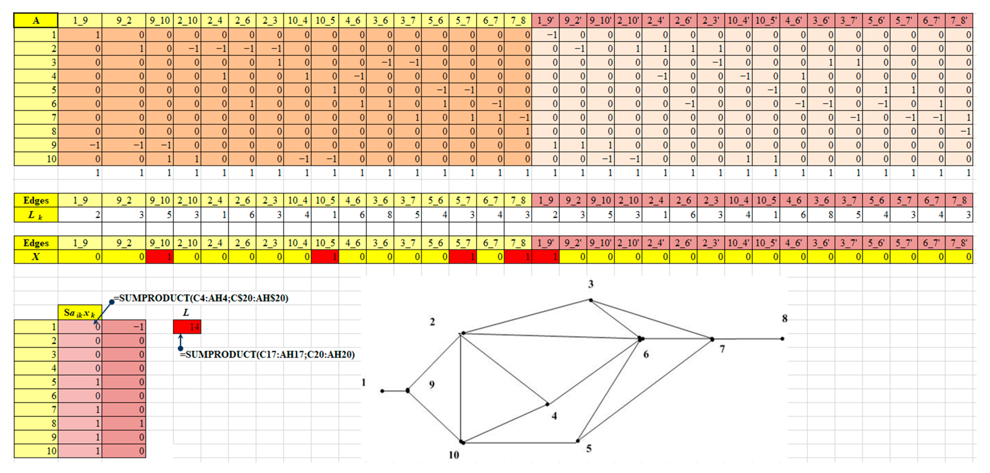
If the graph is undirected, it is necessary to introduce into it additional dummy edges multiple to each real edge of the graph and having the same length, but opposite direction. In this case, the incidence matrix on the Excel sheet is expanded twice by inserting its copy with inverted values, obtained by pasting a copy of the matrix into neighboring cells with further multiplication by −1 (Paste Special option). The size of the vector of unknowns as well as the associated set of cells and the set of cells with lengths of edges are also doubled. The expansion of the matrices is reflected in changing the formulas of the objective function and constraints (Figure 11).

If it is necessary to find not a minimum, but a maximum path on the graph, as is the case of calculating the work duration by the critical path (CP) network method, one needs to change the optimality criterion from minimum to maximum. Solution CP = {1_9, 9_2, 2_10, 10_4, 4_6, 6_7, 7_8} and maximum path length L = 25 are obtained almost instantly.

4. Discussion and Conclusions

Solver is a optimization tool that has several advantages over other computer programs [44]. For example:

-

It is affordable and easy to use. Solver is integrated into MS Excel, which is a widely used and familiar software for many users.

-

It is quick and flexible. The simplex method is a fast and efficient algorithm that can handle problems with many variables and constraints. Additionally, it is a flexible tool that can handle a wide range of linear programming problems, including problems with nonlinear constraints, integer variables, and nonlinear objective functions.

-

It is interactive. Solver has an interactive interface that allows users to modify the problem formulation and constraints easily and see the impact of these changes on the optimal solution.

It is worth noting that Solver has some limitations. For example, it may not be suitable for large-scale problems that require more sophisticated optimization algorithms or specialized software [45].

Representation of extreme problems on graphs as Boolean linear programming problems and spreadsheet models suggested for them, provide an opportunity to set and solve a wide range of practical problems in various fields, from marketing, logistics, and management to design of transport and telecommunication networks, optimization of component allocation and PCB tracing, which are reducible to extreme problems on graphs with quite large strength. The main advantage of the suggested approach is the unified setting of a graph by its expanded incidence matrix and of a vector of unknowns by the vector of binary variables associated with vertices or edges of the sought parts of the graph, which makes it possible on the basis of actually just two templates to create spreadsheet models of a number of extreme problems on graphs (minimum vertex and edge cover problems, maximum independent set, maximum matching and clique, critical path problems), differing only in the extremum type and constraint sign.

The specificity of MS Excel built-in functions and MS Excel Solver options provide modeling and solving of these problems as linear programming problems using the simplex method without programming tools; the acceptable graph strength is limited by the number of graph vertices/edges compared to the maximum possible number of Boolean variables for MS Excel Solver (from 100 to 400 in different versions of MS Excel Solver). The obtained models and procedures for solving the considered types of problems can be efficiently applied when solving practical tasks in various fields.