Article

Characterisation of Composite Materials for Wind Turbines Using Frequency Modulated Continuous Wave Sensing

1
James Watt School of Engineering, University of Glasgow, Glasgow G12 8QQ, UK
2
The School of Engineering and Physical Sciences, Heriot Watt University, Edinburgh EH14 4AS, UK
*
Author to whom correspondence should be addressed.
J. Compos. Sci. 2023, 7(2), 75; https://doi.org/10.3390/jcs7020075
Submission received: 8 December 2022 / Revised: 25 January 2023 / Accepted: 30 January 2023 / Published: 10 February 2023
(This article belongs to the Special Issue Machine Learning in Composites)

Abstract

:
Wind turbine blades (WTBs) are critical sub-systems consisting of composite multi-layer material structures. WTB inspection is a complex and labour intensive process, and failure of it can lead to substantial energy and economic losses to asset owners. In this paper, we proposed a novel non-destructive evaluation method for blade composite materials, which employs Frequency Modulated Continuous Wave (FMCW) radar, robotics and machine learning (ML) analytics. We show that using FMCW raster scan data, our ML algorithms (SVM, BP, Decision Tree and Naïve Bayes) can distinguish different types of composite materials with accuracy of over 97.5%. The best performance is achieved by SVM algorithms, with 94.3% accuracy. Furthermore, the proposed method can also achieve solid results for detecting surface defect: interlaminar porosity with 80% accuracy overall. In particular, the SVM classifier shows highest accuracy of 92.5% to 98.9%. We also show the ability to detect air voids of 1mm differences within the composite material WT structure with 94.1% accuracy performance using SVM, and 84.5% using Naïve Bayes. Lastly, we create a digital twin of the physical composite sample to support the integration and qualitative analysis of the FMCW data with respect to composite sample characteristics. The proposed method explores a new sensing modality for non-contact surface and subsurface for composite materials, and offer insights for developing alternative, more cost-effective inspection and maintenance regimes.

1. Introduction

Among the different renewable energy generation sources, wind power plays an increasingly important role to global clean power. During the last two decades, global wind power capacity has grown at a rapid pace. Record growth was seen in 2020 where the wind power industry installed 93GW of new capacity, an unprecedented 53% year-on-year increase [1]. As this promising sector grows, reduction in Operational and Maintenance (O&M) costs, increased reliability and resilience of wind turbine systems becomes crucial.
The O&M costs of wind turbines represent 25% to 30% of overall energy generation cost [2], where WTB are generally considered the most critical asset [3], its manufacturing cost accounts for 15–20% of each wind turbine installation cost [4]. The increasing demand for renewable energy supply also calls for larger and lower-cost WT blades, therefore, modern WTB typically employ composite materials [4], such as glass fibre reinforced polymer (GFRP) and carbon fiber reinforced polymer (CFRP). These composite materials are cost-effective options for asset owners with the features of high stiffness and light weight [5]. but also face potential defects such as delamination and debonding which undermines its reliability. This issue becomes increasingly important as longer and wider blades ranging from 20 to 100 m are manufactured to enable more energy capture, which also implies heavier load levels which affects the operational safety of WTBs [6,7].
Failure or damage to WT blades can also lead to substantial economic losses [8]. WT blades are subject to both manufacturing defects and damage from harsh operating environment, such as ultraviolet radiation, wind gusts, moisture absorption, fatigue, ice accumulation and lightning strikes etc. [9,10]. Meanwhile, when subjected to structural testing, damage such as cracks may occur to the composite material and adhesive interface of WT blades. Full scale testing may also result in delamination and debonding of the turbine structure [11]. Additional difficulty for Asset Management(AM) of WT blade is data availability where detailed documentation and data on the range and extent of damages are generally unavailable.
Thus, once a WTB has been installed, it is essential to perform non-destructive evaluation (NDE) techniques to prevent failure [12]. Existing NDE methods tested and used for WTB include visual inspection, sonic and ultrasonic, thermography, and electromagnetic. These methods have been reviewed in detail by researchers over the years as in [13,14,15] showing different strengths but als limitations. For example, visual inspections can be ideal for examining surface defects yet unable to provide inner-structure evaluations [16,17], ultrasonic sensing may have lower computation cost but face sound attenuation and scattering concerns [18], and may require complicated equipment set-up [19]. Strain measurement provides in-service monitoring but is difficult to retro-fit [20], while AE sensor systems are sensitivity to noise [13]. The need for an NDE method that is resilient, low-cost, and easy to implement is crucial for addressing the challenges associated with monitoring WTBs. Such a method would improve the overall efficiency and effectiveness of WTB management.
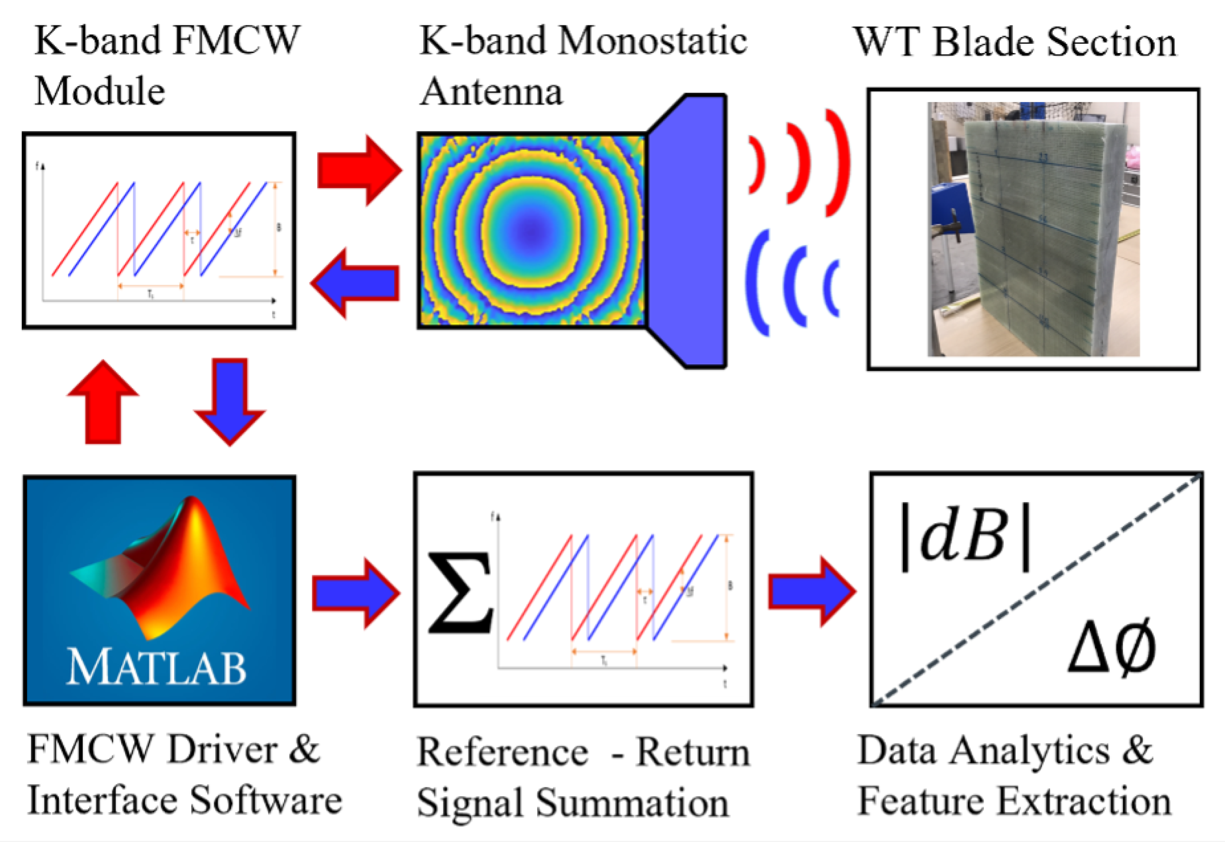
In this paper, we present a novel NDE method using a patented Frequency Modulated Continuous Wave (FMCW) radar technology for composite material and defect characterization of WTBs. Specifically, we integrate the FMCW sensor onto a robotic manipulator for automated raster scanning and collect data on different WTB samples, and build a data library. Machine learning algorithms are then trained with pre-processed data of WTB, and showed good performance in characterizing WTBs with different physical features(with 98.5% prediction accuracy). We further demonstrate the ability to use the proposed NDE method to capture WTB surface manufacturing defects (i.e., interlaminar porosity and sub-surface air voids with 94.1% prediction accuracy). We demonstrate the encouraging potential of FMCW in capturing WT blade physical and defect information, and the automation of this light weight, low power, and tunable technology for advancing inspection procedures in NDE of composites. Finally, we present a Digital Twin (DT) of the WT blade. This DT acts as an Asset Integrity Dashboard (AID), which aims to display return signal data from FMCW experiments in a more intuitive fashion for those not familiar with the technology and how to interpret the results.
The remainder of this paper is structured as follows; Section 2 introduces a literature review of NDE methods for WTBs. Section 3 brings the FMCW radar background, dielectric theory and our experiment settings. Section 4 and Section 5 describes the overall machine learning methodology, data acquisition procedures and machine learning modelling for WT defect detection and associated results. 
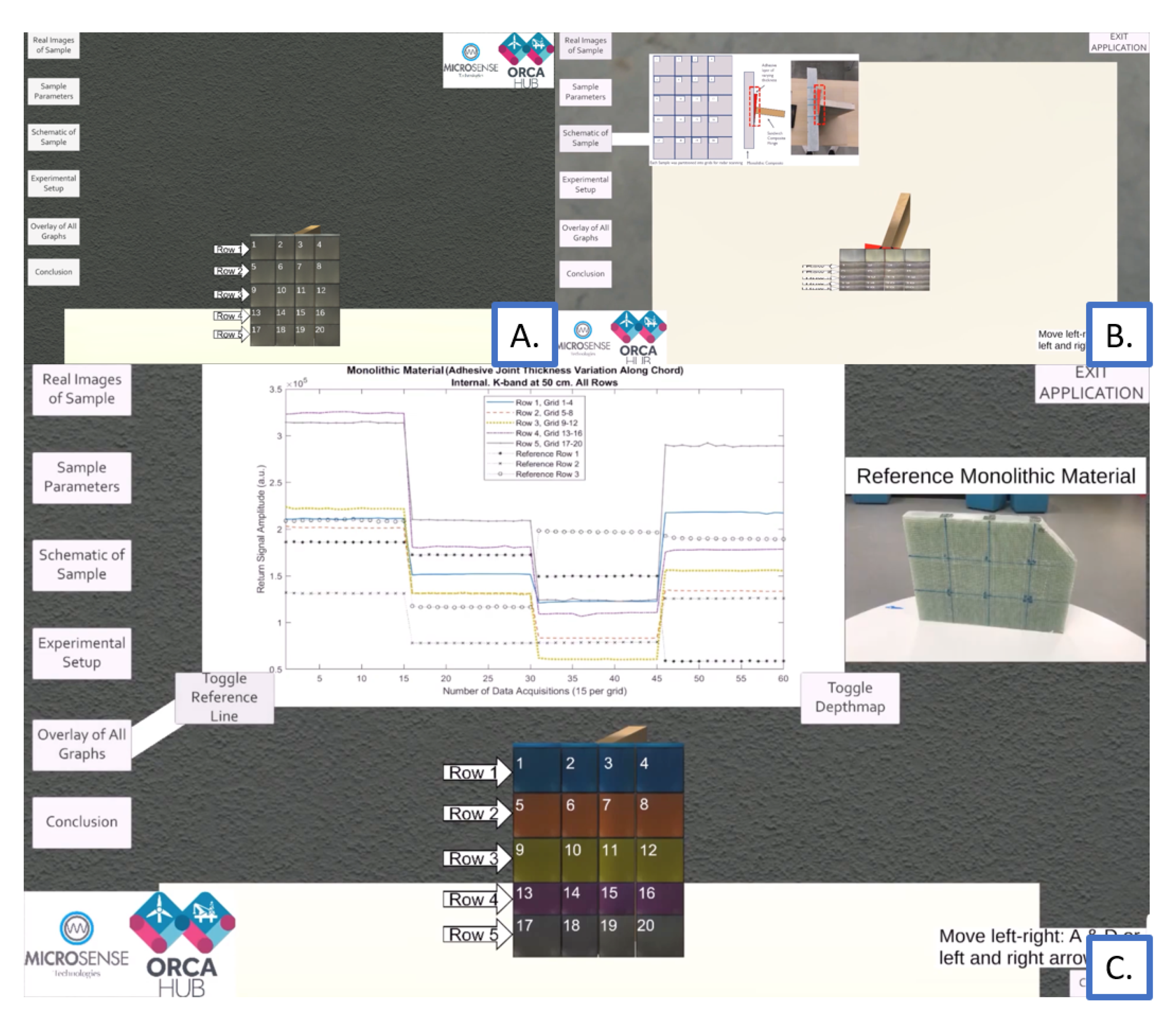
Section 6 presents the visualisation of the WT inspection in a DT. Section 7 provides the future work and discussion and lastly, Section 8 brings the final conclusion.

2. Literature Review of NDE Techniques for WTBs

Most modern WT blades employ glass fiber reinforced polymer (GFRP) and, in some cases, carbon fiber reinforced polymer (CFRP) are also increasingly used [6,7]. These composite materials form the sandwich structure of WT blades, which features high bending stiffness, high buckling resistance while remaining light-weight.
Growing demand for pollution-free electricity in the global energy transition has fuelled increasing interest in WT blade monitoring and fault diagnosis. Failure or damage to WT blades may occur during manufacturing or continuous operation [21,22]. For example, ultraviolet radiation, wind gusts, ice accumulation or lightning strikes etc [9,10]. Meanwhile, when subjected to structural testing, damage such as cracks may occur to the composite material and adhesive interface of WT blades. Full scale testing may also result in delamination and debonding of the turbine structure, which are common modes of WT blade damage [11]. While it is economically beneficial to identify damages early, WT blade composite structure has made fault diagnosis of the asset at early stage challenging [6,23,24,25]. This characteristic poses significant monitoring cost in WT blades and bring challenges to damage investigation, diagnostics, and maintenance strategies [6]. Additional difficulty for Asset Management(AM) of WT blade is data availability where detailed documentation and data on the range and extent of damages are generally unavailable.
Given the increasing number of distributed installations further from the shoreline, modern wind turbines and WTBs face harsher and more complex operating environments. The effective utilisation of wind turbine assets such as wind-turbine blades requires comprehensive and detailed SHM to maintain asset structural integrity during operation. To support SHM, NDE are often conducted through different techniques such as manual inspection, strain measurement, acoustic emission (AE) testing, ultrasound testing etc. In this section, we will present a review and discussion of the latest NDE methods and their use for WTB. Visual inspections can be fast and inexpensive for examining external surface faults of WTBs [16]. However, visual inspections often require good sight of the object which may pose safety concerns to the inspector [13], and are subject to human skills and interpretation limitations [24], and may be time-consuming for large objects. Recent development of automated camera systems can help reduce human labour hazards [16], but remains unable to identify inner structure damages.
Acoustic emission method is a physical contact-based, vibration-based fault detection technique for WT blades. It is widely employed for detecting elastic stress waves that represent accelerated fatigue or cracks, and locating such faults in composite materials and WTBs [26,27,28]. However, AE sensors needs to be embedded or mounted which can be expensive to asset owners, and due to its high sensitivity, noise disturbance may also mask the fault signals collected by AE sensors [15,22]. Therefore, when considering AE for fault detection, AE sensors need to be placed near the location of blade damage to be effective [11], when fault location is unobservable from the surface, multiple AE sensors need to be placed on different points of the blade. There are also concerns with accurate mapping of AE data with specific damage mechanisms [29], and the need to use other NDE methods for result verification [30].
Strain measurement is another example of contact-based NDE. For example, Fibre Optic Bragg Grating (FBG) sensors can be used as strain measuring devices to provide continuous load data during WT blade operation [20], while microbending optical fibre sensors were shown to be useful for detection of cracks in WT blade adhesive joints [31]. Despite their effectiveness in damage detection tasks, optical fibre sensors require complex and expensive configurations, which limits their usefulness for efficiency and economic reasons.
Ultrasonic testing evaluation systems use high frequency sound waves to penetrate composite materials and identify characteristics of internal defects, such as crack location, size and orientation [8,32]. It is suggested that this method is suitable for verifying quality of lamination between layers of composite materials for WT blades [33,34]. The limitation in ultrasonic technique lies in its dependence on a water or gel couplant.
Alternative to contact-based NDE methods, electromagnetic NDE does not require physical contact with the blade and can penetrate nonconductive materials and provide the spectral response of the material [35,36]. Examples of this method include: eddy current, radio frequency eddy-current, and microwave. Eddy current can be used for evaluating CFRP [26] and metallic composites [37], and may be used for delamination detection [35,38]. Radio frequency eddy-current is also applicable to CFRP. As reviewed in [39], it is typically employed for misalignments, polymer degradation and layer orientation. Microwave technique using electromagnetic radiation with millimeter wave spectrum, has shown some potential in detecting GFRP composite material faults such as wrinkles and flat bottom holes [13,40,41]. Laser ultrasonic systems can also provide a contactless imaging solution for rotating blade fault such as debonding and delamination but requires complex system setting and faces low sensitivity issues [13,42]. Other non-contact NDE methods for composites such as optical or non-optical thermography are often time-consuming to use, especially for thick materials, requiring material to be conductive, or have complex system [43,44]. A comparable summary of these NDE methods is illustrated in Table 1.
The above table summarizes existing techniques for WTB NDE inspections and monitoring. As highlighted in the table, there are still challenges which prohibit universal deployment of these inspection methods in real-world. For example, offshore operators may prefer sensing modality that doesn’t need a couplant, can operates without contact and even at a safe distance from the material under test. In addition, being able to operate reliably in a wide range of weather conditions could also be a desirable factor. As such, developing a technique with minimal contact and rapid inspections would add value for asset owners. This could potentially reduce the required manpower currently required during visual inspection [46] and allow for UAVs to complete a more accurate/compliment inspection due to the inclusion of subsurface analysis [47].
In this paper, we present a unique method of NDE for surface and sub-surface diagnostics of composite material in WTB samples by utilizing a patented Frequency Modulated Continuous Wave (FMCW) radar technology. This compact sensing technology is electromagnetic, non-contact, light weight, low power, robust and tunable, providing viable payload for autonomous, as well as resident, inspection systems [48]. Previous work of FMCW sensing for material analysis as an inspection tool for the K-band and X-band has been reviewed and summarized by the authors [49]. FMCW has recently been applied as a system for NDE of WTBs for studying the delamination, cracks, water ingress and composite material characterisation [50,51]. Other applications include analysis of dynamic load deformation in geomaterials for sample failure prediction [52], detecting corrosion and corrosion precursors [53] and for the analysis of core contents of partially fluid-saturated materials [54,55]. The technology was also shown to support localization in opaque environments and for safety applications, wherein the detection of people concealed by walls can provide forewarning of people about to enter the mission space of an autonomous robotic platform [56,57,58,59].

3. FMCW Sensing Background

3.1. FMCW and Dielectric Theory

FMCW represents a “continuous wave” sweep, where the output frequency is modulated to create a saw-tooth output. The difference in frequency between the emitted and return signals is determined by summing output and input waveforms to give a low frequency signal, which is then analyzed to infer the properties of an object in the Field Of View (FOV). This is termed the Intermediate Frequency (IF) signal of frequency Δ f . The determination of the IF signal is as follows [60]:
f R F o u t = f R F 0 + k f t
where 0 t T , f R F 0 (Hz) is the starting frequency, T(ms) is the chirp duration (frequency sweep duration), k f (Hz/s) is the sweep rate. The negative time of flight can be taken as a magnitude, allowing for the expression:
Δ f = B T 2 d c
where B(GHz) is the frequency sweep bandwidth, d(m) is the distance between the reflecting target and antenna and c(m/s) is the speed of light in the medium of propagation.
Due to the relationship expressed in Equation (2), the distance between the sensor and target is kept constant. Thereby, any signal variation can be attributed to the target surface intrinsic properties, as long as d is known. More in depth analysis of the FMCW radar theory can be found within Blanche et al., 2020 [51].
The dielectric theory processes for composite materials are governed by EM wave attenuation and dispersion, often termed “dielectric relaxation”. The frequency of the transmitted signal, which propagates to the material, is the key factor for the relaxation process. This results in oscillations, which dampen the signal at differing rates as a function of the component scale range [61]. Key features including surface and subsurface properties can be extracted from the return signal amplitudes via amplitude signal variations received at the antenna. Properties such as interfacial geometry, fluid content and type, surface contaminants and abundance of high permittivity minerals can affect the received amplitude [51]. Therefore, amplitude signal variations can be attributed to the intrinsic properties of the material and asset condition for a specific range. This can be characterised via contrasts in a predetermined baseline of a standard material sample. A full description of FMCW radar interaction between porous media partially saturated with fluids and internal geomaterial properties via non-invasive FMCW measurement is provided by Blanche et al. [51,55].

3.2. Radar Specification

The K-band radar module was connected directly to a Flann 21-240 Standard Gain Horn (SGH) antenna via a SMA/SMA connector rated to 26 GHz, with key operating parameters given in Table 2 [51,60]. Figure 1 provides a block diagram of the sensor setup and analytical workflow. Evaluation of the utilized Flann Microwave antenna shows it to have a peak amplitude spot size on the target of 36.4 mm radius at an antenna—target separation of 10 cm. Assuming a consistent near field divergence of 15 ° for the radiation pattern emitted from this antenna, the FOV for a target separation of 30 cm is 20 × 10 3 m 2 [51,60].
The FMCW radar sensor was configured in the following way as highlighted in Figure 2. This method allowed for surface and subsurface analysis of the material under test where MATLAB was utilised to initiate the continuous wave and collect data at the transceiver antenna.
The next two sections will explore the feasibility of FMCW and machine learning techniques in identifying variation physical properties of WTB composite structures, detection of different defects, and evaluation of defect severity.

4. WTB Composite Characterization Using Machine Learning and FMCW Data

This section summarizes the experimental and data acquisition procedure for WTB structure characterization. We do so by firstly building a data library via FMCW sensor onto a robotic manipulator for automated raster scanning and collect data from different WTB composite test samples with different composite types and diameter differentials. The data is preprocessed and then used to further explore the capability of data driven approaches. Different machine learning models are then trained to distinguish the composite material test samples, with key features extracted from the radar return signal amplitude (RSA).

4.1. Experiment Samples

Two monolithic and one sandwich composites samples have been used for the purpose of this study, as both types of composites are routinely used in WTB structures. The material and physical property is illustrated in Figure 3. The data collected from the FMCW radar sensor was taken from sandwich and monolithic composites which were manufactured by EDF R&D division as representative analogues which could include faults found on wind turbine blades. This was used to evaluate the capacity of the FMCW radar sensor NDE. The fabrication process of these types of WTB composite can be found in [23,62,63].

4.2. Robotic Integration and Data Collection

An automated raster scan was conducted via a robotic manipulator to obtain sufficient radar signals for each sample. During the scanning, the surface of the target sample was subdivided into a sequence of strips. Each strip was further divided into discrete small pixels for the FMCW sensor to aim and obtain the RSA. The return signal of each scan captures the material properties within the specific field of view across the whole sample surface. The objective was to collect enough radar signals from these evenly divided areas and to extract the common pattern, which can be used to represent this certain type of the composite material sample. We integrated the sensor with a robotic manipulator arm (UR3) [64] for an automatic raster scanning, to ensure smooth and consistent experiment conditions. The antenna was positioned so that the direction of Electromagnetic (EM) propagation was perpendicular to the blade surface. Firstly, the robot arm was manually positioned in free drive mode to face the pixel point at the top left corner of the target sample surface with a separation (e.g., 10 cm) distance between the target and the antenna tip. This point is where the first scan was taken. The robotic arm was programmed to move horizontally with a fixed step distance to scan the adjacent pixel point until reaching the pixel point on the top right corner of the surface of the blade. This action was repeated row by row until the full area of the target was scanned. For each target sample we also collected raster scan data with the radar at various distances from the surface(e.g., 10 cm, 15 cm and 20 cm) to ensure sufficient data for a richer training pool.

4.3. Machine Learning Modelling and Algorithms

In machine learning, classification refers to the ability of a model to assign instances to their correct groups. In the context of our case, this means to correctly output the type of composite sample when given radar RSA from a specific area of scanning. The process of machine learning classification modeling for the analysis of composite materials utilizing FMCW radar RSA data involves several steps(as illustrated in Figure 4). Firstly, the raw data are obtained through the method outlined in Section 4.2. The raw data are then subject to cleaning and normalization procedures, and are labeled accordingly. The dataset is then divided into two subsets, with the majority being allocated to the training dataset (75% of the total dataset) and the remaining portion allocated to the testing dataset (25% of the total dataset). This approach allows for the development of an accurate model through the training dataset, and the evaluation of its performance through the testing dataset.
After this data preparation process, we implement different machine learning algorithms using training dataset, which contain features of different inner composite structure and physical dimensions of WT blades, to train classification models.
Support Vector Machine, Bayesian Network, Decision Trees and Back Propagation network were firstly implemented to explore the capability of machine learning approaches for this multi class classification problem.

4.3.1. Support Vector Machines

Support Vector Machine (SVM) is a well-known and widely used classification model for finding a hyper-parameter that separates different groups of data and maximizes the margin between them using gradient descent [65]. In SVM, the computations of data points separation depend on different mathematical functions that are defined as the kernel. The function of the kernel is to take data as input and transform them into the required form.

4.3.2. Bayesian Method

Bayesian network [66] is a well-known probabilistic graphical model that represents a set of variables and their conditional dependencies via a Directed Acyclic Graph. As such, Bayesian network is a useful tool to visualize the probabilistic model for a domain, reviewing all relationships between random variables, and determining causal probabilities for scenarios given available evidence.

4.3.3. Back Propagation Neural Network

Artificial Neural Network (ANN) is also known as neural network or connection model. The ANN is a useful tool of mapping complex nonlinear relationships, and it also shows good robustness and fault tolerance when applied to an unfamiliar or unknown system. Back propagation (BP) network [67] is a multilayer feed forward network which originally runs error back propagation algorithm for training purposes. It is currently one of the most popular NN models in the field of signal image processing and classification.

4.3.4. Decision Trees

Decision trees [68] is a method widely used in machine learning. The goal of the tree model is to train a model that predicts the value of a target variable based on several input variables. It classifies testing samples by sorting them from the root to some leaf node in the tree, with the leaf node providing the classification to the example.

4.4. Data Analysis and Results

In this study, the classification model was trained using different forms of RSA data, e.g., the raw RSA data and processed data through different feature selection methods.

4.4.1. Training from Raw RSA Signal

The raw data obtained from the radar sensor are in the time domain with 1501 sampling points in 0.3 s. This occurs across a frequency sweep from 24–25.5 GHz, with an oscillating signal of an amplitude at approximately 103 digital units. The signal output from the FMCW sensor is the Intermediate Frequency (IF), the difference between the emitted and received signal and represents the time-of-flight data and the target interactions with the incident wave.
In this work, 600 raster scans from three different distances were conducted for each composite samples from turbine, therefore 600 raw signal data were collected for each class and each data point contains a vector with 1501 dimensions representing the time domain signal returned from the target. In this work, the Class 1, 2 and 3 refer to Composite material test sample No.1, No.2 and No.3. with order in Figure 3. It is notable that sample No.1 and No.2 shares the same monolithic composite structure but different thickness (2.5 mm), where sample No.3 is the sandwich blade with different material structure. The models were trained with 75% data from the raw data pool and tested with the remaining 25% data. When given a new observation from the testing data pool.
In this study, the Principal Component Analysis (PCA) [69] technique is also used for feature selection and dimensionality reduction, to further evaluate the capabilities of different models when given compressed observation data. In this work, nine primary components were generated to achieve the 95% explanation of the original variability. The overall accuracy of an algorithm in this study is calculated as the mean proportion of the correct output. The comparable results of the model performance trained from different dataset are shown in Table 3.

4.4.2. Training from Amplitude Data in Frequency Domain

In this study, post data processing was performed via Fast Fourier Transform (FFT), which transfers the time domain raw signal into the Frequency Domain (FD), from which amplitude extractions were analyzed and used for model training. Performing FFT transformations on the original datasets gives the spectral results, and with the special feature of the FMCW radar (the frequency of the signals changes over time), we can extract and learn the RSA in a range domain. For the FMCW radar in our study with a frequency span of 1.5 GHz, the resolution of the frequency bins corresponds to 0.1 m in air. This type of dataset contains the RSA which received from the reflections in every 0.1 m, after the EM propagation penetrates through the target sample. In our work, we explored the fusion of machine learning and spectral radar signals to extract key material properties of the testing samples for training our classification models. We also trained our models with selected FD data extracted within limited range (the lowest frequency responses containing the RSA in a 1m range from the antenna). The overall performance of our ML classification systems is shown in Table 4.

4.5. Results

The results demonstrate the capability of FMCW radar sensing for composite material characterization of WTBs. It also shows that machine learning approaches are able to provide robust data analyses from the FMCW RSA data. From Table 3, we see that the overall performance of all machine learning classifiers is satisfying, where SVM provides the best performance with 95% accuracy, and the Naïve Bayes has the lowest, but still acceptable, accuracy of 80.7%. Furthermore, it is notable that while Class 1 and Class 2 blades only differ slightly in thickness (3mm), the Class 3 blade differs from the two types in material structure. Due to these features, we would expect blades that have the same composite to have more similar radar RSA than those who do not. This expectation is realized in our model evaluation.
The results of Table 3 are also presented in a confusion matrix, also known as an confusion matrix to give a improved visualization of the performance of different algorithms. In the matrix, each cell shows the percentage of testing data from a given true class that is classified as a particular predicting class by the model. As shown in the confusion matrix in Figure 5, for all models, when given test data from Class 1 (or Class 2), incorrect outcomes are more frequently classified as Class 2 (Class 1) than Class 3. Overall, our machine learning model is still able to distinguish Class 1 and 2: the SVM model achieves very promising results with accuracy of 94.3% and 96.8%. Moreover, all of the models exhibit better performance when classifying samples with different material structure (given Class 3). This demonstrates the sensitivity of the FMCW, and the capability of these machine learning models to extract key features from the radar RSA. The results demonstrate the ability to detect minor inner characterisation differences of testing samples, this is an advantage that cannot be achieved with the current state of the art externally deployed NDE technologies for composite turbine blades.
The results also display the capability of machine learning models when trained with compressed raw RAS data (91% for the SVM, and 83.5% of the rest in average), this indicates the potential and flexibility for dealing with higher resolution signals (higher dimension of the training data) in the future. Furthermore, results in Table 4 demonstrate that most of the models will have improved performance when using extracted frequency/range domain RSA data as training data. All models can achieve an accuracy over 84.5%. In particular, SVM with polynomial kernel function reaching 98.5% accuracy, which demonstrates that the frequency domain data from FMCW reveals richer features and key characteristics about composite material physical properties. This could also benefit data-driven approaches for a more robust characteristic evaluation. We can also learn from Table 4 that machine learning models in our tests can still provide solid classification performance when trained using RSA signals with selected and limited range (1 m behind the antenna, with the scanned sample in the middle): the decision trees and SVM achieved an overall 88.6% and 92.9% accuracy, respectively.

5. Diagnostics on Manufacture Defects of WTB Composite

The previous section demonstrated that FMCW radar is sufficiently sensitive for inner integrity assessment. As such, in this subsection, we continue to explore its capability for WTB diagnostics of defect under surface and sub-surface, using samples with manufacturing defects.

5.1. Defective Samples

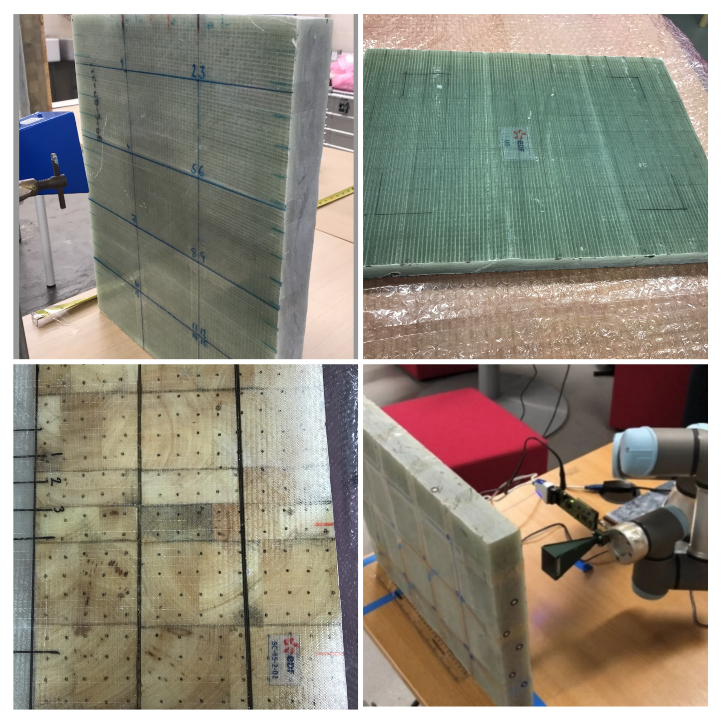
In this paper, we examine manufacturing defects of WTBs. We collected three composite materials samples used in WTB as for our analysis, two of which are sandwich composite samples and one monolith sample. The two sandwich composite (SC) samples have the same structure and composition and both contain manufacturing defects. Specifically, we examine a sub-surface defect known as air voids in balsa. The air voids in these two SC blades also differ in their sizes (as illustrated in Figure 6).
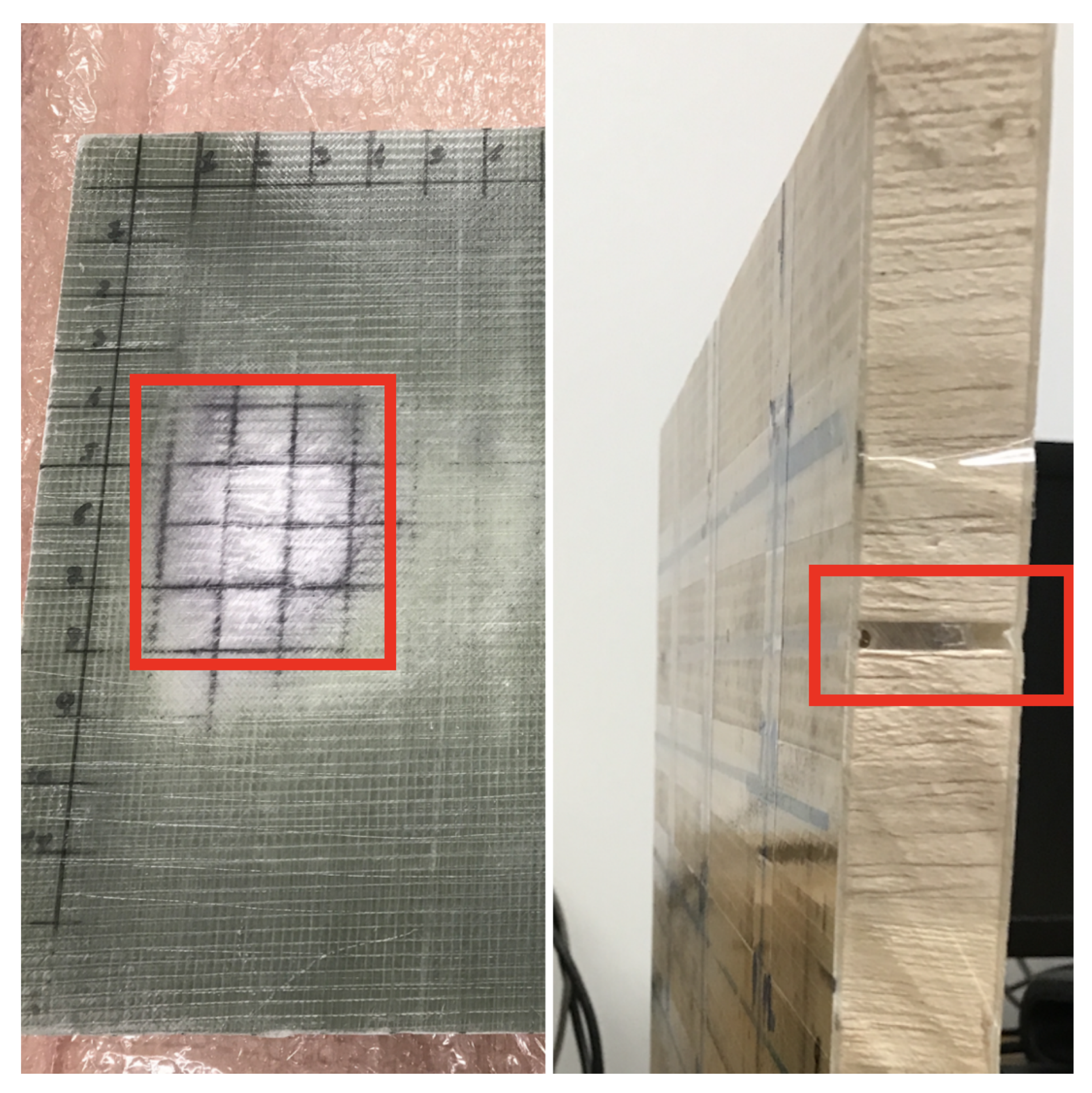
An additional type of defect we study is the interlaminar porosity (a visual representation is an area of white dry zone) which is manufacture defect on blade surface. For this purpose, we examine the monolithic composite (MC) sample. This MC sample is shown in the Figure 6 below with two notable dry zone areas. Specification of samples can be found in Table 5.

5.2. ML Modelling and Data Collection for Defect Detection

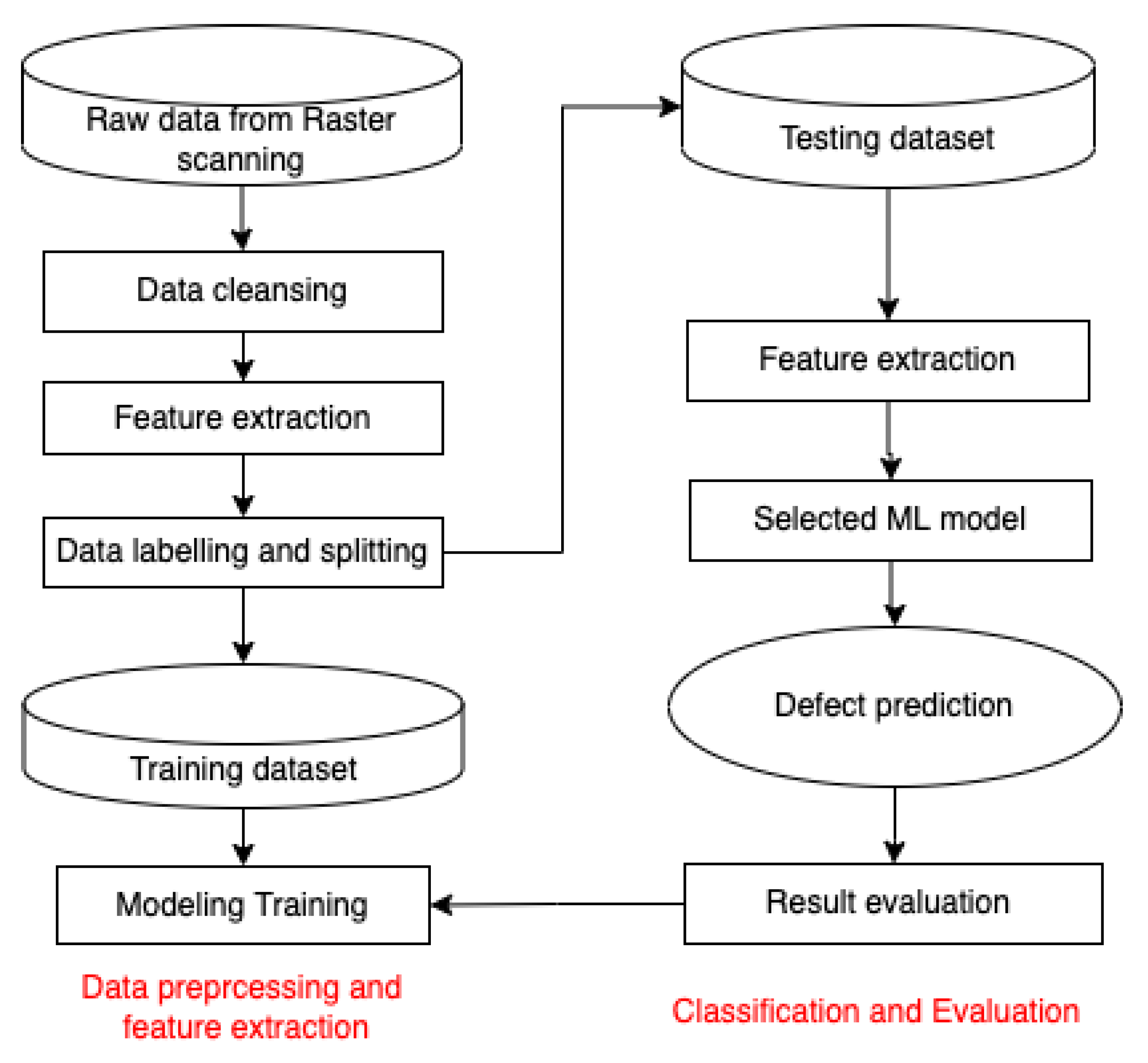
To achieve surface and sub-surface defect detection, we identify data collection requirements/process as follows: firstly, the type of data we needed must be able to represent different classes, i.e, areas with healthy surface/subsurface; areas containing both healthy and defective surface/subsurface, and finally defect-only areas. After this data collection process, we trained different machine learning classification models to identify whether the targeted area contains surface or sub-surface defects.
We conduct raster scans using the same equipment setup described in 
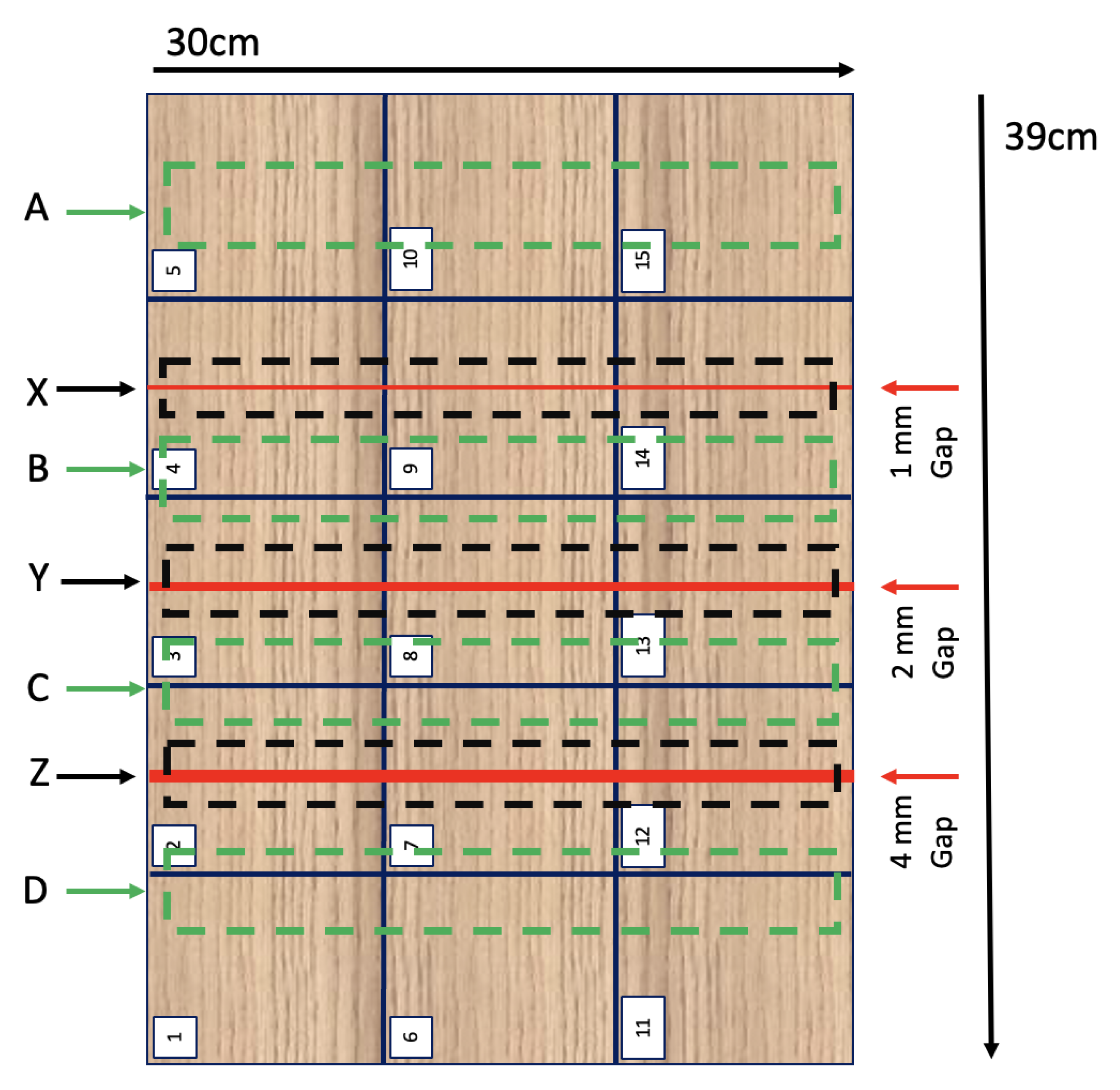
Section 3.1, using samples No.5 and No.6 to collect data pertaining to the air gap defect. Specifically, sample No.5 contains air gaps of 1 mm, 2 mm, and 4 mm for the first SC sample, and sample No.6 contains 6mm air gap. Figure 7 gives an illustration of the SC sample No.5 inner structure, our FMCW scanning took place where air gaps are present, i.e., areas labelled as A, B, C and D for healthy areas, as well as sections X, Y, and Z for areas containing the air voids defect. For the SC sample 6, we repeat our scanning process but instead scanned two areas/sections: healthy area, and areas with 6mm air gap.
After these scanning processes, we obtained sufficient RSA data to train our classification model with six classes as shown in Table 6. When given future RSA data from a selected WT blade area as input to this classification model, we can use the model output to identify whether the given data represent sub-surface defect, and the severity of such defects.
Raster scans were conducted at three distances: 5 cm, 10 cm and 15 cm from each target on the SC sample to ensure sufficient data for a richer training pool. Next, raster scans were conducted on using samples No.4 to collect data on interlaminar porosity/dry zone defect. Sample No.4 contains two dry zone areas. As depicted, the nature of these dry zone areas means that when conducting FMCW scanning, we can obtain RSA data representing three types of blade surface areas: areas with both the dry zone area itself and an adjacent healthy blade area; dry zone-only areas; healthy-only areas.
After these scanning processes, we obtained sufficient RSA data to train our classification model with three classes as shown in Table 7. When given future RSA data from a selected WT blade area as input to our classification model, we can use the model output to identify whether the given data represent the interlaminar porosity defect.
FMCW radar were placed at 5 cm, 10 cm, and 15 cm distances from the MC sample No.4 in Figure 6 for scanning, resulting in 179 scans for dry zone A and 177 scans for dry zone B.

5.3. Data Anaylsis and Results

We follow the same data analysis procedure as mentioned at Section 4.2 and Section 4.3, specifically, support Vector Machine, Bayesian Network, Decision Trees and Back Propagation network were implemented to explore the capability of machine learning approaches for this multi class classification problem. The classification model was trained using different forms of RSA data, e.g., the raw RSA data and processed data through different feature selection methods. The models were trained with 75% data from the raw data pool and tested with the remaining 25% data. The accuracy performance of different classifiers using different form of training data is shown at Table 8 and Table 9.

5.4. Discussion and Findings

Results in Table 8 and Table 9 illustrate the effectiveness of FMCW radar sensing and ML algorithm on detection of surface and subsurface defects, i.e., interlaminar porosity and air voids. From Table 8, we observe that the overall performance of all ML classifiers (SVM, Naive Bayes, Decision Tree and BP) achieved solid results for dry zone detection. When trained with full length of raw RSA data, SVM provided the best performance of 92.5% accuracy where as Naive Bayes has the least 70.8% accuracy rate. We also show that ML algorithms trained with compressed data also perform well, and in some cases even better than using the raw RSA data. When using full range of FD amplitude for training, our SVM classifier performance increased to 98.9% being the most accurate, while all other classifiers also saw improved performance from the Full length raw RSA signal case, with overall performance of over 82.8% accuracy rate for dry zone detection problems on WT blades. These results demonstrate that the frequency domain data transformed from FMCW RSA signals can be more revealing in terms of features and characteristics of composite materials defects.
In Table 9, we show results of using different classifiers to conduct WT blade diagnostics of air voids defect. We observe that the overall performance of different classifiers on air gap detection is relatively worse than those seen in dry-zone detection. For example, regardless of the type of data used for training, both SVM and Decision Tree algorithms saw reduction in accuracy. However, the evidence for whether Naive Bayes and BP are more accurate for air gap detection is mixed. Among all four classifiers, Decision Tree appears to be the least accurate for detecting air voids within WT blade inner structure.
Still, the highest level of classification performance were 94.1% where SVM is trained with full range of FD amplitude. When using selected range of FD amplitude, SVM achieved 93.9% accuracy. Comparably, Naive Bayes classifier also achieved satisfactory performance when trained with full (84.5%) and selected range (83.8%) FD amplitude. These two types of training data were obtained by feature selection of the raw RSA signals, and using these two types of data for training leads to better classification performance for all four algorithms compared to training with full length/compressed RSA data. This finding is also seen when examining WT blade surface defect of dry zones. In reality, FMCW might receive too much unnecessary RSA due to reflections from a more dynamic and complex environment, which will make the detection and analysis more challenging. Our results suggest that FMCW could potentially be a good candidate for flexible integrity evaluation for WTBs in practical applications with more careful and intelligent range selection and higher scan resolution from the radar.

6. Asset Integrity Dashboard

The Asset Integrity Dashboard(AID) was developed as an investigation into visualisation techniques for FMCW return signal data This work can be viewed online at https://smartsystems.hw.ac.uk/asset-integrity-dashboard-version-2/ (accessed on 29 January 2023). It was developed in Unity3D for Windows and HTML5 web integration. The data returned from the FMCW experiment is not immediately intuitive and requires analysis to understand. For operators with a lower working knowledge of FMCW technologies but have an understanding of subsurface defects and asset integrity, a more visual and intuitive method of displaying this data can be beneficial. The AID acts as a DT of a WTB section, with buttons on the left hand side allowing an operator to view different pieces of information about the asset, along with a 3D model of the WT blade section which changes appearance depending on what information is being displayed. An overview of the interface can be seen in Figure 8A.
Figure 8B shows the defect highlighted in the 3D model within the AID. A schematic of the sample with defect and a photograph of the sample with the defect highlighted are provided to assist identification of the defect.
The parts of information which can be displayed are:
  • Real Images of Sample—Photographs of the sample which is being twinned in the AID.
  • Sample Parameters—The supplied parameters of the sample (material composition, size, etc.).
  • Schematic of Sample—A pictorial schematic of the sample with defect area highlighted.
  • Experimental Setup—Photographs of the experimental setup of the FMCW with the sample.
  • Overlay of all graphs—Shows all return signal graphs.
  • Conclusion—A textual summary of the detected defect.
As a visual example, Figure 8C shows the “Overlay of All Graphs” display. This displays the return signal graph with colour coding where the colour coding on the graph matches up with the colour coding on the 3D model for improved reference. Additionally, there is improved interactivity as the user can click on each coloured row on the 3D model to view the RSA for each specific row.
The advantage of using an alternate display method such as this is it enables a more intuitive approach to viewing return signal data. This allows current operators to utilise FMCW technology without extensive retraining on data post-processing and interpretation. Future work in this area includes more visualisation techniques of the data (e.g., highlight critical parts of the return signal) and run-time generation of the graphs and model. Currently, all data shown are generated offline in MATLab and only screenshots are shown in the AID. Future work includes generating this information during runtime to enable for rapid remote asset integrity inspection.

7. Future Work and Discussion

Our future studies could focus on examining the resilience and sensitivity of FMCW radar to vibrations, varying weather and environmental conditions. In the current study, FMCW radar was mounted on a robotic arm for smooth scanning of the blade sample. However, in practice, WTBs often operate in harsh environments with strong winds, making smooth maneuvering of robotic arms difficult. Furthermore, future research could also explore the use of unmanned aerial vehicles (UAVs) for rapid inspection of WTBs located at significant heights, which would require the design of optimal UAV routes and positioning of the FMCW radar for efficient and accurate data capture under vibration. Additionally, this FMCW application could also be extended to identify the severity of defects on a WTB, different types of defects, and varying levels of defects throughout different stages of a WTB’s lifecycle. This would enable asset owners and managers to build a library of FMCW response data pertaining to varying WTB health status, which is currently lacking in literature. It is worth noting that our methodology highly depends on data availability and quality. However, collecting high-quality WTB data can be difficult and time-consuming. For example, it may be very diffuclt to collect high quality data on defects occurring at different stages of the entire WTB lifecycle.

8. Conclusions

The current methods for non-destructive evaluation (NDE) of wind turbine blades (WTBs) are highly labor-intensive and costly, and rely primarily on visual inspection. As the number of wind farms continues to increase, there is a pressing need to improve the consistency and accuracy of WTB evaluations, as well as to safely access both surface and subsurface characteristics. In response to this need, this paper presents a non-contact, low-power NDE approach that utilizes frequency-modulated continuous-wave (FMCW) radar analysis in conjunction with machine learning. The proposed method employs composite samples from the R&D division of EDF and a robotic arm for FMCW sensing. Results from classification models demonstrate that FMCW can accurately characterize composite material physical features, such as thickness, with 92.9% accuracy using a support vector machine (SVM) model and a full range of frequency domain amplitude for training. Furthermore, the method has the ability to distinguish variable surface defects, such as dry zones, with high accuracy of 98.9% (SVM) and 82.9% (Naive Bayes). Additionally, FMCW analysis is able to capture subsurface defects (air voids) of size 1mm with over 94.1% accuracy. In summary, this paper demonstrates the promising potential of FMCW in capturing WTB physical and defect information and the automation of this lightweight, compact, and low-power technology for advancing inspection procedures in NDE of composites. The paper also presents a digital twin of the WTB as an Asset Integrity Dashboard, which displays return signal data in an intuitive manner for those not familiar with the technology. Future research will focus on examining the resilience and sensitivity of FMCW radar to vibrations and environmental conditions, as well as the deployment of UAVs and FMCW for rapid inspection of WTBs.

Author Contributions

Conceptualization, D.F., W.T. and J.B.; methodology, W.T.; software, J.B., D.M. and S.H.; validation, W.T.; formal analysis, D.F. and J.B.; investigation, D.M.; resources, S.H.; data curation, W.T.; writing—original draft preparation, W.T.; writing—review and editing, D.F.; visualization, S.H.; supervision, D.F.; project administration, D.F.; funding acquisition, D.F. All authors have read and agreed to the published version of the manuscript.

Funding

This research was funded by the EPSRC Offshore Robotics for Certification of Assets Hub under Grant EP/R026173/1. The APC was funded by Heriot Watt University.

Acknowledgments

The experiments of this research were supported by MicroSense Technologies Ltd (MTL) in the provision of their patented microwave sensing technology (PCT/GB2017/053275), EDF R&D division in the provision of wind turbine composite samples.

Conflicts of Interest

The authors declare no conflict of interest.

References

  1. WWEA. Worldwide Wind Capacity Reaches 744 Gigawatts. Technical Report, World Wind Energy Association, 2021. Available online: https://wwindea.org/worldwide-wind-capacity-reaches-744-gigawatts (accessed on 29 January 2023).
  2. Barnes, M.; Brown, K.; Carmona, J.; Cevasco, D.; Collu, M.; Crabtree, C.; Crowther, W.; Djurovic, S.; Flynn, D.; Green, P.; et al. Technology Drivers in Windfarm Asset Management; Home Offshore: Singapore, 2018. [Google Scholar] [CrossRef]
  3. Kong, C.; Bang, J.; Sugiyama, Y. Structural investigation of composite wind turbine blade considering various load cases and fatigue life. Energy 2005, 30, 2101–2114. [Google Scholar] [CrossRef]
  4. Thomsen, O.T. Sandwich Materials for Wind Turbine Blades—Present and Future. J. Sandw. Struct. Mater. 2009, 11, 7–26. [Google Scholar] [CrossRef]
  5. Tucci, F.; Vedernikov, A. Design Criteria for Pultruded Structural Elements. In Encyclopedia of Materials: Composites; Brabazon, D., Ed.; Elsevier: Oxford, UK, 2021; pp. 51–68. [Google Scholar] [CrossRef]
  6. Yang, B.; Sun, D. Testing, inspecting and monitoring technologies for wind turbine blades: A survey. Renew. Sustain. Energy Rev. 2013, 22, 515–526. [Google Scholar] [CrossRef]
  7. Red, C. Wind turbine blades: Big and getting bigger. Compos. Technol. 2008. Available online: https://www.compositesworld.com/articles/wind-turbine-blades-big-and-getting-bigger (accessed on 29 January 2023).
  8. Raišutis, R.; Jasiuniene, E.; Sliteris, R.; Vladišauskas, A. The review of non-destructive testing techniques suitable for inspection of the wind turbine blades. Ultrasound 2008, 63, 26–30. [Google Scholar]
  9. Chou, J.S.; Chiu, C.K.; Huang, I.K.; Chi, K.N. Failure analysis of wind turbine blade under critical wind loads. Eng. Fail. Anal. 2013, 27, 99–118. [Google Scholar] [CrossRef]
  10. Liu, W.; Tang, B.; Han, J.; Lu, X.; Hu, N.; He, Z. The structure healthy condition monitoring and fault diagnosis methods in wind turbines: A review. Renew. Sustain. Energy Rev. 2015, 44, 466–472. [Google Scholar] [CrossRef]
  11. Li, D.; Ho, S.C.M.; Song, G.; Ren, L.; Li, H. A review of damage detection methods for wind turbine blades. Smart Mater. Struct. 2015, 24, 033001. [Google Scholar] [CrossRef]
  12. Besnard, F.; Bertling, L. An Approach for Condition-Based Maintenance Optimization Applied to Wind Turbine Blades. IEEE Trans. Sustain. Energy 2010, 1, 77–83. [Google Scholar] [CrossRef]
  13. Yang, R.; He, Y.; Zhang, H. Progress and trends in nondestructive testing and evaluation for wind turbine composite blade. Renew. Sustain. Energy Rev. 2016, 60, 1225–1250. [Google Scholar] [CrossRef]
  14. Sutherland, H.; Beattie, A.; Hansche, B.; Musial, W.; Allread, J.; Johnson, J.; Summers, M. The Application of Non-Destructive Techniques to the Testing of a Wind Turbine Blade; Sandia National Labs.: Albuquerque, NM, USA, 1994. [Google Scholar] [CrossRef]
  15. García Márquez, F.P.; Peco Chacón, A.M. A review of non-destructive testing on wind turbines blades. Renew. Energy 2020, 161, 998–1010. [Google Scholar] [CrossRef]
  16. Kim, D.Y.; Kim, H.B.; Jung, W.S.; Lim, S.; Hwang, J.H.; Park, C.W. Visual testing system for the damaged area detection of wind power plant blade. In Proceedings of the IEEE ISR, Seoul, Republic of Korea, 24–26 October 2013; pp. 1–5. [Google Scholar] [CrossRef]
  17. Wallace, J.; Dawson, M. O&M strategies: Wind turbine blades. Renew. Energy Focus 2009, 10, 36–41. [Google Scholar] [CrossRef]
  18. Raišutis, R.; Tiwari, K.A.; Žukauskas, E.; Tumšys, O.; Draudvilienė, L. A Novel Defect Estimation Approach in Wind Turbine Blades Based on Phase Velocity Variation of Ultrasonic Guided Waves. Sensors 2021, 21, 4879. [Google Scholar] [CrossRef] [PubMed]
  19. Jasiuniene, E.; Raišutis, R.; literis, R.; Voleiis, A.; Vladiauskas, A.; Mitchard, D.; Amos, M. NDT of wind turbine blades using adapted ultrasonic and radiographic techniques. Insight—Non-Destr. Test. Cond. Monit. 2009, 51, 477–483. [Google Scholar] [CrossRef]
  20. Schroeder, K.; Ecke, W.; Apitz, J.; Lembke, E.; Lenschow, G. A fibre Bragg grating sensor system monitors operational load in a wind turbine rotor blade. Meas. Sci. Technol. 2006, 17, 1167–1172. [Google Scholar] [CrossRef]
  21. Hernandez Crespo, B. Damage Sensing in Blades. In MARE-WINT: New Materials and Reliability in Offshore Wind Turbine Technology; Ostachowicz, W., McGugan, M., Schröder-Hinrichs, J.U., Luczak, M., Eds.; Springer International Publishing: Cham, Switzerland, 2016; pp. 25–52. [Google Scholar] [CrossRef]
  22. Du, Y.; Zhou, S.; Jing, X.; Peng, Y.; Wu, H.; Kwok, N. Damage detection techniques for wind turbine blades: A review. Mech. Syst. Signal Process. 2020, 141, 106445. [Google Scholar] [CrossRef]
  23. Mishnaevsky, L.; Branner, K.; Petersen, H.N.; Beauson, J.; McGugan, M.; Sørensen, B.F. Materials for Wind Turbine Blades: An Overview. Materials 2017, 10, 1285. [Google Scholar] [CrossRef] [Green Version]
  24. Gupta, R.; Huo, D.; White, M.; Jha, V.; Stenning, G.B.; Pancholi, K. Novel method of healing the fibre reinforced thermoplastic composite: A potential model for offshore applications. Compos. Commun. 2019, 16, 67–78. [Google Scholar] [CrossRef]
  25. Mandell, J.; Samborsky, D. Composite materials fatigue issues in wind turbine blade construction. Int. SAMPE Symp. Exhib. (Proc.) 2008. Available online: https://citeseerx.ist.psu.edu/document?repid=rep1&type=pdf&doi=80c5f68e0501d6cf56a6502f099607ec4a6e3acc (accessed on 29 January 2023).
  26. Saeedifar, M.; Ahmadi Najafabadi, M.; Yousefi, J.; Mohammadi, R.; Hosseini Toudeshky, H.; Minak, G. Delamination analysis in composite laminates by means of Acoustic Emission and bi-linear/tri-linear Cohesive Zone Modeling. Compos. Struct. 2017, 161, 505–512. [Google Scholar] [CrossRef]
  27. Liu, P.; Xu, D.; Li, J.; Chen, Z.; Wang, S.; Leng, J.; Zhu, R.; Jiao, L.; Liu, W.; Li, Z. Damage mode identification of composite wind turbine blade under accelerated fatigue loads using acoustic emission and machine learning. Struct. Health Monit. 2020, 19, 1092–1103. [Google Scholar] [CrossRef]
  28. Liu, Z.; Wang, X.; Zhang, L. Fault Diagnosis of Industrial Wind Turbine Blade Bearing Using Acoustic Emission Analysis. IEEE Trans. Instrum. Meas. 2020, 69, 6630–6639. [Google Scholar] [CrossRef]
  29. Gholizadeh, S. A review of non-destructive testing methods of composite materials. Procedia Struct. Integr. 2016, 1, 50–57. [Google Scholar] [CrossRef]
  30. Grosse, C. Acoustic emission (AE) evaluation of reinforced concrete structures. In Non-Destructive Evaluation of Reinforced Concrete Structures; Woodhead Publishing Series in Civil and Structural Engineering; Maierhofer, C., Reinhardt, H.W., Dobmann, G., Eds.; Woodhead Publishing: Sawston, UK, 2010; Volume 2, pp. 185–214. [Google Scholar] [CrossRef]
  31. Soerensen, B.F.; Lading, L.; Sendrup, P. Fundamentals for Remote Structural Health Monitoring of Wind Turbine Blades—A Pre-Project; Materials Research Dept., Risoe National Lab.: Roskilde, Denmark, 2002. [Google Scholar]
  32. Lu, Y. Non-Destructive Evaluation on Concrete Materials and Structures Using Cement-Based Piezoelectric Sensor; Hong Kong University of Science and Technology: Hong Kong, China, 2010. [Google Scholar]
  33. Raišutis, R.; Kažys, R.; Mažeika, L. Application of the ultrasonic pulse-echo technique for quality control of the multi-layered plastic materials. NDT E Int. 2008, 41, 300–311. [Google Scholar] [CrossRef]
  34. Amenabar, I.; Mendikute, A.; López-Arraiza, A.; Lizaranzu, M.; Aurrekoetxea, J. Comparison and analysis of non-destructive testing techniques suitable for delamination inspection in wind turbine blades. Compos. Part B Eng. 2011, 42, 1298–1305. [Google Scholar] [CrossRef]
  35. Mook, G.; Lange, R.; Koeser, O. Non-destructive characterisation of carbon-fibre-reinforced plastics by means of eddy-currents. Compos. Sci. Technol. 2001, 61, 865–873. [Google Scholar] [CrossRef]
  36. Pieraccini, M.; Parrini, F.; Fratini, M.; Atzeni, C.; Spinelli, P. In-service testing of wind turbine towers using a microwave sensor. Renew. Energy 2008, 33, 13–21. [Google Scholar] [CrossRef]
  37. Jeong, H.; Hsu, D.K.; Liaw, P.K. Anisotropic conductivities of multiphase particulate metal-matrix composites. Compos. Sci. Technol. 1998, 58, 65–76. [Google Scholar] [CrossRef]
  38. Moll, J. Numerical and Experimental Analysis of Defect Detection in Jointed Electromagnetic Waveguides. In Proceedings of the 2019 13th European Conference on Antennas and Propagation (EuCAP), Krakow, Poland, 31 March–5 April 2019; pp. 1–4. [Google Scholar]
  39. Heuer, H.; Schulze, M.; Pooch, M.; Gäbler, S.; Nocke, A.; Bardl, G.; Cherif, C.; Klein, M.; Kupke, R.; Vetter, R.; et al. Review on quality assurance along the CFRP value chain – Non-destructive testing of fabrics, preforms and CFRP by HF radio wave techniques. Compos. Part B Eng. 2015, 77, 494–501. [Google Scholar] [CrossRef]
  40. Li, Z.; Haigh, A.; Soutis, C.; Gibson, A.; Wang, P. A review of microwave testing of glass fibre-reinforced polymer composites. Nondestruct. Test. Eval. 2019, 34, 429–458. [Google Scholar] [CrossRef]
  41. Kharkovsky, S.; Zoughi, R. Microwave and millimeter wave nondestructive testing and evaluation - Overview and recent advances. IEEE Instrum. Meas. Mag. 2007, 10, 26–38. [Google Scholar] [CrossRef]
  42. Park, B.; Sohn, H.; Yeum, C.M.; Truong, T.C. Laser ultrasonic imaging and damage detection for a rotating structure. Struct. Health Monit. 2013, 12, 494–506. [Google Scholar] [CrossRef]
  43. Zhang, H.; Jackman, J. Feasibility of Automatic Detection of Surface Cracks in Wind Turbine Blades. Wind Eng. 2014, 38, 575–586. [Google Scholar] [CrossRef]
  44. Katnam, K.B.; Comer, A.J.; Roy, D.; da Silva, L.F.M.; Young, T.M. Composite Repair in Wind Turbine Blades: An Overview. J. Adhes. 2015, 91, 113–139. [Google Scholar] [CrossRef]
  45. Cheng, L.; Tian, G.Y. Comparison of Nondestructive Testing Methods on Detection of Delaminations in Composites. J. Sens. 2012, 2012, 408437. [Google Scholar] [CrossRef]
  46. Marsh, G. Meeting the challenge of wind turbine blade repair. Reinf. Plast. 2011, 55, 32–36. [Google Scholar] [CrossRef]
  47. Khadka, A.; Fick, B.; Afshar, A.; Tavakoli, M.; Baqersad, J. Non-contact vibration monitoring of rotating wind turbines using a semi-autonomous UAV. Mech. Syst. Signal Process. 2020, 138, 106446. [Google Scholar] [CrossRef]
  48. Desmulliez, M.; Pavuluri, S.K.; Flynn, D.; Herd, D. Microwave Cavity Sensor. U.S. Patent 10024806B2, 7 November 2013. Available online: https://patents.google.com/patent/WO2013164627A1/en (accessed on 29 January 2023).
  49. Blanche, J.; Flynn, D.; Lewis, H.; Couples, G.; Cheung, R. Analysis of geomaterials using frequency modulated continuous wave radar in the X-band. In Proceedings of the 2017 IEEE 26th International Symposium on Industrial Electronics (ISIE), Edinburgh, UK, 19–21 June 2017; pp. 1376–1381. [Google Scholar] [CrossRef]
  50. Tang, W.; Mitchell, D.; Blanche, J.; Gupta, R.; Flynn, D. Machine Learning Analysis of Non-Destructive Evaluation Data from Radar Inspection of Wind Turbine Blades. In Proceedings of the 2021 IEEE International Conference on Sensing, Diagnostics, Prognostics, and Control (SDPC), Weihai, China, 13–15 August 2021; pp. 122–128. [Google Scholar] [CrossRef]
  51. Blanche, J.; Mitchell, D.; Gupta, R.; Tang, A.; Flynn, D. Asset Integrity Monitoring of Wind Turbine Blades with Non-Destructive Radar Sensing. In Proceedings of the 2020 11th IEEE Annual Information Technology, Electronics and Mobile Communication Conference (IEMCON), Vancouver, BC, Canada, 4–7 November 2020; pp. 498–504. [Google Scholar] [CrossRef]
  52. Blanche, J.; Buckman, J.; Lewis, H.; Flynn, D.; Couples, G. Frequency Modulated Continuous Wave Analysis of Dynamic Load Deformation in Geomaterials. In Proceedings of the Offshore Technology Conference, Houston, TX, USA, 4–7 May 2020. [Google Scholar] [CrossRef]
  53. Herd, D. Microwave Based Monitoring System for Corrosion under Insulation. Ph.D. Thesis, Heriot-Watt University, School of Engineering and Physical Sciences, Edinburgh, UK, 2016. [Google Scholar]
  54. Blanche, J.; Lewis, H.; Couples, G.D.; Buckman, J.; Lenoir, N.; Tengattini, A.; Flynn, D. Dynamic Fluid Ingress Detection in Geomaterials Using K-Band Frequency Modulated Continuous Wave Radar. IEEE Access 2020, 8, 111027–111041. [Google Scholar] [CrossRef]
  55. Blanche, J.; Flynn, D.; Lewis, H.; Couples, G.D.; Buckman, J.; Bailey, C.; Tilford, T. Analysis of Sandstone Pore Space Fluid Saturation and Mineralogy Variation via Application of Monostatic K-Band Frequency Modulated Continuous Wave Radar. IEEE Access 2018, 6, 44376–44389. [Google Scholar] [CrossRef]
  56. Zaki, O.; Flynn, D.; Blanche, J.; Roe, J.; Kong, L.; Mitchell, D.; Lim, T.; Harper, S.; Robu, V. Self-Certification and Safety Compliance for Robotics Platforms. In Proceedings of the Offshore Technology Conference, Houston, TX, USA, 4–7 May 2020. [Google Scholar] [CrossRef]
  57. Mitchell, D.; Blanche, J.; Zaki, O.; Roe, J.; Kong, L.; Harper, S.; Robu, V.; Lim, T.; Flynn, D. Symbiotic System of Systems Design for Safe and Resilient Autonomous Robotics in Offshore Wind Farms. IEEE Access 2021, 9, 141421–141452. [Google Scholar] [CrossRef]
  58. Mitchell, D.; Blanche, J.; Harper, S.; Lim, T.; Gupta, R.; Zaki, O.; Tang, W.; Robu, V.; Watson, S.; Flynn, D. A review: Challenges and opportunities for artificial intelligence and robotics in the offshore wind sector. Energy AI 2022, 8, 100146. [Google Scholar] [CrossRef]
  59. Gupta, R.; Mitchell, D.; Blanche, J.; Harper, S.; Tang, W.; Pancholi, K.; Baines, L.; Bucknall, D.G.; Flynn, D. A Review of Sensing Technologies for Non-Destructive Evaluation of Structural Composite Materials. J. Compos. Sci. 2021, 5(12), 319. [Google Scholar] [CrossRef]
  60. Mitchell, D.; Blanche, J.; Flynn, D. An Evaluation of Millimeter-wave Radar Sensing for Civil Infrastructure. In Proceedings of the 2020 11th IEEE Annual Information Technology, Electronics and Mobile Communication Conference (IEMCON), Vancouver, BC, Canada, 4–7 November 2020; pp. 216–222. [Google Scholar] [CrossRef]
  61. Hill, R.M. Dielectric Properties and Materials. In Electronic Materials; Miller, L.S., Mullin, J.B., Eds.; Springer: Boston, MA, USA, 1991. [Google Scholar]
  62. Jureczko, M.; Pawlak, M.; Mężyk, A. Optimisation of wind turbine blades. J. Mater. Process. Technol. 2005, 167, 463–471. [Google Scholar] [CrossRef]
  63. Griffin, D.A.; Ashwill, T.D. Blade System Design Studies Volume I: Composite Technologies for Large Wind Turbine Blades. In Composite Technologies for Large Wind Turbine Blades; Sandia National Lab. (SNL-NM): Albuquerque, NM, USA; Sandia National Lab. (SNL-CA): Livermore, CA, USA, 2002. [Google Scholar]
  64. ltd, U.R. UR3e Robot. Available online: https://www.universal-robots.com/products/ur3-robot/ (accessed on 29 January 2023).
  65. Kecman, V. Support Vector Machines—An Introduction. In Support Vector Machines: Theory and Applications; Wang, L., Ed.; Springer: Berlin/Heidelberg, Germany, 2005; pp. 1–47. [Google Scholar] [CrossRef]
  66. Friedman, N.; Geiger, D.; Goldszmidt, M. Bayesian network classifiers. Mach. Learn. 1997, 29, 131–163. [Google Scholar] [CrossRef]
  67. Buscema, M. Back propagation neural networks. Subst. Use Misuse 1998, 33, 233–270. [Google Scholar] [CrossRef] [PubMed]
  68. Rokach, L.; Maimon, O. Data Mining with Decision Trees, 2nd ed.; World Scientific: Singapore, 2014. [Google Scholar] [CrossRef]
  69. Jolliffe, I.T. Principal Component Analysis; Springer: Berlin/Heidelberg, Germany, 2002. [Google Scholar]
Figure 1. Block diagram of the sensor setup and analytical workflow, where the red (clockwise) arrows indicate the transmitted signal stages and the blue (counter-clockwise) arrows represent the received signal and data processing stages.
Jcs 07 00075 g001
Figure 2. FMCW Radar setup for procedures outlined.
Jcs 07 00075 g002
Figure 3. (top left) Composite material test sample No.1 with monolithic thickness of 48.7 mm, (top right) No.2 with monolithic thickness of 51.2 mm, (bottom left) No.3 with sandwich composites with thickness of 27.8 mm, (bottom right) Raster scanning on test samples using UR3 robot manipulator arm.
Jcs 07 00075 g003
Figure 4. Machine learning classification modelling workflow.
Jcs 07 00075 g004
Figure 5. Confusion matrix of model performance.
Jcs 07 00075 g005
Figure 6. Illustration of defects within samples (left: interlaminar porosity, right: air voids in balsa).
Jcs 07 00075 g006
Figure 7. Data collection of defect and healthy area of samples No.5, areas labelled as A, B, C and D represent for healthy areas, where areas X, Y, and Z represent for areas containing the air voids defect of different sizes.
Jcs 07 00075 g007
Figure 8. (A). Overview of AID interface. Buttons on the left allow specific information to be overlaid, with a 3D model of the asset in the middle. (B). Visualisation of the sample defect in the AID. The defect is highlighted in red. (C). Visualisation of all return signal graphs in the AID. Row colours in the graph match up to the WT 3D object.
Jcs 07 00075 g008
Table 1. Summary of NDE methods on WTBs with their advantages and limitations.
Method of NDE RefsAdvantageDisadvantageCritical Analysis
Visual inspection [13,16,24]Low cost; Simple to carry outLimited to surface defects; Inspector safety concerns; Depends on camera quality and inspector skills; Time consuming; Affected by weather conditionsUsed for large structures (e.g., bridges, WTBs) visible surface defect inspections from a safe distance, can be combined with UAV.
Acoustic Emissions [11,15,26,27,28]High Resolution Triangulate; Can be used on in-service assets; Good accuracy in short distance; Passive NDT techniqueContact-based, requires sensors to be embedded; Sensitive to noise disturbance; Vibrations affect resultsUsed for static sensing with easy access; Suitable for glass fibre reinforced plastic materials
Ultrasonic [13,33,34,42]Low computation cost; Good accuracy; May be used for large-are, in-serviceContact-based, requires couplant, Sound attenuation, Scanner required, May need expensive hardwareCan detect early stage faults and fault locations, such as ice thickness and delamination
Strain measurement [20,31]Integrated within bladesDifficult to retrofitCan monitor operational loads
Optical [43,44]Non-contact, high sensitivitySensitive to small thickness, expensiveConduct surface inspection for large areas in short time
Electromagnetic [13,26,35,36,37,38,39,40,41,45]Non-contact and Low costScanner is required, Sensitive to alignment orientationSuitable for delamination detection of composite material such as CFRP
Table 2. FMCW parameters used during the investigation.
ParameterValue
Frequency BandK Band (24–25.5 GHz)
Chirp Duration300 ms
Bandwidth1.5 GHz
Data Acquisition Frequency1 Hz
Table 3. Performance of different ML models with TD dataset.
AlgorithmFull Length of RSA SignalCompressed Length of Raw RSA Signal
SVM95%91%
Naïve Bayes80.7%76.1%
Decision Tree87.7%75.6%
BP81.7%78.7%
Table 4. Performance of different ML models with FD dataset.
AlgorithmFull Range of FD AmplitudeSelected Range of FD Amplitude
SVM98.5%92.9%
Naïve Bayes84.8%82.8%
Decision Tree88.9%88.6%
BP84.5%79.3%
Table 5. Detailed specification of samples with defects.
SampleDefect TypeDefect SizeSample Size
No.4Interlaminar porosityleft: 12 cm × 9 cm;360 mm × 385 mm × 51.4 mm
(Dry zone)right: 13 cm × 11 cm
No.5Air voids in balsa1 mm, 2 mm, 4 mm355 mm × 390 mm × 27.8 mm
No.6Air voids in balsa6 mm300 mm × 390 × 28 mm
Table 6. Characterization classes for air voids defect.
ClassesSurface/Subsurface CharacterizationSample No.
1surface area contains 1mm air voids in balsaNo.5
2surface area contains 2mm air voids in balsaNo.5
3surface area contains 4mm air voids in balsaNo.5
4surface area contains 6mm air voids in balsaNo.6
5healthy surface areaNo.5
6healthy surface areaNo.6
Table 7. Characterization classes for Interlaminar porosity defect.
ClassesSurface/Subsurface CharacterizationSample No.
1Healthy areaNo.4
2Defective areaNo.4
3Healthy and defective joint areaNo.4
Table 8. Accuracy performance of different classifiers of interlaminar porosity defect using different source of training data.
ClassifierFull Length of Raw RSA SignalCompressed Length of Raw RSA SignalFull Range of FD AmplitudeSelected Range of FD Amplitude
SVM92.5%90.9%98.9%96.9%
Naïve Bayes70.8%68.8%82.9%80.9%
Decision Tree84.9%79.6%90.9%86.9%
BP80.9%78.6%83.9%87.9%
Table 9. Accuracy performance of different classifiers of air voids defect using different source of training data.
AlgorithmFull Length of RSA SignalCompressed Length of RSA SignalFull Range of FD AmplitudeSelected Range of FD Amplitude
SVM79.2%75.9%94.1%93.9%
Naïve Bayes80.3%77.8%84.5%83.8%
Decision Tree71.9%69.6%70.1%68.1%
BP80.1%78.6%88.3%82.7%
Disclaimer/Publisher’s Note: The statements, opinions and data contained in all publications are solely those of the individual author(s) and contributor(s) and not of MDPI and/or the editor(s). MDPI and/or the editor(s) disclaim responsibility for any injury to people or property resulting from any ideas, methods, instructions or products referred to in the content.

