Article

Areal Analysis Investigation of Selective Laser Melting Parts

Department of Mechanical and Aerospace Engineering, Sapienza University of Rome, 00184 Rome, Italy
*
Author to whom correspondence should be addressed.
J. Manuf. Mater. Process. 2022, 6(4), 83; https://doi.org/10.3390/jmmp6040083
Submission received: 16 July 2022 / Revised: 1 August 2022 / Accepted: 1 August 2022 / Published: 4 August 2022
(This article belongs to the Special Issue Laser-Based Manufacturing II)

Abstract

:
Selective laser melting is an additive manufacturing technology used to fabricate metal parts characterized by complex geometries that are difficult or impossible to produce with conventional production methods. One of the major drawbacks of laser melting is the poor surface quality that typically is not satisfactory for functional applications. The aim of this work is to use areal analysis to characterize selective laser melting surfaces. The results highlight a marked variability and anisotropy that cannot be evaluated through traditional measurement. The building orientation and secondary finishing operations are analyzed and discussed. Findings demonstrate how areal analysis can be used to determine how to implement barrel finishing with the aim of reducing anisotropy and increasing surface quality.

1. Introduction

Additive manufacturing (AM) is a set of relatively new technologies that helps manufacturers to produce physical parts directly from a computer model by adding layers of material on top of each other. These technologies have proven to be useful when producing complex, expensive, and time-consuming parts. In such cases, the entire process produces less waste than traditional methods, both environmentally and economically. AM is adopted by many industries, i.e., automotive, aerospace, biomedical, and many others, because of the wide range of materials and machines available [1].
The AM process studied in this work is selective laser melting (SLM), which belongs to the powder bed fusion category [2]. SLM is one of the fastest-growing technologies, as it enables the production of metal shapes that are difficult or impossible to obtain with conventional production methods [3,4].
Besides providing numerous advantages, there are also some serious limitations when using SLM. The involvement of various processing parameters and their influence on the resulting surfaces determine the attainable quality of the fabricated parts to be insufficient for functional applications in most cases [5,6,7,8,9].
Because the resulting surface quality can considerably influence the properties of the final product, it is vital to understand the causes of surface imperfections to improve the quality of final products [10].
SLM surface quality is affected by various causes, e.g., the formation of microstructures and defects, such as pores, slags, cracks, incomplete fusion holes, and other surface anomalies [11,12,13].
The microstructures formed by SLM differ from those of conventional production methods [14,15]. These variations depend upon several factors, such as the processing parameters [9,16], the surface tension, solidification rates, and whether the fusion is well-controlled during fabrication [17].
The tuning and control of process parameters are important with respect to obtaining the desired geometries, mechanical properties, microstructures, and surface quality. Volumetric energy density (VED), i.e., the laser beam energy transmitted to a volumetric unit of powder material, is a critical manufacturing factor to consider because it is correlated with several exposure and scanning parameters [18]. The VED directly impacts the shape, size, temperature, and cooling rates within and near the melt pool and could cause residual stresses with a consequent distortion of the fabricated part [19]. Moreover, it was demonstrated that modifications of the VED during the SLM process determine variations in the surface quality and microstructure of the part [20].
Furthermore, the obtainable surface roughness is affected by other specific problems. In [21], the authors distinguished between balling phenomenon and satellite formation. The former is defined as the formation of large spheres of molten and solidified material partially incorporated into the processed layer. Conversely, the latter is defined as particles sticking to the surface due to the melt spattering or partial remelting with insufficient energy to incorporate them into the melt pool. With respect to the final roughness, balling is the most effective phenomenon, as it is characterized by dimensions larger than the laser spot diameter.
Additionally, the surface roughness and morphology are affected by the staircase effect, which is directly related to the building orientation, the layer thickness, and the designed geometry [22].
The surface quality of SLM is a crucial aspect to consider for the fabrication of functional and aesthetic components. Typically, other post-processing operations must be performed to enhance the surface quality of selective laser-melted (SLMed) parts, such as shoot peening [23,24], sandblasting [25], machining [26,27], and barrel finishing (BF) [28,29]. Such operations improve the surface in terms of roughness; measurement of the surface state during these processes is necessary to evaluate the evolution of the surface morphology and to understand when to stop the finishing process. Surface monitoring is important, especially for post-processing processes such as BF, which are difficult to predict because of the lack of models and formulations.
The importance of obtaining sufficient surface quality increases the need to measure the overall surface topography during manufacturing operations. For more than a century, 2D profile measurements were adequate to control industrial surface fabrication. With the increasing need to control a wide range of functionalities (optical, tribological, fluidic, biological, etc.), a considerable growth in the use of areal measurements has occurred. Many standards have been introduced, as well as parameters and characterization methods able to provide specific information in a broad range of subject areas [30].
Some of the new parameters are extensions of the well-established roughness parameters. Norms such as ISO 4278 [31] for parameter definition and ISO 4288 [32] for selection of the cutoffs have been regularly confirmed without modifications. A milestone in areal analysis is the recent ISO 25178 [33], which establishes a new basis for surface texture characterization. It divides the areal parameters into several categories, such as height, functional, volume, and spatial parameters, etc.
Height parameters, such as Sa (arithmetical absolute mean of the referred heights of the surface) and Sq (root mean square of referred heights) are evaluated over the complete 3D surface to indicate significant deviations in the texture characteristics. Other height parameters, such as Sp, Sv, and Sz, are calculated from the surface’s maximum peak and minimum valley height. The shape of the height distribution is given by Ssk and Sku for symmetry and sharpness, respectively. A negative Ssk value indicates that the surface is made up of a predominant plateau and deep valleys, whereas a positive value is related to a surface with a disproportionate number of peaks. A Gaussian surface has a symmetrical shape; thus, the Ssk is zero. The Sku, in this case, is 3 whereas a surface with a well spread-out distribution is platykurtic (Sku < 0), i.e., it is possible to identify a plateau-honed surface with relatively flat peaks and deep valleys. Conversely, an Sku > 0 indicates that the surface is composed of many high peaks and low valleys (leptokurtic distribution).
Functional parameters are calculated based on the material ratio curve (the Abbott-Firestone curve). Two material volumes (Vmp and Vmc) and two void volume parameters (Vvc and Vvv) are defined. Vmp indicates the amount of material that is prone to be worn away at a specific material ratio, whereas the core material volume (Vmc) is related to the amount of remaining material that is capable of load supporting after the removal of levels of the surface. Vvc and Vvv are useful for coating applications, as well as when fluid flow is considered.
Spatial parameters are indicators of uniformity of the surface, and their calculation is derived from the autocorrelation function (ACF). Str is defined as the minimum to maximum radii ratio calculated by thresholding the central ACF peak. If the surface shows a privileged orientation, the radii are markedly different, resulting in a low Str value. Conversely, isotropic surfaces have an approximatively circular central peak, and the Str tends toward a value of 1. The minimum radius value is defined by the Sal parameter, which provides a useful indication of the spectral content of the surface. Determination of privileged directions of the surface texture is possible through the Fourier spectrum. A widely used diagram is the so-called spectrum polar graph, which plots the power spectrum in each direction; the highest values correspond to the most important texture direction.
Another important surface feature is flatness. Definitions of the elements necessary for proper determination of the flatness deviation (such as the nominal, reference, and real planes) are provided in ISO 1011 [34]. A commonly used parameter is the FLTq, which is defined as the square root of the sum of the squares of the local deviation from the reference plane [35].
In this work, we employ areal analysis to study surface textures in two motivating case studies.
Our aim is to highlight how areal analysis can identify important surface features in SLM parts and suggest reasonable causal sources. We investigate the effect of building orientation and BF post-processing surface evolution on simple geometries. Traditional 2D profile measurements are applied for comparison, demonstrating a marked variability and anisotropy of SLMed surfaces.
The analysis is extended to a complex geometry in the second case study to demonstrate BF accessibility issues. The evaluation of specific outcomes allows for understanding of how the secondary finishing operation must be implemented. A typical critical point is the selection of the processing time, which typically must assure the best attainable surface quality. This knowledge informs when to stop the operation to avoid further modifications that could damage the outcome and nullify the previous technological steps.

2. Material and Methods

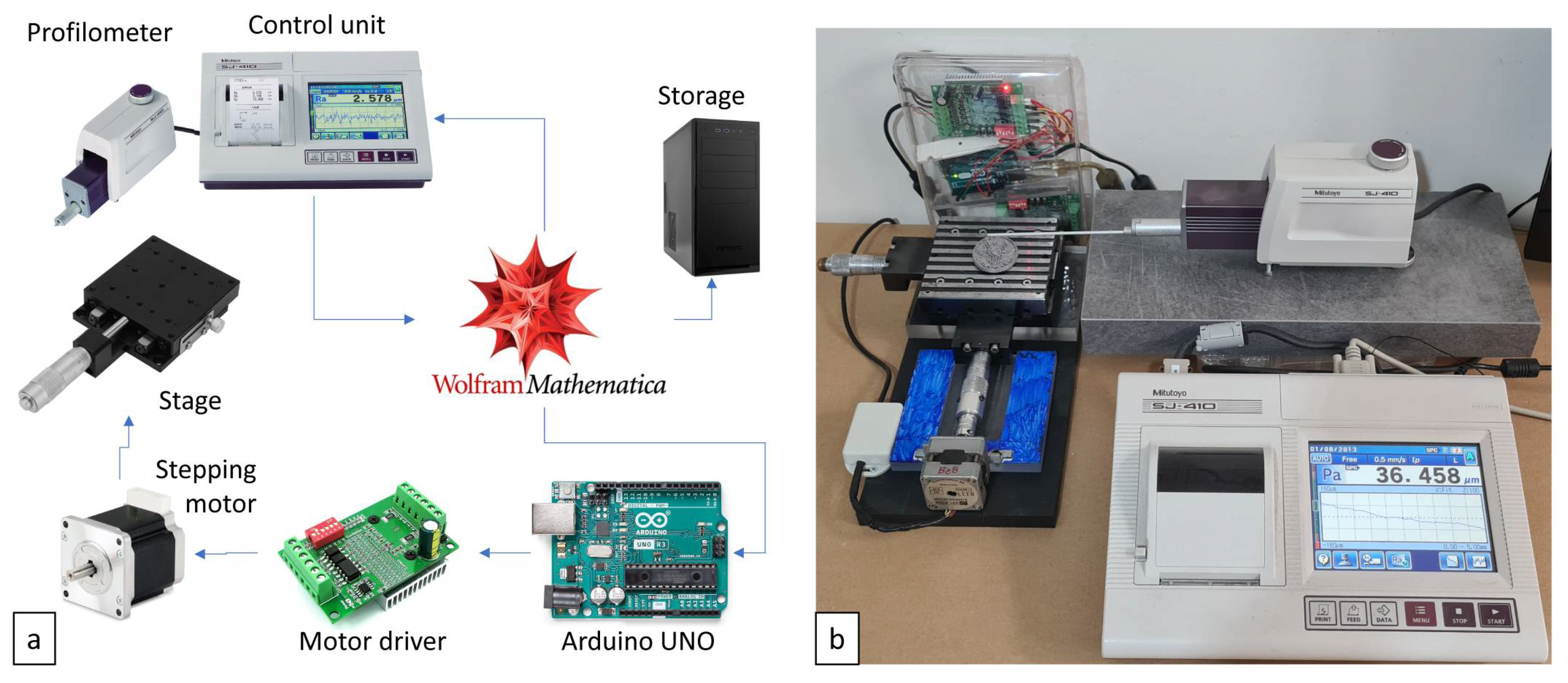
2.1. 3D-Map Measurement

The approach used in this work is based on the use of maps extracted from different surfaces. As our focus is on areal analysis of SLM surfaces, which are naturally affected by a high degree of vertical deviation (high roughness and large Sz), there is a need to perform high-resolution measurements on these surfaces. The most reliable method is measurement with roughness profilometer.
The system chosen for the mentioned purpose is Mitutoyo SJ 410 (Mitutoyo, Sakado, Japan), which is typically used for roughness measurement. A stylus with a 180 mm length and a 2µm tip radius is used, resulting in a maximum vertical height of 2400 µm. This feature is useful for long measures on curved components. The vertical precision is 16 nm, which is sufficient for SLM profiles. The measurement is reliable as long as the contact does not cause local surface deformation. Therefore, the pre-amplifier is balanced so that the contact force is 0.75 mN, which causes negligible stress-induced deformation on metallic parts, e.g., an aluminum or titanium alloy. The high traveling distance allows for exploration of large areas. The main information from the profilometer datasheet is summarized in Table 1.
Map data were acquired without applying filtering. For comparison, some single profiles were filtered according to ISO 16610 [36], and roughness parameters were calculated according to ISO 4287 [31].
3D maps are achieved by repeating the profile measurements transversely. The positioning is assured by a stage moved by a stepping motor and commanded by dedicated electronics.
In order to assure adequate sequencing of the operations and ensure appropriate positioning dynamics, the stage and the profilometer are commanded in a unique platform. Wolfram Mathematica 13.1 (Wolfram Research, Inc., Champaign, IL, USA) is used both for commanding/controlling and data analysis. The system framework is shown in Figure 1a. A Mitutoyo-specific language is adopted to fully sense the profilometer through a dedicated control unit. Arduino UNO (Arduino, Somerville, MA, USA) is selected because it provides low-level, general-purpose input and output through serial dialoguing with Wolfram Language.
The developed code has the goal of fully automatizing the measurements according to the following operations:
  • The stylus is positioned at the beginning of the measurement area;
  • The profilometer starts measurement at 0.5 mm/s speed;
  • The profile is cropped at the beginning and the end to eliminate starting and stopping dynamics;
  • The data are acquired as an x-z temporary file;
  • The stylus returns to its initial position at a 2 mm/s speed;
  • The stage moves the part to the next y position;
  • The operation pauses for 1 s to avoid vibration phenomena;
  • Operation 2 is repeated until the y positioning is complete; and
  • The map is built by composing all the temporary files in an x-y-z structure.
The layout of the system is shown in Figure 1b.

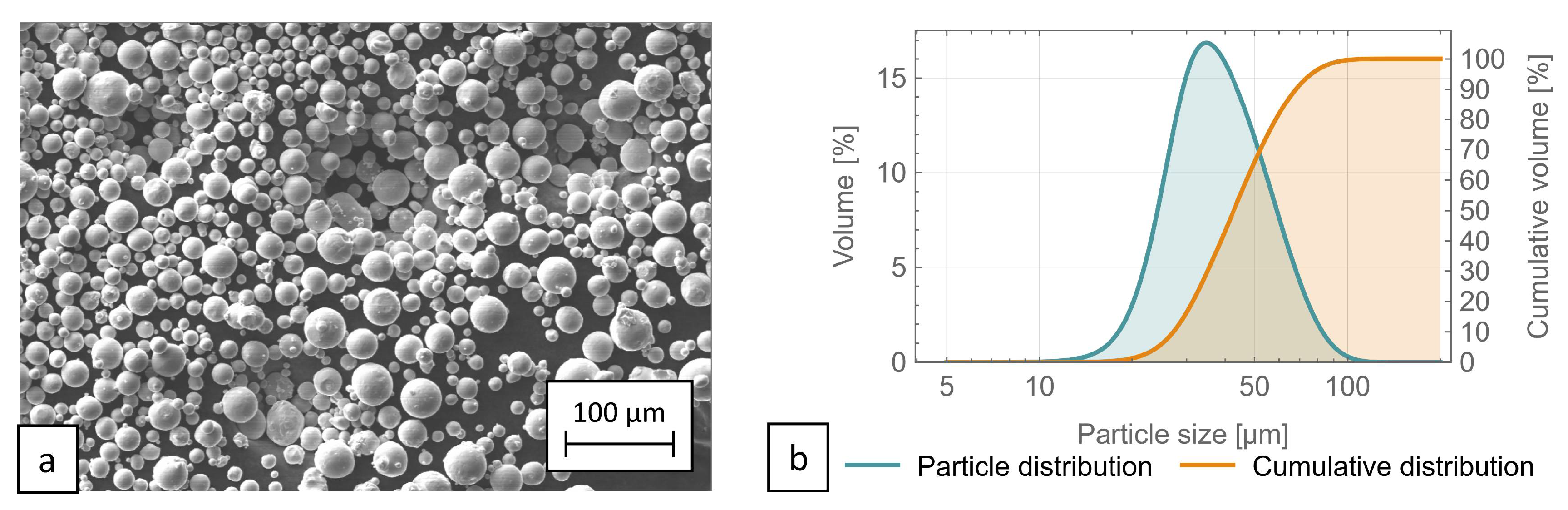
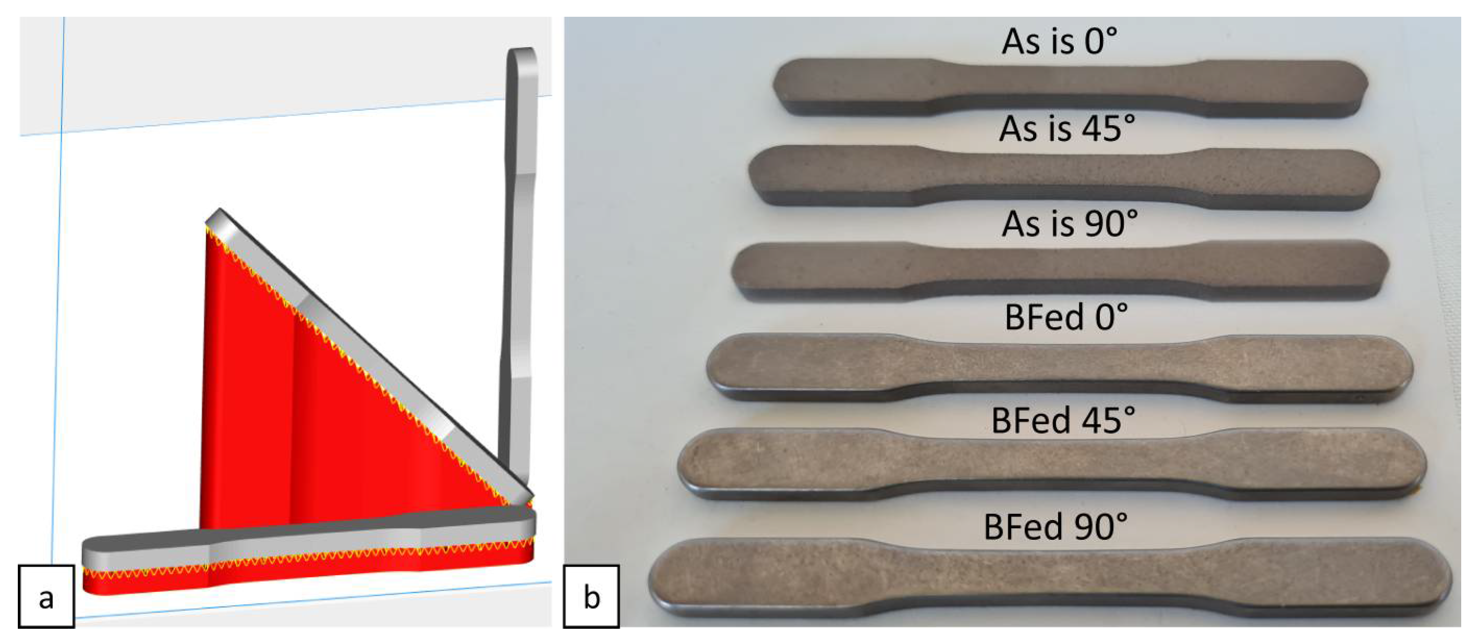
2.2. Fabrication Method

The SLM specimens used in this work were produced using an EOSINT®M290 machine (EOS GmbH, Krailling, Germany). The building volume of the mentioned printer is 250 × 250 × 325 mm3, the laser is a 400-W ytterbium fiber continuum laser, and the diameter of the beam spot is 100 μm. The printing process was carried out in an inert atmosphere using argon containing less than 0.1% oxygen. In order to reduce the effect of residual stresses, the building platform was preheated to 200 °C.
The material used in the case studies is Ti4Al6V, supplied by EOS [37], which is a widely used material for metal AM characterized by the chemical composition reported in Table 2.
Figure 2a shows the morphology of the titanium powder. The particles are almost spherical, with a variety of diameter sizes. The volume distribution of equivalent diameters is asymmetrical (blue curve), and the corresponding cumulative volume (orange curve) is characterized by the following metrics: d 10 , d 50 , and d 90 , which are the intercepts for 10%, 50%, and 90%, paired to 26.2 μm, 34.8 μm, and 71.3 μm, respectively.
The processing parameters are set according to the EOS standard directive for this material. The layer thickness is set at 30 µm, and the consecutive layers are rotated by 67° to minimize out-of-plane distortion. A stripes strategy is used for scanning, subdivided into internal and external scanning. The former is the hatch infill, which gives the part bulk resistance. The latter is more relevant to the scope of this paper because it characterizes the external surface. The bottom and top layers of the part are scanned through the so-called upskin and downskin, respectively. The lateral side is consolidated by using the contour strategy, which provides a set of parameters with the aim of improving the final part surface. The set of parameters is indicated in Table 3. Abrasive cutting is then used to detach the specimen from the building platform.

2.3. Secondary Finishing

BF is a mass finishing technology that permits deburring, generation of corner radii, part cleaning by removing rust, and surface finishing [38]. The process is performed via an octagonal rotating barrel filled with a charge composed of parts, media, water, and compound. When the barrel rotates, the charge is moved upward until a critical angle is reached; therefore, a layer called the active layer slides down, resulting in a relative velocity between parts and media, generating a delicate abrasion and microremoval of material [28]. Fixturing of the parts during the process is not required; hence, this process is suitable for components with a variety of sizes, shapes (also complex), and materials, such as AM components [39]. The main BF process parameters are the filling percentage and the rotational speed [40]. Depending upon these two parameters, six different motions, namely sliding, slumping, rolling, cascading, cataracting, and centrifuging, can occur inside the barrel [41]. Only two motions, i.e., rolling and the cascading, permit the microremoval of material. The rolling regime is characterized by slower rotational velocities and results in a more delicate action than the cascading regime. In [29], it was observed that the cascading motion achieves the same results as the rolling regime in a quarter of the working time.
In this experiment, a Rotar EMI 47 (ROTAR PRECISION MACHINERY INDUSTRIAL CO., LTD., Taichung City 411, Taiwan) machine characterized by an inclined octagonal barrel with a diameter of 400 mm is employed. It is equipped with an asynchronous motor with electronic speed control to permit its rotation. The employed media are composed of a matrix of synthetic resin and a mix of alumina, silica, and silicon carbide powders as abrasive. They are suitable to process metal components. They present an angled-cut, cylindrical shape with a diameter of 15 mm and a height of 25 mm. The BF process parameters, i.e., the rotational speed and the barrel-filling percentage, are chosen in order to guarantee, for this specific charge, the rolling and cascading motions. Considering the expertise of the authors, the filling percentage is fixed at 50% of the barrel volume; 30 and 42 rpm rotational speed values are considered for the rolling and cascading motions, respectively.

3. Results

3.1. First Case Study

In this case study, the surfaces of three Ti6Al4V tensile test specimens fabricated by SLM with three different building angles (0°, 45°, and 90°) are analyzed before and after BF conditioning.
Figure 3a shows the EOS preprocessing environment, namely the EOS Print 2.4 (EOS GmbH, Krailling, Germany), which allows for orientation of the parts (colored in grey) on the building platform and design of the support structures (colored in red). A selection of SLMed specimens for different building orientations is shown in Figure 3b. A significant improvement can be observed between the original specimen (as is) and that after conditioning (BFed).
Figure 4 shows the 3D map achieved by the system at a 0° building orientation. It reflects a typical outcome of the SLM fabricated part. As it is a horizontal surface, laser scanning is performed perpendicularly to the area; hence, the texture is predominantly composed of laser tracks and is highly visible in this case. Some profiles were extracted to highlight the limit of traditional roughness analysis on objects fabricated via SLM. The separation between small-scale and long-scale contributions, namely the roughness and the waviness, was determined via Gaussian filtering according to ISO 16610-21 [36]. The roughness profile was used to calculate the traditional R parameters [42]. For profile A, the calculated Ra is 4.24 µm, which is very close to the Rq value, highlighting a regular profile. The shape is symmetrical, as confirmed by an Rsk value close to 0, and slightly leptokurtic (Rku equal to 3.19). The spacing is expected to equal the value of the hatch distance (0.14 mm). The measured value of 0.155 mm confirms this theoretical aspect, considering that the measure is slightly inclined with respect to the scanning direction. However, this profile cannot describe the SLM behavior. In fact, by taking profile B, the measured Ra is almost three times the previous outcome, with doubled peak-to-valley height (Rt). The shape is deformed; the height distribution is asymmetrical and platykurtic. Additionally, the spacing markedly increased to the value of 0.260 mm. The Dq, which is an indication of the reflectiveness of the surface, is unchanged, as the increase in Ra is equal to the increase in spacing. In profile C, the spacing is increased, as expected, as the direction of the measure is taken almost parallel to the scanning strategy. However, the amplitude and shape parameters, which are mathematically unaffected by the measure direction, are changed again; the height distribution is markedly platykurtic, with Ra, Rq, and Rt at intermediate values with respect to the previous profiles. The Dq of this profile is markedly reduced in this case.
A surface inclined by 45° with respect to the stratification direction is shown in Figure 5. It is well-known that this angle affects the part quality. Profiles A, B, and C are extracted in different zones and show very different roughness parameters. In this case, the spacing changes considerably, as well as the shape of the height distribution; the balling effect is expected to result in chaotic behavior. In profile A only, the distribution is close to the Gaussian type. The most used parameter, Ra, changes by more than 50% around its mean value. In this case, the Dq value is low, along with the vertical measurement.
The previous analysis points out that single measurements taken on an SLM surface are not enough to adequately describe the quality. Thus, the non-homogeneity of the surface must be characterized via areal analysis carried out on 3D maps.
The data are arranged in an x-y-z array and graphed in a pseudo-color view, as reported in Figure 6a. It is evident that the surface is not homogeneous, with depressed areas and peaked zones. However, the height distribution is symmetrical, as confirmed by the Ssk parameter, with a value very close to zero. The Sku parameter indicates that this distribution is Gaussian. Hence, the Sv and Sp are expected to be similar. This is confirmed by the outcome. The values of the calculated parameters are reported in Table 4.
However, this description does not describe the previously evidenced texture due to the laser tracks. By calculating the autocorrelation function, it is possible to determine in which direction this function quickly decays. Figure 6c shows a polar plot of the main directions; 72.43° represents the most prominent direction. It is evident that this is exactly the direction with which the laser tracks are aligned. Other determined directions are 90.01° and 84.74°, with lower amplitude. The Sal and Str parameters are calculated as 0.25 mm and 52.94%, respectively, highlighting a marked anisotropy, as expected.
SLM fabricated surface rarely present with sufficient quality for functional application. Thus, a secondary finishing operation is required. The BF can be joined with the SLM due to the benefit of geometrical complexity freedom. The surface improvement is generally provided by material removal; hence, such characterization is of decisive importance.
The functional parameters consist of a cumulative sum of height cuts at specific points derived from the Abbot curve. Figure 7a is an example of thresholding the data at two specific points. Assume that the removal action removes all the peaks above 70% of the height range, and in a second moment, an additional 20% is removed. Red and green colors represent these ideal removal operations, whereas the blue color indicates the left area. The material removal is not homogeneous and cannot be approximated to a horizontal planar cut. Thus, it is important to quantify how material removal is achieved. The functional parameters are represented in Figure 7b within the Abbot curve, and their values are reported in Table 5. The Vmp, i.e., the peak material volume, represents the volume of material at a certain areal material ratio (the standard suggests 10%). In this case, this parameter is 0.00035 mm3/mm2. The parameter Vvv represents the volume of the valleys and is conventionally set at 80% of the areal material ratio. The obtained value is 0.0009182 mm3/mm2. These parameters are useful to understand the removal efficiency. In the case of BF, because the action takes place mainly on the peaks, a more impressive reduction in Vmp than Vvv is expected. Additionally, when the valleys are affected by the operation, conditioning should be stopped, or the surface can be damaged.
When BF takes place, the surface is considerably modified. After 12 h processing time, the previous texture is no longer visible, and only a few traces are recognizable (Figure 8a). This provides a homogeneity to the surface, as evidenced by the polar plot shown in Figure 8b. Multiple low-intensity angles are the main indications that the SLM fingerprint is going to be eliminated. Accordingly, the isotropy is increased at 66.73%. The volume analysis indicates that the peaks are markedly reduced, and the valleys begin to be altered (Figure 8c). At 24 h, almost all the previous traces are eliminated. Figure 8d highlights three main bumps (colored in green). Depression can also be observed in the top-right part of the image. Analysis of the directions (Figure 8e) confirms a slight improvement in the Sal and Str parameters, with an isotropy value of 70.80%. At this processing time, volumetric analysis indicates that the valleys are considerably reduced, suggesting that they are affected by the BF tools (Figure 8f). In this case, further conditioning can cause damage due to microfatigue and microcracking phenomena.
As expected, after 48 h processing time, some issues occur. Few defects are present in zones previously unaffected by bumps (Figure 9a). Moreover, defects have a new shape (elongated), and the previously mentioned depression is more evident. As a result, the anisotropy is markedly reduced, as highlighted by the Str parameter (22.25%). The spectrum polar plot indicates a host of directions with high amplitude (Figure 9b). This condition is typical of deformed surfaces. Flatness analysis can measure this deviation, indicating when to stop the operation. The FLTq parameter at this working time is increased by 35% with respect to the previous time. This could be due overconditioning phenomena, which cause damage and alter the waviness of the surface. This is confirmed by volumetric analysis; the Vvv value is further decreased, and the Vmp is now increased (Figure 9c). This indicates that the valleys are now conditioned, but new peaks are formed. In order to investigate different BF effects, the rotational speed is reduced to understand whether a more delicate action can improve the flatness. Figure 9d is the surface false-color visualization at 48 h with a reduced barrel rotational speed. The outcome shows new local bumps. The Sa is the same as in the previous case, but the anisotropy is increased, leading to an Str value of 64.54% (Figure 9e). In this case, the flatness is improved, as confirmed by an FLTq value close to that at 24 h working time, with a high rotational speed. Volumetric analysis indicates alterations similar to those in the previous case (Figure 9f). In conclusion, a low rotational speed after 48 h can provide flatness quality and an Sa value equal to that in the high-speed case at 24 h; therefore, this is not convenient, and the speed must be limited to the 24 h value, or the damage of the action may induce anisotropy and a lack of flatness.
The previous analysis can be repeated for the 45° and 90° building orientations, with some differences in terms of the outcomes.
Figure 10a–d shows the 3D maps for the 45° build orientation at different working times. The initial morphology is uniform with high isotropy (Str = 56%). After 12 h, the peaks are markedly reduced, and the surface appears to be more planar. However, flatness analysis shows that the quality is not improved at this stage, as the remaining peaks are non-uniform. The flatness is improved at 24 h, with only some bumps still present. At 48 h, the 0° issues are apparently resolved.
The 90° slope shows a similar trend, as reported in Figure 11a–d. In the beginning, the surface is characterized by a high density of peaks that are probably difficult to remove. At 12 h and 24 h, the density of bumps is higher than in the 45° case at the same time. However, they appear to be completely removed after 48 h. Evaluation of the areal parameters indicates both differences and similarities between the investigated building orientations.
The Sa trends are shown for the various slopes in Figure 12a. Notwithstanding the different starting Sa values, all the surfaces are reduced to about 1 µm after 24 h. After 48 h, a slight improvement is observed for 45° and 90°, whereas the 0° Sa value remains unchanged. The Str values of the analyzed surfaces are similar to those before BF employment (Figure 12b). As previously described, the 0° surfaced is subjected to an isotropy improvement for the first 24 h. Conversely, after 48 h, the isotropy dramatically decreases to a value less than that measured at the beginning of the process. The 45° surface presents with a descending in the first 24 h, returning to its starting value only when all the traces are deleted. The 90° surface presents with a slightly decreasing trend after an initial improvement, signaling that the underlying defects of SLM and that the operation should be stopped. Analysis of the peak volume (Figure 12c) confirms the action of BF, which gradually alters the profiles from the top to the bottom. As previously mentioned, only the 0° surface shows an opposite trend at 48 h; therefore, the operation should be stopped at the previous time step. This issue is indicated by the FLTq value: up to 24 h, it decreases, indicating satisfactory processing; at 48 h, the flatness is worsened by new local new damage (Figure 12d). The 45° case, as discussed, requires more than 12 h to achieve an improvement, after which the trend is reverses; therefore, 48 h processing time assures the best result. The 90° slope is characterized by a continuous improvement in flatness.
As a conclusive investigation, the as is SLMed surfaces at the investigated building angles are compared by means of the calculated areal parameters. Figure 13a shows the values of Sa ad Sz. As expected, the trends increase with the building angle; however, the rate of increase of Sz is greater than that of Sa. In other words, the wider the building angle, the greater the ratio between Sz and Sa. This indicates that inclined surfaces are more affected by deeper and/or higher defects than horizontal surfaces, where the laser perpendicularly processes the surface. With respect to isotropy (Figure 13b), Sal parameter differs considerably at all investigated angles. The Sal indicates the minimum distance at which similar structures can be observed. At 0°, the texture is mainly characterized by tracks with few local defects and a Sal value of 0.25 mm. At 45° and 90°, the balling phenomenon becomes predominant, reducing this minimum distance, as confirmed by the low Sal values. Conversely, the Str highlights similar measures of the surface isotropy for all investigated angles. The volumetric analysis is summarized in Figure 13c. As the height parameters increase with the building angles, the volumetric parameters (Vmp and Vmc) increase accordingly. The ratio between Vmp and Vmc indicates the relative volume of the surface peaks with respect to the core. As evidenced by the graph, the 0° surface is characterized by a smaller peak relative volume than the other inclined surfaces. This indicates that fewer peaks need to be removed in the subsequent finishing operations from the starting profile; accordingly, a heavier or faster operation is required for inclined surfaces. The comparison via flatness analysis shows that the outcomes for the selected building angles differ slightly (Figure 13d); the worst case is the 0°, and the best result is obtained for the 45° angle.

3.2. Second Case Study

A complex geometry is fabricated for the second part of this case study. The part is shown in Figure 14. Maps are generated of the outer and inner surfaces in order to evaluate the different actions provided by BF. The limited access to internal zones may reduce the efficiency of the operation, as the process is based on granular flow.
The maps were generated after fabrication and at the same working times as in the previous case, namely 12 h, 24 h, and 48 h, with additional extensions at 60 h and 96 h to investigate possible issues or completion using the slow rotational speed.
Figure 15a–d shows maps for the external zones. The evolution complies with the previous behaviors. The as-is surface (Figure 15a) is characterized by high peaks and valleys, which are markedly reduced after 24 h BF (Figure 15b). After 48 h, deletion of the SLM fingerprint is complete; only small valleys can be observed from in map shown in Figure 15c. The working time is extended to 96 h to analyze possible issues; only a slight improvement is observed in the 3D maps (Figure 15d).
As expected, slower modifications are observed in the internal zones. The 3D map before BF is shown in Figure 16a. The morphology is similar to that of the external zone, as SLM processing does not distinguish between wall faces (Figure 16a). After 24 h, the highest peaks are removed, but the action is evidently slower than before (Figure 16b). The peak-to-valley height is only marginally reduced. At 48 h, the valleys are still not affected by the operation; thus, further action is expected to provide an improvement. The motivation is clarified if the valley sizes are considered; they are smaller than the media size, so they cannot be conditioned (Figure 16c). If a very long working time is employed, a further improvement is obtained, as shown in Figure 16d.
The areal parameters quantify the previous observations. The Sa trends reported in Figure 17a highlight varying exponential decays for the analyzed zones: at 48 h, the external zones reach the 0.5 µm plateau, whereas the internal zones require twice the working time to achieve a value of 2.4 µm. Analysis of the anisotropies allows for deduction of some considerations. The Sal behavior confirms the trend observed in the tensile test specimens; in the beginning, conditioning increases the isotropy by cutting the highest peaks, and the operation reveals underlying anisotropic shapes of the surface (Figure 17b). Different speeds are observed for external and internal zones. The Str parameter indicates a global isotropy that is slowly decreasing for the internal surface, but a limit must be evidenced for the external surface (Figure 17c). After 60 h, the isotropy trend is inverted, indicated that some new local defects are created, as reported for the 0° case. This suggests that the operation should be stopped in advance. The graph in Figure 17d concerns the flatness trends; after only 24 h, the a satisfactory result is obtained on the external surface, with a slight increases at 60 h for the previously stated reasons. The flatness of the internal surfaces is constantly reduced because the operation continues to remove material from the peaks, and valleys are not still reached. Two possible solutions for these contrasting needs can be proposed. The first option is to select a working time that balances the attainable quality in accordance with the demands of the application (maximum Sa, uniformity, and flatness). A more complicated solution is to stop the BF machine when the optimal result is achieved in the external zones, selectively cover these zones, and restart the process to complete the internal zones.

4. Conclusions

The results presented in this work reveal the capability of areal analysis when applied to objects produced by SLM. The selected case studies underline how the application of a secondary finishing operation, such as BF, can be investigated in depth, providing many important processing indications.
The obtained results led to the following conclusions:
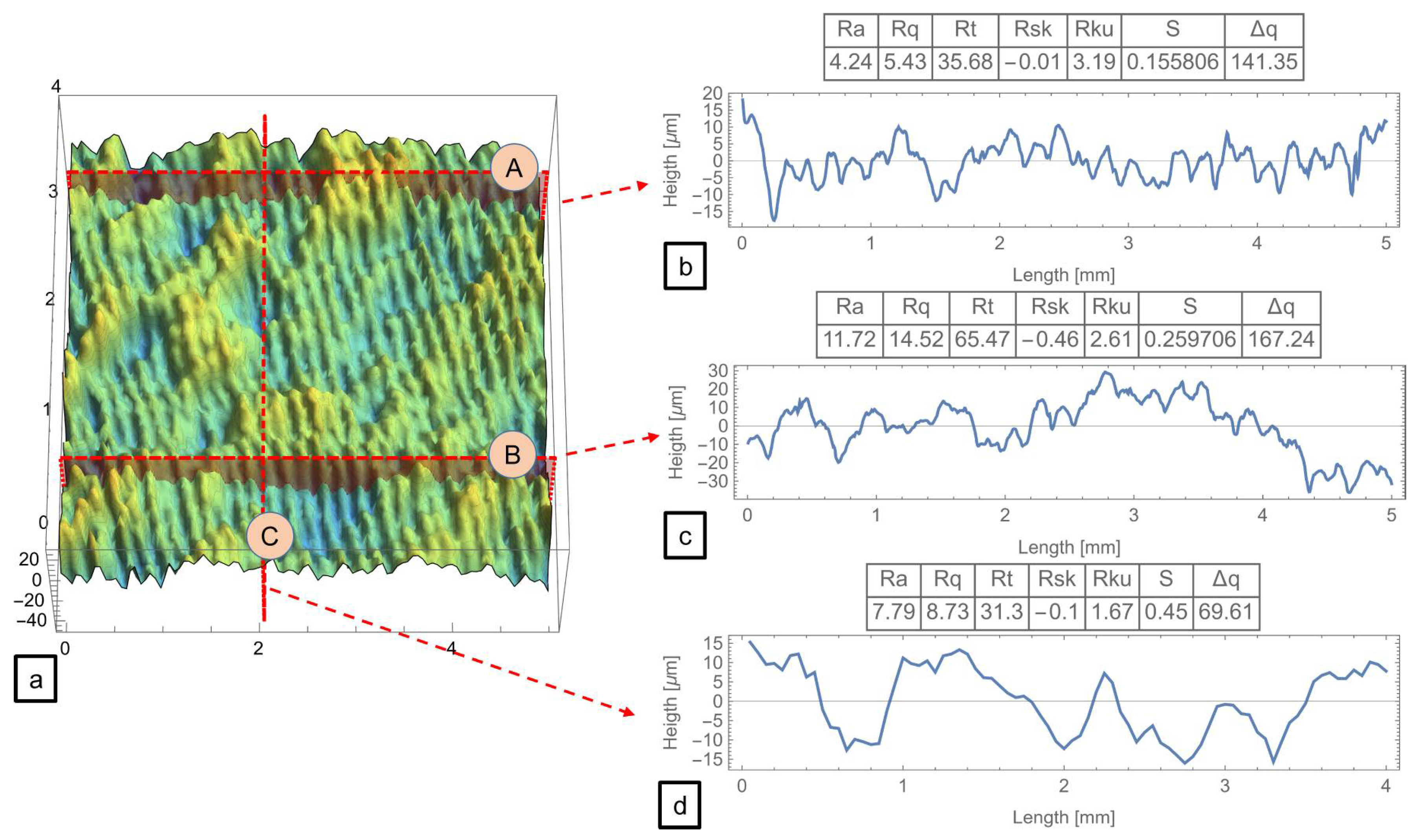
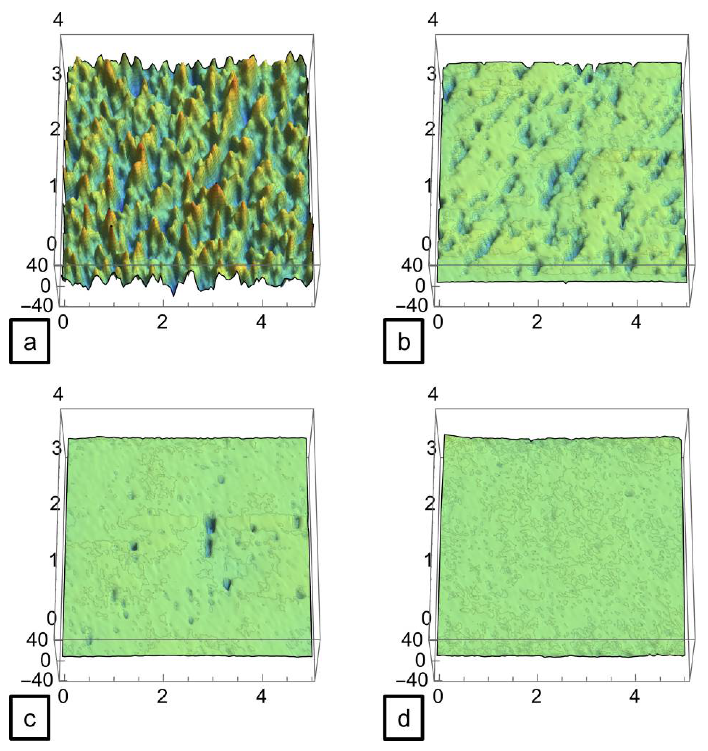
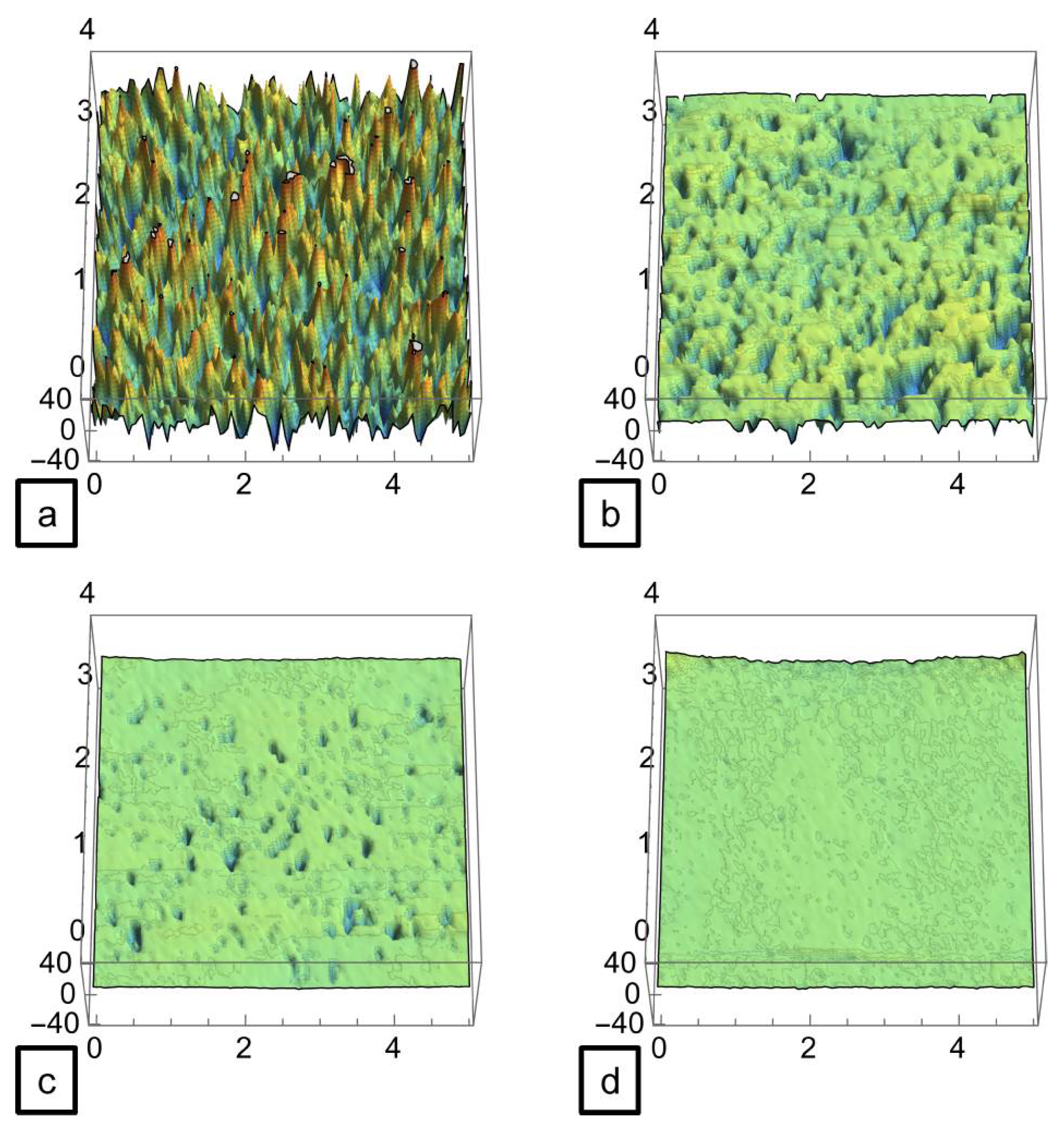
  • The use of 2D roughness analysis is not sufficient to describe the texture of SLMed surfaces, they exhibit non-homogeneities and anisotropies;
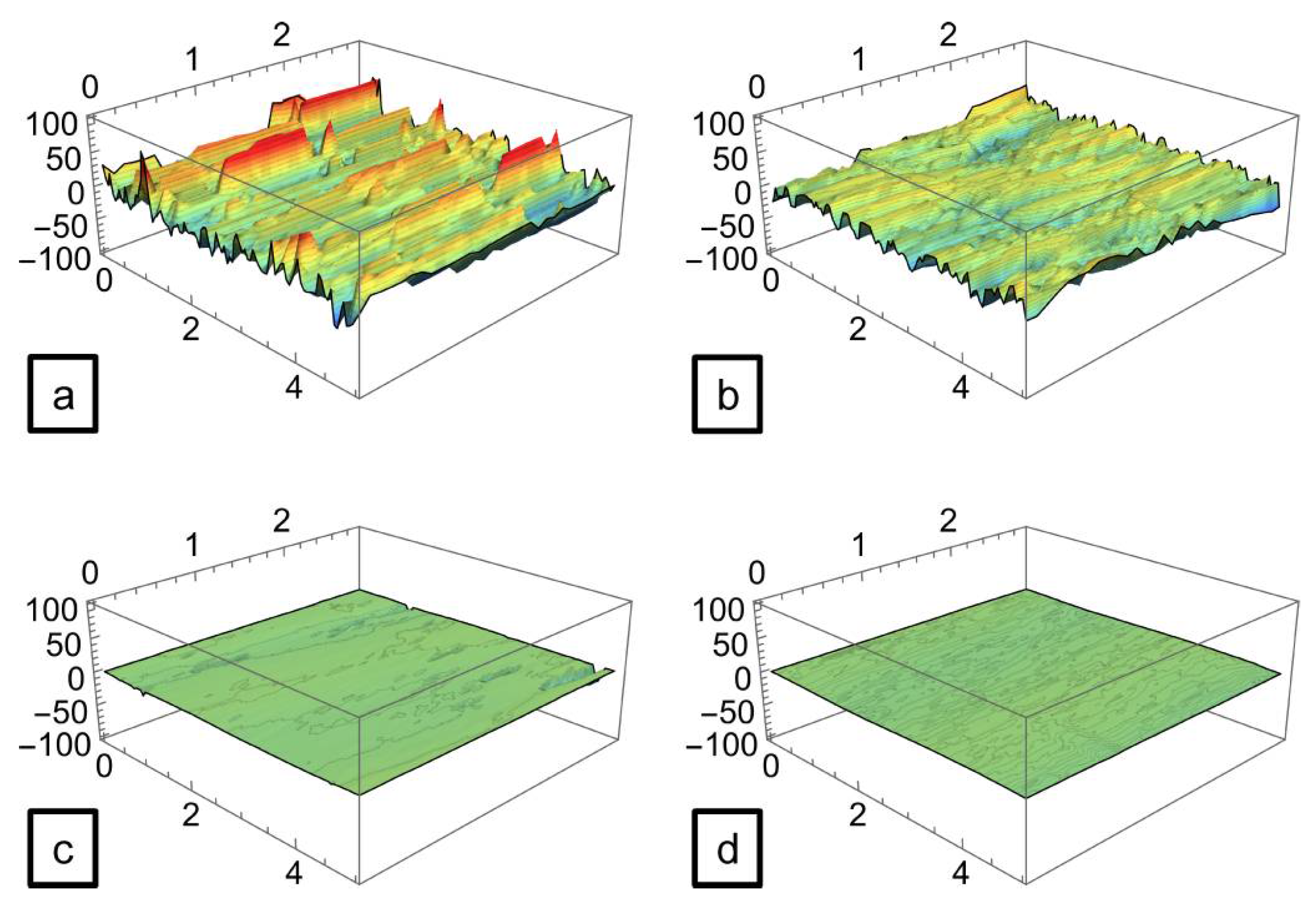
  • The application of BF allows for improvement of the surface quality, but different building orientations result in differing starting surface textures with varying evoltions, as demonstrated by conditioning;
  • Volume analysis confirms the BF mechanism, which is characterized by a marked reduction in the average peak volume, whereas the valleys are only slightly modified;
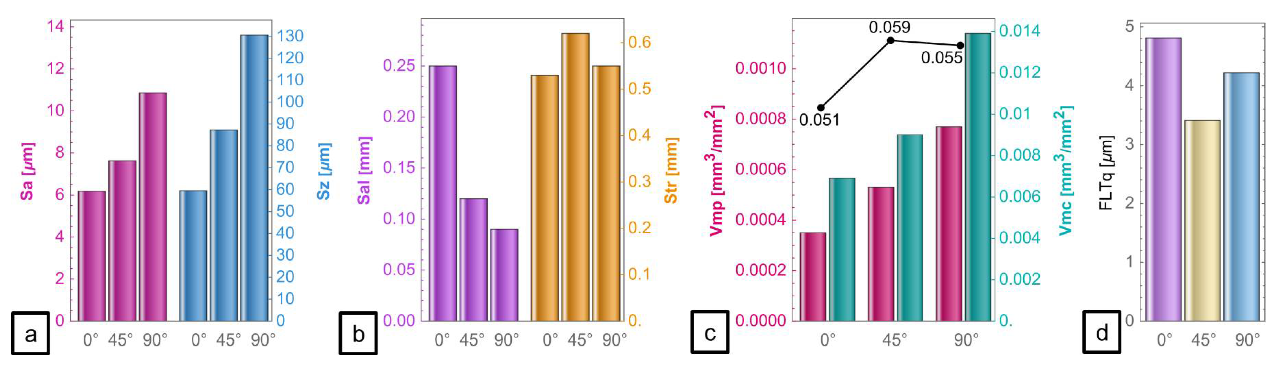
  • In the case of 0° surfaces, satisfactory isotropy and height parameters are obtained after 24 h. Beyond this time, functional analysis reveals that the valleys are altered, and new damage occurs. Flatness analysis reveals an increase in the FLTq parameter, suggesting that BF should be stopped at 24 h;
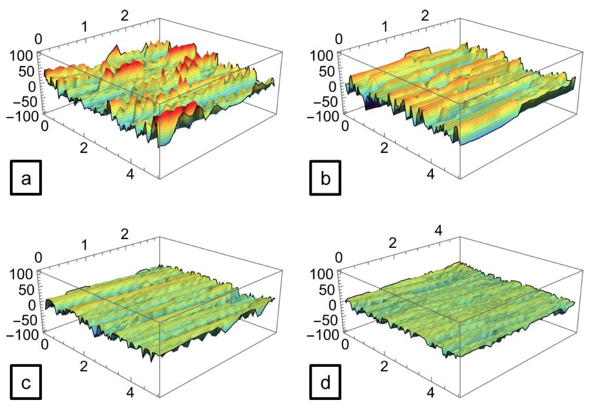
  • Conversely, 45° and 90° surfaces require the longest investigated processing time to achieve good surface quality;
  • The application of a slower BF rotational speed results in a more delicate action, as the rolling motion takes place within the barrel. Analysis indicates that the result after 48 h are the same as those achieved by BF at high speed after 24 h, making it a non-economic choice;
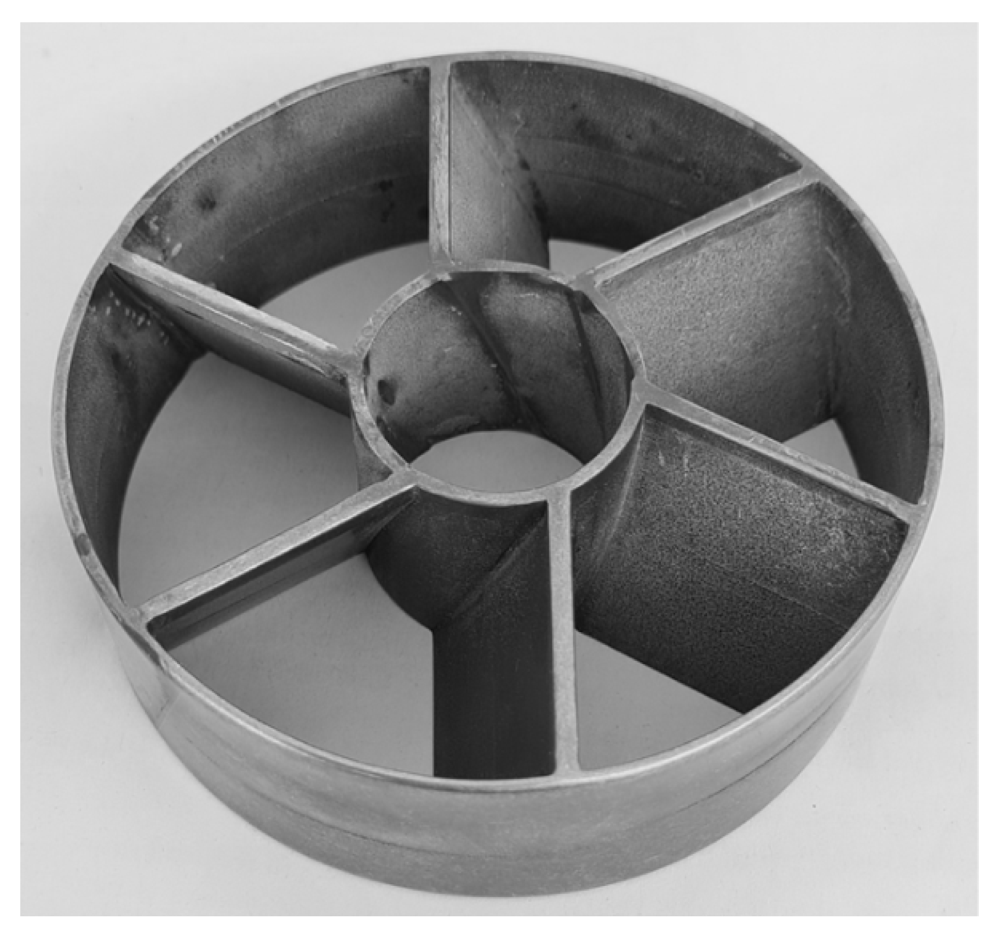
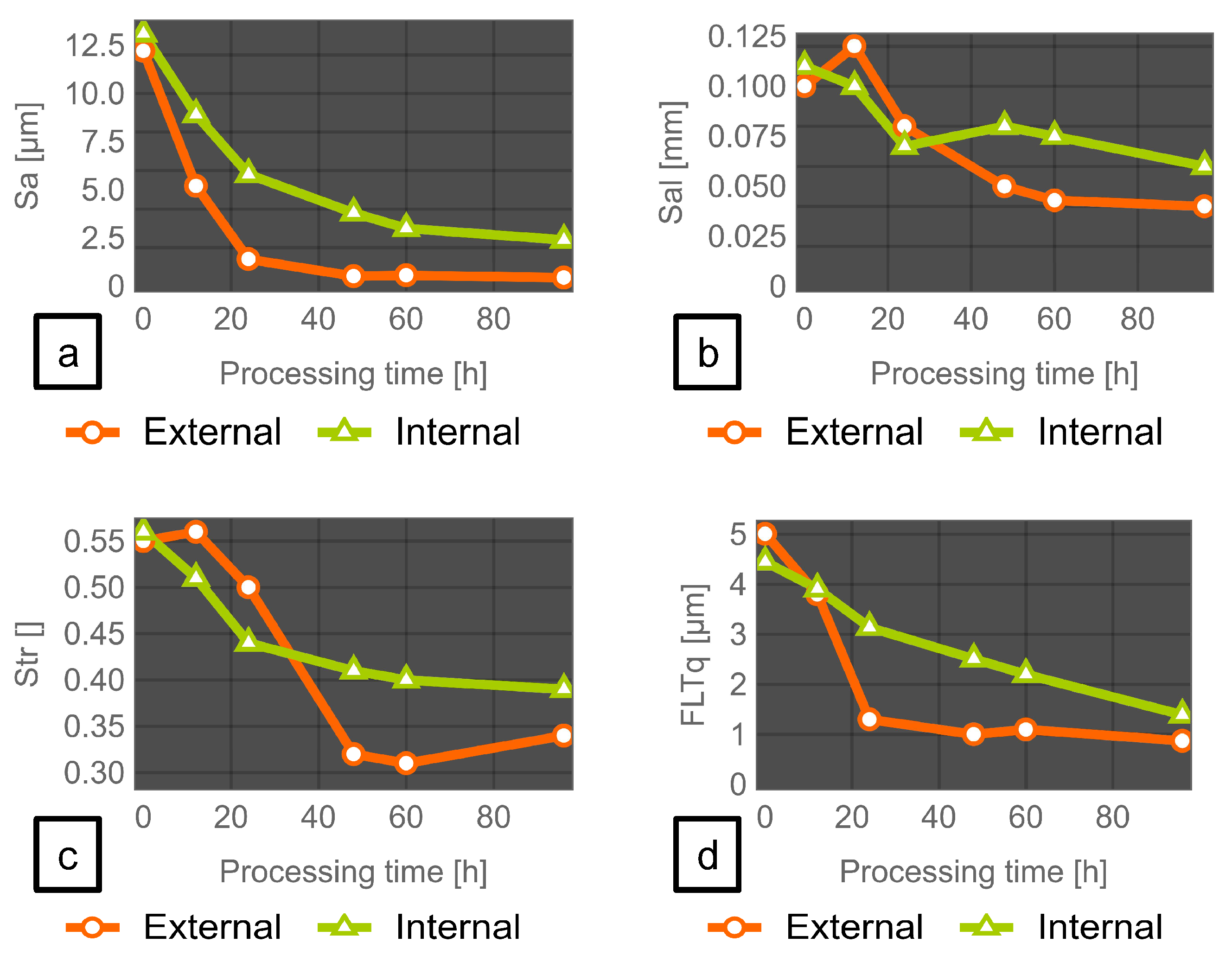
  • The second case study involves a complex geometry. External surfaces confirm the results obtained for a simple geometry in terms of height parameters, volume analysis, and isotropy;
  • The internal surfaces undergo slower decay of the areal parameters due to the reduced accessibility of the measured zone. As a consequence, the processing time must be extended for internal surfaces.

Author Contributions

Conceptualization, A.B., L.B. and N.G.; methodology, A.B., L.B. and N.G.; software, A.B. and N.G.; validation, A.B. and L.B.; formal analysis, A.B., L.B. and N.G.; writing—original draft preparation, A.B., L.B. and N.G.; writing—review and editing, A.B., L.B. and N.G.; supervision, A.B. and L.B. All authors have read and agreed to the published version of the manuscript.

Funding

This research received no external funding.

Institutional Review Board Statement

Not applicable.

Informed Consent Statement

Not applicable.

Data Availability Statement

The study did not report any data.

Conflicts of Interest

The authors declare no conflict of interest.

References

  1. Gibson, I.; Roson, D.; Stucke, B. Additive Manufacturing Technologies, 2nd ed.; Springer Science Business Media: New York, NY, USA, 2015; ISBN 978-1-4939-2113-3. [Google Scholar]
  2. ISO/ASTM 52900-15; Standard Terminology for Additive Manufacturing—General Principles—Terminology. ASTM International: West Conshohocken, PA, USA, 2015.
  3. Kunze, K.; Etter, T.; Grässlin, J.; Shoklover, V. Texture, anisotropy in microstructure and mechanical properties of IN738LC alloy processed by selective laser melting (SLM). Mater. Sci. Eng. A 2015, 620, 213–222. [Google Scholar] [CrossRef]
  4. Gu, D. Laser Additive Manufacturing of High-Performance Materials, 1st ed.; Springer: Berlin/Heidelberg, Germany, 2015; ISBN 978-3-662-46089-4. [Google Scholar]
  5. Yang, Y.; Loh, H.T.; Fuh, J.Y.H.; Wang, Y.G. Equidistant Path Generation for Improving Scanning Efficiency in Layered Manufacturing. Rapid Prototyping J. 2002, 8, 30–37. [Google Scholar] [CrossRef]
  6. Shi, Y.; Zhang, W.; Cheng, Y.; Huang, S. Compound Scan Mode Developed from Subarea and Contour Scan Mode for Selective Laser Sintering. Int. J. Mach. Tools Manuf. 2007, 47, 873–883. [Google Scholar] [CrossRef]
  7. Hashmi, S.; Batalha, G.F.; van Tyne, C.J.; Yilbas, B.S. Comprehensive Materials Processing, 1st ed.; Elsevier Science Ltd.: Waltham, MA, USA, 2014; ISBN 978-0-080-96532-1. [Google Scholar]
  8. Tromme, E.; Kawamoto, A.; Guest, J.K. Topology optimization based on reduction methods with applications to multiscale design and additive manufacturing. Front. Mech. Eng. 2020, 15, 151–165. [Google Scholar] [CrossRef]
  9. Rombouts, M.; Kruth, J.P.; Froyen, L.; Mercelis, P. Fundamentals of Selective Laser Melting of alloyed steel powders. CIRP Ann. 2006, 55, 187–192. [Google Scholar] [CrossRef]
  10. Stempin, J.; Tausendfreund, A.; Stöbener, D.; Fischer, A. Roughness Measurements with Polychromatic Speckles on Tilted Surfaces. Nanomanuf. Metrol. 2021, 4, 237–246. [Google Scholar] [CrossRef]
  11. Aboulkhair, N.T.; Simonelli, M.; Parry, L.; Ashcroft, I.; Tuck, C.; Hague, R. 3D printing of Aluminum alloys: Additive Manufacturing of Aluminum alloys using selective laser melting. Prog. Mater. Sci. 2019, 106, 100578. [Google Scholar] [CrossRef]
  12. Salak, A. Ferrous Powder Metallurgy, 10th ed.; Cambridge International Science Publishing: Cambridge, UK, 1995; ISBN 189-8-32603-7. [Google Scholar]
  13. Zhang, B.; Li, Y.; Bai, Q. Defect Formation Mechanisms in Selective Laser Melting: A Review. Chin. J. Mech. Eng. 2017, 30, 515–527. [Google Scholar] [CrossRef] [Green Version]
  14. Brodin, H.; Andersson, O.; Johansson, S. Mechanical testing of a selective laser melted superalloy. Proceeding of the 13th International Conference on Fracture, Beijing, China, 16–21 June 2013; pp. 2573–2574. [Google Scholar]
  15. Jinhui, L.; Ruidi, L.; Wenxian, Z.; Liding, F.; Huashan, Y. Study on formation of surface and microstructure of stainless-steel part produced by selective laser melting. Mater. Sci. Technol. 2010, 26, 1259–1264. [Google Scholar] [CrossRef]
  16. Li, R.; Liu, J.; Shi, Y.; Wang, L.; Jiang, W. Balling behavior of stainless steel and nickel powder during selective laser melting process. Int. J. Adv. Manuf. Technol. 2012, 59, 1025–1035. [Google Scholar] [CrossRef]
  17. Laleh, M.; Hughes, A.E.; Yang, S.; Li, Y.; Xu, W.; Gibson, I.; Tan, M.Y. Two and three-dimensional characterization of localized corrosion affected by lack-of-fusion pores in 316L stainless steel produced by selective laser melting. Corros. Sci. 2020, 156, 108394. [Google Scholar] [CrossRef]
  18. Kumar, L.J.; Pandey, P.M.; Wimpenny, D.I. (Eds.) 3D Printing and Additive Manufacturing Technologies, 1st ed.; Springer: Berlin, Germany, 2019; ISBN 978-981-13-0305-0. [Google Scholar]
  19. Sefene, E.M. State-of-the-art of selective laser melting process: A comprehensive review. J. Manuf. Syst. 2022, 63, 250–274. [Google Scholar] [CrossRef]
  20. Boschetto, A.; Bottini, L.; Pilone, D. Effect of laser remelting on surface roughness and microstructure of AlSi10Mg selective laser melting manufactured parts. Int. J. Adv. Manuf. Technol. 2021, 113, 2739–2759. [Google Scholar] [CrossRef]
  21. Aboulkhair, N.T.; Maskerya, I.; Tucka, C.; Ashcroft, I.; Everitt, N.M. On the formation of AlSi10Mg single tracks and layers in selective laser melting: Microstructure and nano-mechanical properties. J. Mater. Process. Technol. 2016, 230, 88–98. [Google Scholar] [CrossRef]
  22. Boschetto, A.; Bottini, L.; Veniali, F. Roughness modeling of AlSi10Mg parts fabricated by selective laser melting. J. Mater. Process. Technol. 2017, 241, 154–163. [Google Scholar] [CrossRef]
  23. Zaleski, K.; Skoczylas, A.; Brzozowska, M. The effect of the conditions of shot peening the Inconel 718 nickel alloy on the geometrical structure of the surface. Adv. Sci. Technol. Res. J. 2017, 11, 205–211. [Google Scholar] [CrossRef]
  24. Lesyk, D.A.; Martinez, S.; Mordyuk, B.N.; Dzhemelinskyi, V.V.; Lamikiz, A.; Prokopenko, G.I. Post-processing of the Inconel 718 alloy parts fabricated by selective laser melting: Effects of mechanical surface treatments on surface topography, porosity, hardness and residual stress. Surf. Coat. Technol. 2020, 381, 125136. [Google Scholar] [CrossRef]
  25. Avanzini, A.; Battini, D.; Gelfi, M.; Girelli, L.; Petrogalli, C.; Pola, A.; Tocci, M. Investigation on fatigue strength of sand-blasted DMLS-AlSi10Mg alloy. Procedia Struct. Integr. 2019, 18, 119–128. [Google Scholar] [CrossRef]
  26. Löber, L.; Flache, C.; Petters, R.; Kühn, U.; Eckert, J. Comparison of different post processing technologies for SLM generated 316l steel parts. Rapid Prototyp. J. 2013, 19, 173–179. [Google Scholar] [CrossRef]
  27. Kaynak, Y.; Kitay, O. The effect of post-processing operations on surface characteristics of 316L stainless steel produced by selective laser melting. Addit. Manuf. 2019, 26, 84–93. [Google Scholar] [CrossRef]
  28. Boschetto, A.; Bottini, L.; Macera, L.; Veniali, F. Post-Processing of Complex SLM Parts by Barrel Finishing. Appl. Sci. 2020, 10, 1382. [Google Scholar] [CrossRef] [Green Version]
  29. Boschetto, A.; Bottini, L.; Veniali, F. Surface roughness and radiusing of Ti6Al4V selective laser melting-manufactured parts conditioned by barrel finishing. Int. J. Adv. Manuf. 2018, 94, 2773–2790. [Google Scholar] [CrossRef]
  30. Leach, R. (Ed.) Characterization of Aerial Texture; Springer: Berlin/Heidelberg, Germany, 2013; Chapter 1; ISBN 978-3-642-36457-0. [Google Scholar]
  31. ISO 4287:2000; Geometrical Product Specification (GPS), Surface texture: Profile Method, Terms, Definitions and Surface Texture Parameters. International Organization of Standardization: Geneva, Switzerland, 2000.
  32. ISO 4288:1996; Geometrical Product Specifications (GPS), Surface Texture: Profile Method, Rules and Procedures for the Assessment of Surface Texture. International Organization of Standardization: Geneva, Switzerland, 1996.
  33. ISO 25178-2:2012; Geometrical Product Specifications (GPS), Surface Texture: Aerial, Part 2: Terms, Definitions and Surface Texture Parameters. International Organization for Standardization: Geneva, Switzerland, 2012.
  34. ISO 1011:2004; Geometric Product Specification (GPS), Geometrical Tolerancing, Tolerances of Form, Orientation, Location and Run-Out. International Organization for Standardization: Geneva, Switzerland, 2004.
  35. ISO 12781-1:2011; Geometrical Product Specification (GPS), Flatness, Part 1: Vocabulary and Parameters of Flatness. International Organization for Standardization: Geneva, Switzerland, 2011.
  36. ISO 16610-21:2012; Geometrical Product Specifications (GPS), Filtration, Part 21: Linear Profile Filters: Gaussian Filters. International Organization for Standardization: Geneva, Switzerland, 2012.
  37. Material Data Sheet EOS TitaniumTi4Al6V. Available online: https://www.eos.info/03_system-related-assets/material-related-contents/metal-materials-and-examples/metal-material-datasheet/titan/ti64/material_datasheet_eos_titanium_ti64_grade5_en_web.pdf (accessed on 15 July 2022).
  38. Tulinski, E.H. Mass finishing. In ASM Metals Handbook: Surface Engineering, 9th ed.; ASM International: Materials Park, OH, USA, 1994; Volume 5, pp. 261–277. ISBN 978-0-871-70011-7. [Google Scholar]
  39. Nalli, F.; Bottini, L.; Boschetto, A.; Cortese, L.; Veniali, F. Effect of Industrial Heat Treatment and Barrel Finishing on the Mechanical Performance of Ti6Al4V Processed by Selective Laser Melting. Appl. Sci. 2020, 10, 2280. [Google Scholar] [CrossRef] [Green Version]
  40. Gillespie, L.K. Mass Finishing Handbook, 1st ed.; Industrial Press Inc.: New York, NY, USA, 2007; ISBN 9780831132576. [Google Scholar]
  41. Henein, H.; Brimacombe, J.K.; Watkinson, A.P. Experimental study of transverse bed motion in rotary kilns. Metall. Trans. B 1983, 14, 91–205. [Google Scholar] [CrossRef]
  42. Gadelmawla, E.S.; Koura, M.M.; Maksoud, T.M.A.; Elewa, I.M.; Soliman, H.H. Roughness parameters. J. Mater. Process. Technol. 2002, 123, 133–145. [Google Scholar] [CrossRef]
Figure 1. Framework of the system (a) and measurement layout (b).
Jmmp 06 00083 g001
Figure 2. SEM photo (a) and granulometry analysis (b) of Ti6Al4V.
Jmmp 06 00083 g002
Figure 3. Specimen models and support structures; (a) fabricated specimens; (b) for different building orientations before and after the BF employment.
Jmmp 06 00083 g003
Figure 4. 3D surface map at 0° slope (a): profiles A (b) and B (c) extracted horizontally and profile C extracted vertically (d).
Jmmp 06 00083 g004
Figure 5. 3D surface map at 45° slope (a): profiles A (b) and B (c) extracted horizontally and profile C extracted vertically (d).
Jmmp 06 00083 g005
Figure 6. Pseudo-color view of the 0° slope surface: (a) histogram and Abbot curve (b), as well as polar spectrum graph (c).
Jmmp 06 00083 g006
Figure 7. Threshold analysis (a) and volume parameters (b).
Jmmp 06 00083 g007
Figure 8. Analysis of the 0° slope surface after 12 h working time: false color map (a), isotropy analysis (b), and functional analysis (c). Analysis of the same slope after 24 h: false color map (d), isotropy analysis (e), and functional analysis (f).
Jmmp 06 00083 g008
Figure 9. Analysis of the 0° slope surface after 48 h working time: false color map (a), isotropy analysis (b), and functional analysis (c). Analysis of the same slope after 48 h with a slow rotational speed of the barrel: false color map (d), isotropy analysis (e), and functional analysis (f).
Jmmp 06 00083 g009
Figure 10. 3D maps of 45° building orientation surfaces before BF (a), after 12 h (b), after 24 h (c), and after 48 h (d) working time.
Jmmp 06 00083 g010
Figure 11. 3D maps of 90° building orientation surfaces before BF (a), after 12 h (b), after 24 h (c), and after 48 h (d) working time.
Jmmp 06 00083 g011
Figure 12. Trends of areal parameters for investigated building orientations: Sa (a), Str (b), Vmp (c), and FLTq (d).
Jmmp 06 00083 g012
Figure 13. Areal roughness parameters for investigated building orientations: Sa vs. Sz (a), Sal vs. Str (b), Vmp vs. Vmc, and Vmp-to-Vmc ratio (c), and FLTq (d).
Jmmp 06 00083 g013
Figure 14. SLMed propeller for case study 2.
Jmmp 06 00083 g014
Figure 15. Propeller external SLMed surface after (a) 24 h (b), 48 h (c), and 96 h (d) BF working time.
Jmmp 06 00083 g015
Figure 16. Propeller internal SLMed surface after (a) 24 h (b), 48 h (c), and 96 h (d) BF working time.
Jmmp 06 00083 g016
Figure 17. Trends of areal parameters for external and internal zones of the propeller for different BF working times: Sa (a), Sal (b), Str (c), and FLTq (d).
Jmmp 06 00083 g017
Table 1. Profilometer datasheet.
Vertical HeightVertical PrecisionTip RadiusTravel SpeedVertical ForceTravelling Distance
2400 µm16 nm2 µm0.5–2 mm/s0.75 mN50 mm
Table 2. Ti4Al6V mechanical properties.
Chemical CompositionALVFeCNHOTi
Ti6Al4V (wt.%)5.5–6.83.5–4.5≤0.30≤0.08≤0.05≤0.015≤0.20Balanced
Table 3. Exposure parameters for Ti6Al4V.
Power
(W)
Scan Speed
(mm/s)
Hatch Distance
(mm)
Contour Offset
(mm)
Hatch infill28012000.14-
Hatch upskin28012000.14-
Hatch downskin12010000.10-
Contour1501250-0.02
Table 4. Primary surface, spatial parameters, and functional parameters for the 0° slope surface.
Height ParametersSpatial Parameters
SaSqSskSkuSpSvSzSalStr
6.1827.809−0.045683.10528.1131.4359.540.25290.5294
µmµm µmµmµmmm
Table 5. Functional parameters for the 0° slope surface.
VmVvVmpVmcVvcVvv
0.00035330.010450.00035330.0069080.0095340.0009182
mm³/mm²mm³/mm²mm³/mm²mm³/mm²mm³/mm²mm³/mm²
Publisher’s Note: MDPI stays neutral with regard to jurisdictional claims in published maps and institutional affiliations.

