1. Introduction
In recent years, unmanned aerial vehicles (UAVs) have developed significantly in agricultural production, including application such as scenarios spraying pesticides and herbicides, spreading fertilizers, seeding, and farmland monitoring, etc. [
1,
2]. Whether the UAV continues to work needs to be determined by judging whether there is still material in the storage tank. The controller unit carried by the UAV needs to determine whether the amount of material currently released is accurate using the mass flow rate. Therefore, it is essential to accurately monitor the allowance and the mass flow rate of the storage tank for the operation accuracy of the UAV in the process of releasing particulate materials [
3].
In the existing scientific research, according to the different principles, the monitoring quantity and mass flow rate can be divided into four methods. The first method is the photoelectric method. In the study of this method, Swisher et al. designed an optical sensor for measuring fertilizer flow based on the laser light source. The sensor consisted of 32 photoelectric tubes. The instantaneous flow rate of the fertilizer was obtained according to the shielding strength of particles to light [
4]. Grift et al. previously examined the correlation between the output pulse width of the near-infrared photodetector and the fertilizer flow rate. They verified the sensor’s detection accuracy at various densities and flow rates. Previously, under high density conditions, they measured the flow rate of spherical granular fertilizer with a diameter of 4.45 mm, achieving a detection error of 3% [
5]. Based on the principle of the photovoltaic effect, D. Youchun et al., in 2019, designed a seed flow monitoring device using a thin-surface laser emission module and a silicon photocell, carried out a field sowing test. The test showed that the monitoring accuracy of the device for rape seeds was not less than 98.6%, and the monitoring accuracy of wheat seeds was not less than 95.8% [
6]. In a similar context, W. Zaiman et al. used a surface source photoelectric sensor to monitor rice seeds and established a mathematical model between seed number and pulse width, which provided a reference for seed monitoring of precision hill direct seeding of rice [
7]. X. Chunji et al. proposed a seeding parameter monitoring method based on a laser sensor and carried out a dust-resistant simulation test, which proved that the laser sensor had stronger dust penetration resistance than the infrared sensor. The monitoring accuracy of the designed monitoring method for double-overlapped seeds can reach 95.4% [
8].
The second method is the impact method; the Advanced Farming System of CASE IH Company, Grain-Trak System of the Micro-Trak Company, and Teris System of the Deutz-Fahr Company were all grain-flow monitoring systems based on this method [
9]. X. Yingjun et al. previously introduced a digital adaptive interference cancellation method to address the issue of grain flow sensors being susceptible to vibration noise. This method effectively filters out most of the vibration noise, thereby enhancing the sensor’s monitoring accuracy [
10]. W. Jinwu et al. designed a rice hole direct seeding monitoring system based on the principle of the piezoelectric impact method, which had an effective monitoring accuracy of 97.67%, and the sound and light alarm can be carried out when replaying or missing seedings [
11]. W. Shuai used adaptive complementary ensemble empirical mode decomposition wavelet threshold denoising algorithm to denoise the signal of impulse sunflower seed flow sensor. According to the characteristics of sensor voltage signal, the adaptive decomposition is realized. The signal was decomposed into IMF components from high frequency to low frequency. After denoising the high frequency IMF components with low signal-to-noise ratio, the voltage signal which can be used to establish the yield model was obtained [
12].
The third method is the capacitance method whose principle is that the capacitance changes with the mass of the plate medium, and the calibration method was used to construct the relationship model between the capacitance value and the seeding rate, so as to realize the monitoring of seed sowing rate. Z. Liming et al. designed a set of seed sowing rate monitoring device this method [
13]. C. Jianguo et al. designed a wheat seed number detection system based on a capacitance sensor, established a relationship model between the capacitance value and wheat seed number, and realized seed-number monitoring with a monitoring error of about 2% [
14]. Z. Mingyan et al. designed a quantity monitor for a fertilizer storage tank and constructed a relationship model between the fertilizer height and capacitance value based on the capacitance method, which realized the monitoring of fertilizer height [
15]. Based on the capacitance method, T. Yanan et al. designed a fertilizer tank level sensor, which realized the effect of on-line monitoring of the fertilizer tank level [
16].
The final method is the weighing method. With the rapid development of precision agriculture, weighing sensors have been increasingly used in precision seeding, grain yield monitoring, and quantity monitoring. AI-Jalil et al. designed a weighing sensor device with adjustable height and width, which was suitable for a variety of agricultural machinery equipment and can realize the weighing of a storage tank [
17]. An example of this is the work developed, in 2001, by Van Bergeijk et al., in which a dynamic weighing system for fertilizer applicators was projected. The system included a main weighing sensor and a reference weighing sensor. The reference weighing sensor was used to compensate for the vibration and other signals, which can realize automatic calibration and real-time dynamic weighing [
3]. Using a similar approach, Koichi et al. designed a grain yield sensor composed of a ring weighing sensor and an impact plate to realize the real-time estimation of the grain yield [
18]. In terms of harvest yield measurements, X. Zhang et al. proposed a method for measuring yield of the harvester based on the weighing method. Short-time wavelet filtering and other methods were used to process flow data in real time. The error of bench test was less than 2%, and the accuracy was good [
19]. In terms of fertilization, W. Liguo et al. used the weighing principle to feed back the fertilizer flow information and adjusted the amount of fertilizer in real time according to the speed of the fertilizer applicator to realize the variable fertilizer distribution and fertilization operation, and the fertilization accuracy reached more than 95% [
20]. In terms of sowing, L. Haitao et al. designed a seeding rate monitoring system for ground fertilizer applicator based on the weighing sensor. The filtering combination of low-pass filtering + mean filtering + moving average filtering was used to eliminate the mechanical vibration noise. Field experiments showed that the maximum relative error of the monitoring system was 4.88%, and the average relative error was 2.62% [
21].
According to the above research, the following results can be obtained; firstly, the monitoring sensor based on the photoelectric method has the advantages of being simple and efficient and having convenient installation. By using the instantaneous flow of the material, the allowance of the material in the storage tank can be calculated. However, it requires a complex calibration process for different materials, and its monitoring accuracy is easily affected by dust. Therefore, it is not suitable for use in a working environment with high dust content. Secondly, the sensors based on the impact method need to construct the relationship model between the flow and impulse. The operation was cumbersome, and the monitoring accuracy was easily affected by the vibration noise. Thirdly, the monitoring device using the capacitance method also needed to calibrate different materials. In addition, the capacitance value was easily affected by environmental factors such as temperature, humidity, and mechanical vibration. It was usually necessary to add a shielding shell around the capacitance plate to reduce the interference of the external environment. And finally, the weighing sensor can directly obtain the allowance of the material and monitor the mass flow. However, in the actual operation process, the body of the agricultural machinery shakes obviously, which easily causes vibration interference of the weighing sensor, resulting in unstable weight data. It is necessary to filter the vibration and noise of the weighing sensor. Therefore, this paper proposed a detection method of the differential weighing sensors with a combination of a measurement sensor and noise sensor to explore the effects of various filtering methods and select a better method.
2. Materials and Methods
2.1. Design of Test Device and Weighing System
2.1.1. Test Device and Circuit Design
The UAV’s communication link used in the test included a seeding controller, flight controller, remote controller, UAV ground station, voltage signal conversion module, weighing sensors, and the UAV itself, which is shown in
Figure 1. The voltage signal conversion module converts the analog signal of the sensor into a digital signal. It communicates with the seeding controller through USART, the seeding controller communicates with the flight control through USART, and the ground station communicates with the flight control through the Mobile SDK interface. Before the operation, the route was planned, and the seeding parameters were set in the UAV ground station. The ground station uploaded the route and parameters to the flight controller and seeding controller through the Mobile SDK interface. During the operation, the UAV was seeded according to the set parameters. During the sowing process, the real-time weight of the storage tank displayed on the ground station [
22,
23].
The experimental setup used a two-cantilever-beam weighing sensor (Yongkang Jushi Weighing Instrument Co., Ltd., Yongkang, China) monitoring storage tank, and its technical information as shown in
Table 1. Generally, an analog-to-digital conversion circuit was used to convert the analog signal into a digital signal, and the single-chip microcomputer read the digital signal. This paper designed an analog-to-digital conversion circuit board using the AD7190 (Analog Devices, Inc., Wilmington, MA, USA), whose technical information is shown in
Table 2. The REF3025 voltage reference chip (Texas Instruments, Dallas, TX, USA) was used to provide a precise 2.5 V reference voltage.
2.1.2. Data Processing Scheme
For the noise in the signal, common filtering methods include high-pass filtering, low-pass filtering, band-pass filtering, notch filtering, etc. Such filtering methods need to measure the frequency band of the noise in advance to reduce the noise, and it is difficult to apply to scenes containing a large amount of random noise. The adaptive filter has been widely used in audio processing, power ripple processing, and image processing because of its small amount of calculation, no prior data, good real-time performance, and automatic adjustment of filter coefficients.
In order to reduce the interference of the UAV vibration noise weighing sensor, this paper designed two filtering schemes based on the Least Mean Squares (LMS) adaptive filter and conventional low-pass filter, respectively. The filtering effects of the two schemes were compared through experiments to pick up the suitable filtering scheme of the weighing sensor and provide reliable data for the UAV. The output frequency (filtering frequency) of the data was 250 Hz, and the data processing flow first converts the voltage signal of the weighing sensor into the original weight data, then performs data preprocessing, and finally performs data smoothing. Data processing was a pretreatment with a Butterworth low-pass filter named scheme 1 and with an LMS adaptive filter named scheme 2, as shown in
Figure 2. Kalman filtering and moving average filtering were carried out to further reduce the noise in the data and improve the smoothness of the data.
2.1.3. Differential Weighing Sensors Installation
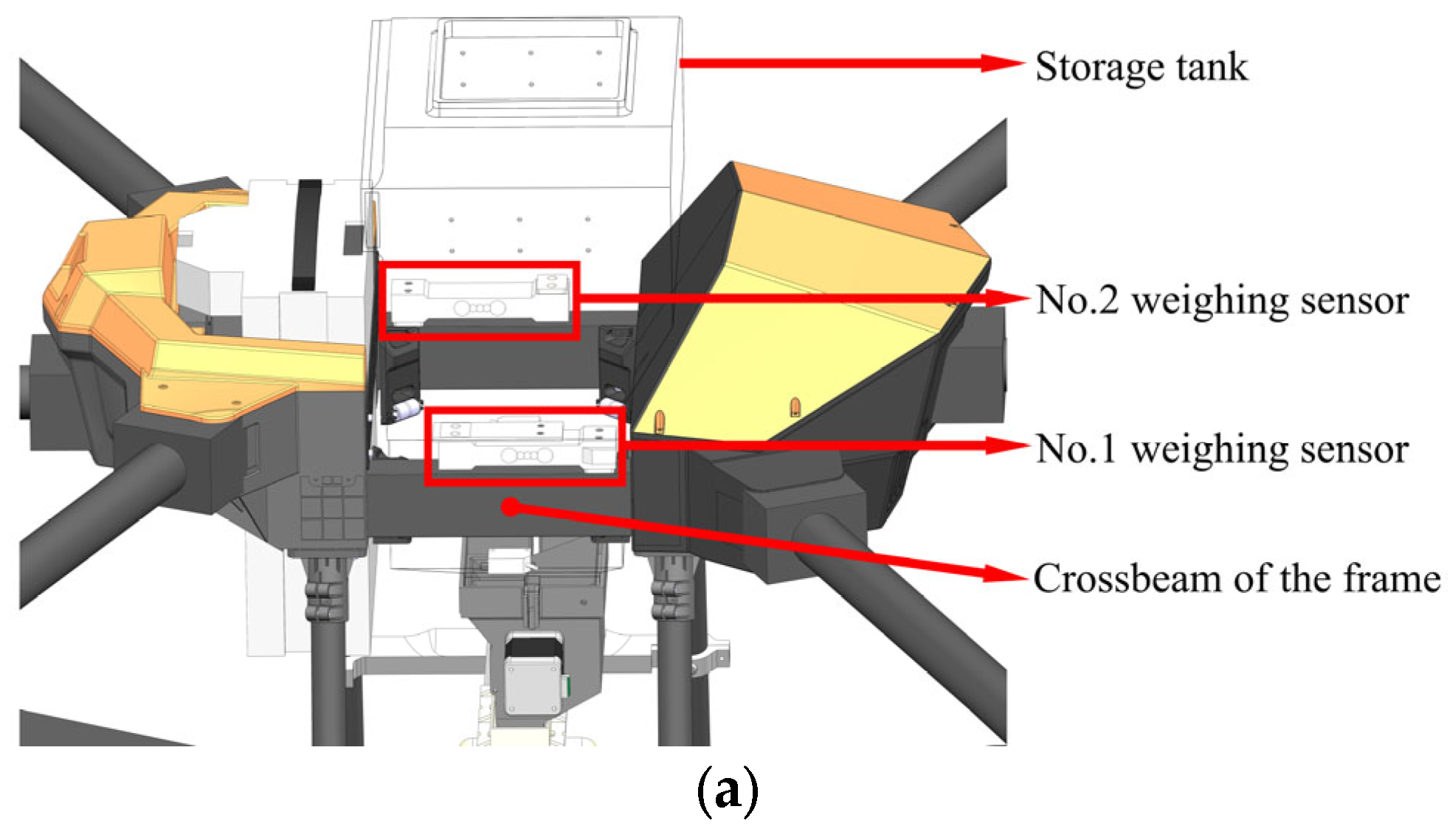
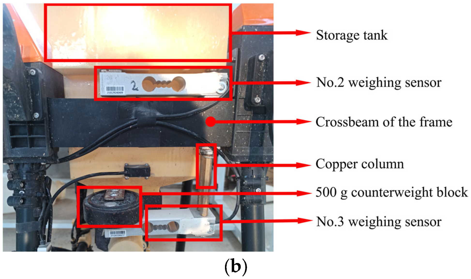
The installation method of the weighing sensor is shown in
Figure 3. Two weighing sensors (No. 1 and No. 2) were used as the main sensors, which were fixed on both sides of the crossbeam of the frame and were used to directly weigh the storage tank. A third weighing sensor (No. 3) was used as a noise monitoring sensor, which was connected to the bottom of the frame beam through a copper column, and the force end of the sensor was fixed to a 500 g counterweight block. When the data processing scheme 1 was adopted, only the data of two main sensors were used; when the data processing scheme 2 was adopted, the data of the two main sensors were used as the reference signal of the LMS adaptive filter, and the data of the noise monitoring sensor were used as the input signal.
2.1.4. Filtering Requirements
The filtering requirements were generally considered from two aspects: convergence speed and convergence accuracy, which sometimes contradict each other, that is, increasing the convergence speed (reducing the convergence time) will lead to a convergence accuracy, and reducing the convergence speed (increasing the convergence time) can improve the convergence accuracy. The specific filtering requirements are as follows:
- (1)
The weight data mentioned in this paper were mainly used to monitor the storage tank and indicate that there was no material left in the storage tank. The quantity monitor is installed on the UAV and connected to the controller of the UAV. During the operation of the UAV, when the quantity monitor detects that there is nothing remaining in the storage tank, it sent an instruction to the UAV’s controller to suspend the operation of the UAV and remind the operator so that the operator can control the UAV to return to the feeding point to add materials, avoiding having the empty storage tank continuing to operate, resulting in missed application. The maximum acceptable error of missed application of the device for the test was 1 m. According to the maximum 3 m/s operating speed of the prototype, the maximum acceptable delay time of the filtered data was 333 ms, that is, the convergence time should be less than 333 ms.
- (2)
When the weighing data were used for the judgment of the shortage warning, if the data fluctuation range is large, the accuracy of the shortage warning will be affected. Therefore, the higher the convergence accuracy is, the better. The average relative error of the weighing data during the UAV flight should be less than 3%.
2.2. Data Preprocessing Based on Butterworth Low-Pass Filter
The main feature of the Butterworth filter is that the frequency response curve in its passband has the maximum flatness. The higher the order of the filter, the better the passband characteristics and flatness [
24]. The Butterworth low-pass filter can be used to reduce the high-frequency vibration noise in the data. The normalized transfer formula of the n-order Butterworth low-pass filter is as follows [
25]:
where
a0,
a1,
a2,
a3, and
an represent polynomial coefficients;
n represents the order of the filter. Although increasing the order of the filter can improve the filtering effect, the delay of the filtered data increases, and the amount of calculation becomes larger. Considering both the delay and computational complexity, a second-order Butterworth low-pass filter is selected to preprocess the data, and its normalized transfer formula is as follows:
Let
, the above transfer formula is discretized by bilinear transformation, and
s can be transformed into
where
fd represents cut-off frequency, and
fs represents sampling frequency. Replacing (3) in (2)
where
b0,
b1,
a1, and
a2 represent coefficients of the filter, and the expression in (5) is the final second-order Butterworth low-pass filter data update formula.
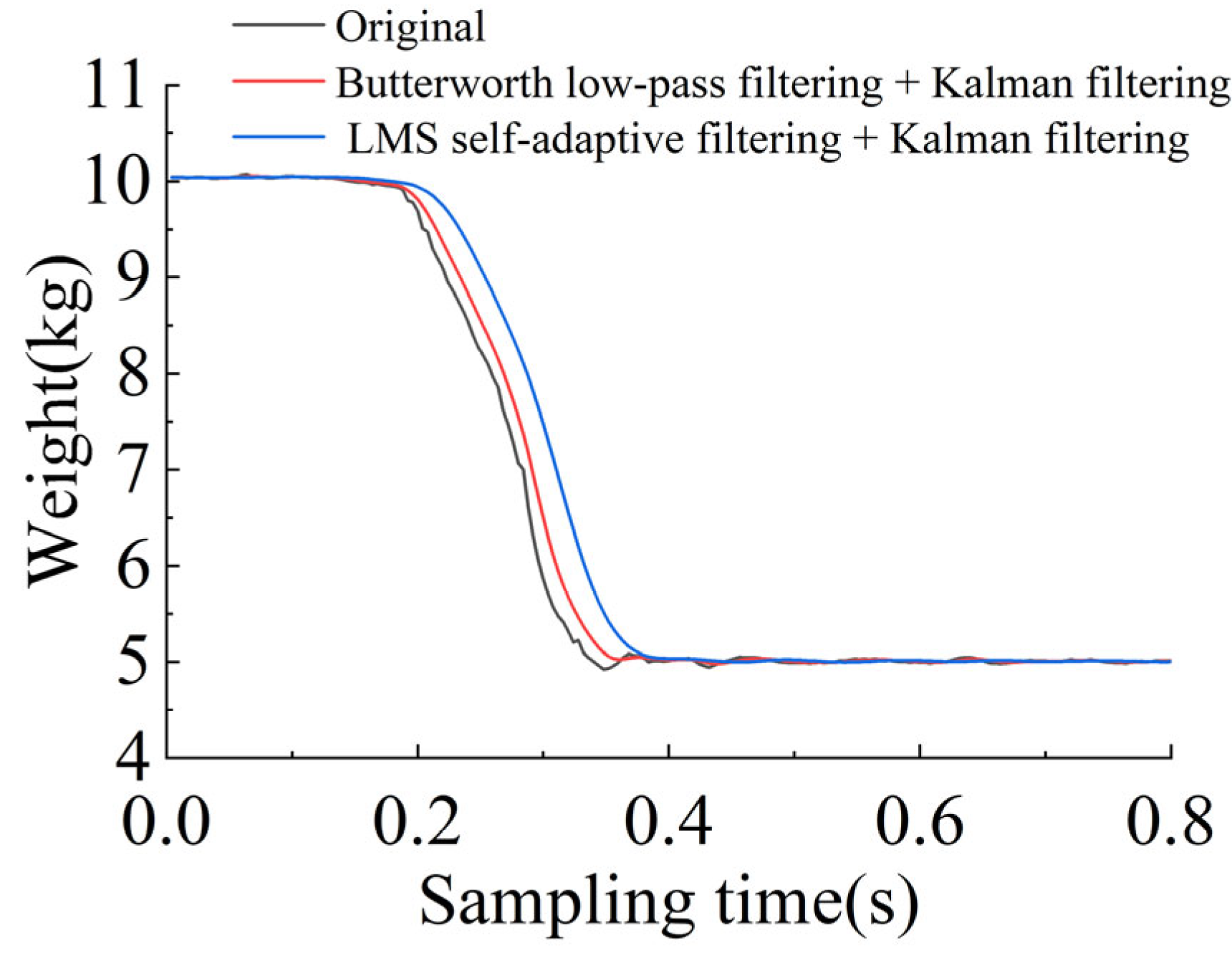
By inputting a step signal to the system, the convergence speed of Butterworth low-pass filter is observed to confirm the cut-off frequency and filter coefficient of the filter. The method was to place 10 kg weight on the storage tank. After the weight data are stable, 5 kg of the weight was reduced in an instant, the data change is observed, and the data are recorded before and after filtering at a sampling frequency of 250 Hz when collecting the data.
2.3. Data Preprocessing Based on LMS Adaptive Filtering
The filter mainly included two parts, namely the Finite Impulse Response (FIR) filter and the coefficient update algorithm. The output signal is generated after the input signal passes through the FIR filter, and the error was calculated after the output signal was compared with the desired signal. The coefficient update algorithm adjusted the coefficients of the FIR filter according to the output signal and the error, so that the error gradually became smaller, and then, the adaptive parameter adjustment and filtering were performed.
The main adjustable parameters of the LMS adaptive filtering algorithm were the order
k and step factor
m. The larger the order, the larger the filter cache, the more data available for the filter reference, but the larger the single calculation; the larger the step size factor, the faster the tracking and convergence speed of the algorithm, but the lower the convergence accuracy. The iterative formula of the LMS adaptive filtering algorithm is [
26]
where
e(
n) is the error at time
n;
d(
n) is the desired signal at time
n;
x(
n) is the input signal at time
n;
y(
n) is the output signal at time
n; and
b(
k) is the k-order filter cache.
The input signal of the LSM adaptive filter is the data of the noise monitoring sensor, the expected signal is the data of the two main sensors, and the output signal is the filtered data. The data of the main sensor will become smaller and smaller due to the continuous reduction of seed weight during UAV working, and the data can be regarded as a signal source containing noise. The weight of the weight block fixed by the noise monitoring sensor is unchanged, but due to the interference of noise, the data will fluctuate continuously, and the data can be regarded as the noise source. After inputting the data of the main sensor and the noise monitoring sensor into the LMS adaptive filter, the coefficient update algorithm constantly adjusts the coefficients of the FIR filter, gradually eliminates the noise of the main sensor data, and makes the output signal gradually approach the real signal source to realize the data filtering.
The step size factor is the main parameter that affects the convergence speed of the LMS adaptive filter. To determine the size of the step size factor, the order of the filter was fixed to 100. By changing the size of the step size factor, the delay time of the data was observed to analyze the convergence speed. The experimental design is as follows:
- (1)
The step size factor was set to 10 levels, ranging from 0.01 to 0.1, and each 0.01 was a level;
- (2)
By inputting the step signal into the system, the convergence speed of the filtering algorithm was observed: 10 kg of weight was placed on the storage tank, and 5 kg of weight was reduced in an instant after the weight data were stable, and the data corresponding to different step-size factors were recorded at a sampling frequency of 250 Hz.
2.4. Data Smoothing
2.4.1. Kalman Filtering
As an optimal estimation algorithm [
27], the Kalman filter algorithm can filter the observation data with noise. In this paper, the linear Kalman filter algorithm was used to further smooth the data. The algorithm mainly includes two parts: prediction and update. The formula is as follows [
28]:
In the above formulas, (11) and (12) are the prediction equations of the algorithm, and (13)–(15) are the update equations of the algorithm. Where represents the predicted state at time k; represents the observation at time k; represents the control effect of the outside world on the system at time k; represents the covariance matrix at time k; represents the prediction noise matrix; represents the measurement noise matrix; represents the Kalman gain at time k; represents the unit matrix; and and represent the corresponding prior variables. When the algorithm is executed, the prior estimation of the state variables is first performed, and the prior covariance is calculated. Then, the Kalman gain is calculated, and finally, the data estimation and covariance update are performed.
When adjusting the parameters of the algorithm, the prediction noise covariance and the observation noise covariance are mainly adjusted. When the increases, the dynamic response becomes faster, that is, the convergence speed is accelerated, but the convergence accuracy is reduced. As increases, the dynamic response becomes slower, that is, the convergence speed becomes slower, but the convergence accuracy is improved. According to the experience of and R tuning parameters, there is a final value of 1.2 and a value of 0.1.
2.4.2. Moving Average Filter
In the actual operation process, the frame of the UAV is prone to random vibration, which causes random noise interference to the weight data. Therefore, it is necessary to further smooth the data. The moving average filtering algorithm has the characteristics of simplicity and small computation and can effectively eliminate the random noise in the data and improve the smoothness of the data. The formula is as follows:
where
y(
n) represents the data after moving average at time
n;
x(
n) represents the input data at time
n; and
L represents the window size of moving average filtering. The window size
L determines the filtering effect of the algorithm. When the algorithm is executed, the moving average is calculated after waiting for
L data. In theory, the data lags
L data. The larger the value of
L, the better the filtering effect, but the longer the data delay time.
In this paper, the convergence time of the expected filtering data is less than 333 ms. After the Kalman filter (in
Section 2.4.1) is added, the convergence time of the two data processing schemes is 260 ms and 280 ms, respectively. Therefore, after the moving average filtering is added in this section, the convergence time can be extended by 73 ms and 53 ms, respectively. The weight data output frequency of this subject is set to 250 Hz (the filtering period is 4 ms), and the window size should be less than 18.25 and 13.25, respectively, so the window size was 18 and 13, respectively.
2.4.3. Static Filtering Effect
The control system designed in this project had the function of seeding quantity calibration, and the weight data needed to be obtained during calibration. The accuracy requirement of the calibration process for the weight data was a deviation of less than 2 g. The static filtering data were analyzed, the data of 10 s were collected, and the accuracy of the data was evaluated by the average deviation. The average deviation calculation method is as follows:
where
E represents the average deviation of the sample (g);
en represents nth filter data (g); and
et represents reference weight (g).
2.5. Data Processing Comparison Test
2.5.1. When the UAV Is Hovering
In the hovering state of the UAV, which means that the UAV is stationary in the air, maintaining a certain height and position, the filtering effects of the two data processing schemes were tested, and the design is as follows:
- (1)
The test was carried out in sunny conditions with a natural wind speed of less than 3 m/s, and the temperature was between 20 and 28 degrees Celsius. The test site was the open space of the wind tunnel laboratory of South China Agricultural University, Guangzhou, China.
- (2)
Before the test, the weight of the storage tank was peeled, and the actual load of the UAV storage tank was changed by adding a 5 kg weight to the storage tank. Five levels of 5, 10, 15, 20, and 25 kg (25 kg is the maximum load) were set up for a total of 5 groups of tests.
- (3)
The hovering height of the UAV was set to 1.5 m. At the same time, two filtering schemes were used to filter the original data in real time, and the update rate (output rate) of the filter was 250 Hz. The data were recorded after the UAV hovered stably, and the data recording time was 30 s, that is, 7500 data points were collected.
The actual weight of 5 bags of heavy objects was recorded before the test. The weight was used as the reference weight in the data analysis. The filtered data were compared with the reference weight, and the data were analyzed from the aspects of maximum deviation, maximum relative error, average relative error, and FFT spectrum. The calculation method of the relative error is as follows:
where
δi represents the relative error of the
i th filtered data (kg);
Xt represents reference weight (kg). The smaller the relative error, the better the filtering effect. The FFT spectrum can reflect the distribution of noise and the size of noise. The smaller the amplitude corresponding to a certain frequency, the smaller the noise in the data corresponding to that frequency.
Six kinds of filter data were recorded during the experiment. To facilitate chart reading and data analysis, the code shown in
Table 3 was used to replace each filter processing.
2.5.2. When the UAV Is Flying
In the actual operation process, the UAV was not only in the hovering state, but also in the switching route state and the flight state. However, the UAV was in the flight state most of the time, so the weight data in the flight state were more important. In this test, the corresponding weight data were analyzed when the prototype was in flight, but its actuator was not working. The specific experimental design is as follows:
- (1)
The test weather conditions and test sites were the same as those in
Section 2.5.1.
- (2)
We planned the route at the ground station to make the prototype fly along the route. The working height was set at 1.5 m, and the working speed was set at three levels of 1, 2, and 3 m/s, respectively. The weight of the storage tank was set to 5 levels, which were 5, 10, 15, 20, and 25 kg (25 kg was the maximum load), and a total of 15 groups of tests were carried out.
- (3)
At the same time, two filtering schemes were used to filter the weight data in real time, and the update rate (output rate) of the filter was 250 Hz. The data were recorded during the flight of the prototype, and the data recording time was 15 s, that is, 3750 data points were collected.
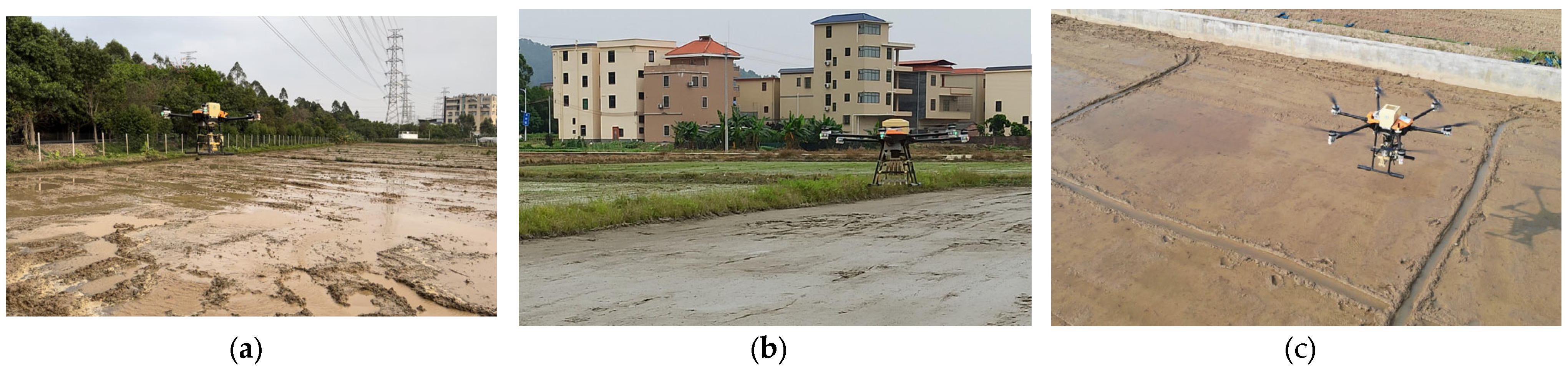
2.6. UAV Seeding Field Test
To further verify the practical application effect of the treatments, three field tests of rice seeding were carried out in the Mark Village, Dongchong Town, Nansha, Guangzhou, China, the Dagang Village, Zhucun Town, Zengcheng, Guangzhou, China, and the Zengcheng Teaching and Research Base of South China Agricultural University, Guangzhou, China. During the test period, the wind speed was less than 3 m/s, and the temperature was between 22 and 30 degrees Celsius. The test sites and planting features are shown in
Figure 4 and
Table 4.
In seeding, it was difficult to obtain reliable reference data because the quantity of the storage tank was becoming smaller and smaller. Therefore, the stability of the monitor for the storage tank mainly performed FFT analysis on the data and observed the noise changes before and after filtering to analyze the stability of the monitor for the storage tank.
The weight data of test 1, test 2, and test 3 were recorded and collected at a frequency of 250 Hz when seeding. After the tests, the weight data of three consecutive routes were selected from each test for comparison and analysis.
4. Discussion
4.1. Analysis of UAV Hovering Test
It can be seen from
Figure 11 that the unfiltered original weight data fluctuate greatly at five load levels. This is due to the vibration of the frame when the UAV was hovering. In addition, the UAV was not kept at the same height, and the UAV continued to move up and down at the target height. The vibration generated by the frame was transmitted to the storage tank, which ultimately caused the measurement result of the weighing sensor to be unstable.
After processing 1 and processing 2, the amplitude of data fluctuation was significantly reduced. Under the load of 5, 10, and 15 kg, the data fluctuation amplitude of treatment 2 was less than that of treatment 1, while under the load of 20 and 25 kg, the data fluctuation amplitude of treatment 1 and treatment 2 was similar, which proves that the filtering effect of treatment 2 was better than that of treatment 1, and the adaptability of treatment 2 was stronger. The reason for this phenomenon may be that under different loads, the vibration of the frame was irregular, and the generated vibration noise was random. Processing 1 set a fixed cut-off frequency, which made it difficult to effectively eliminate random noise. Processing 2 continuously adjusted the coefficient of the filter during execution and had an adaptive adjustment ability, which can better filter out random noise.
After the original data were processed by processing 3 and processing 4, respectively, the amplitude of data fluctuation was further reduced, and the filtering effect was better than that of processing 1 and processing 2, respectively, indicating that the Kalman filter algorithm can effectively reduce the noise and further eliminate the random noise. After the original data were processed by processing 5 and 6, respectively, the amplitude of data fluctuation was further reduced, and the filtering effect was better than that of processing 3 and 4, respectively, which shows that the moving average filtering had a better noise reduction ability and can improve the smoothness of the data.
Table 7 shows that there was a large deviation in the unfiltered data, which was difficult to use directly. After processing 5 and 6, the maximum deviation of the original data was less than 0.5 kg, but under the same load, the maximum deviation of processing 6 was smaller. With the increase in load, the maximum deviation of treatment 5 and treatment 6 became larger, which indicated that the larger the load, the larger the noise generated by the UAV frame and the larger the deviation. From the perspective of maximum relative error, the maximum relative error of the original data after processing 5 was 1.26~2.94%, while the maximum relative error after processing 6 was 1.24~2.74%, indicating that under the same load, the maximum relative error of processing 6 was smaller, so the filtering effect of processing 6 was better. From the perspective of average relative error, the average relative error of the original data was within 1.18~4.80%, the average relative error of treatment 5 was within 0.34~0.66%, and the average relative error of treatment 6 was within 0.31~0.58%, indicating that treatment 5 and treatment 6 had a better filtering effect and met the filtering requirements.
It can be seen from
Figure 12 that a large amount of noise was mixed in the original data. Near the frequencies of 75 and 150 Hz, the fluctuation range of the original data was large, and the noise interference to the data was more serious. After processing 5 and 6, the amplitude corresponding to the same frequency was reduced by about 100 orders of magnitude, and the noise was well suppressed.
4.2. Analysis of UAV Flighting Test
It can be seen from
Figure 13, under the same load, with the increase in working speed, the fluctuation range of data became larger. This is because the greater the speed, the greater the vibration amplitude of the frame, and the greater the noise. At the same operating speed, with the increase in load, the fluctuation range of data became larger, indicating that the noise increases with the increase in load. By comparing the data waveforms of processing 5 and processing 6, it can be seen that the data waveform of processing 5 fluctuates less when the load was 5 and 10 kg, but the fluctuation became larger when the load was 15, 20, and 25 kg, while the data of processing 6 fluctuate slightly near the reference data, which shows that processing 6 encounters larger vibration and noise, better stability, stronger adaptability, and better filtering effect.
In
Table 8, the maximum deviation range of the original data was 1.995~3.666 kg. Overall, the deviation is larger than the original data of the hovering test in
Section 3.4, indicating that the vibration noise of the UAV during flight was larger than that during hovering. With the increase in load and working speed, the maximum deviation of treatment 5 and treatment 6 gradually becomes larger. When the load was 25 kg, the deviation increases obviously. Currently, the maximum deviation of treatment 5 was in the range of 1.064~2.031 kg, and the maximum deviation of treatment 6 is in the range of 0.420~0.888 kg. In contrast, treatment 6 had a better noise suppression ability.
From the perspective of relative error, the maximum relative error of treatment 5 was 4.26~12.84%, and the average relative error was 0.72~2.86%. The maximum relative error of treatment 6 was 1.68~10.06%, and the average relative error was 0.74~2.54%, which all met the filtering requirements. Under the same conditions, the maximum relative error and average relative error of treatment 6 were smaller than those of treatment 5, which shows that treatment 6 has a better noise suppression ability and smoother data filtering data.
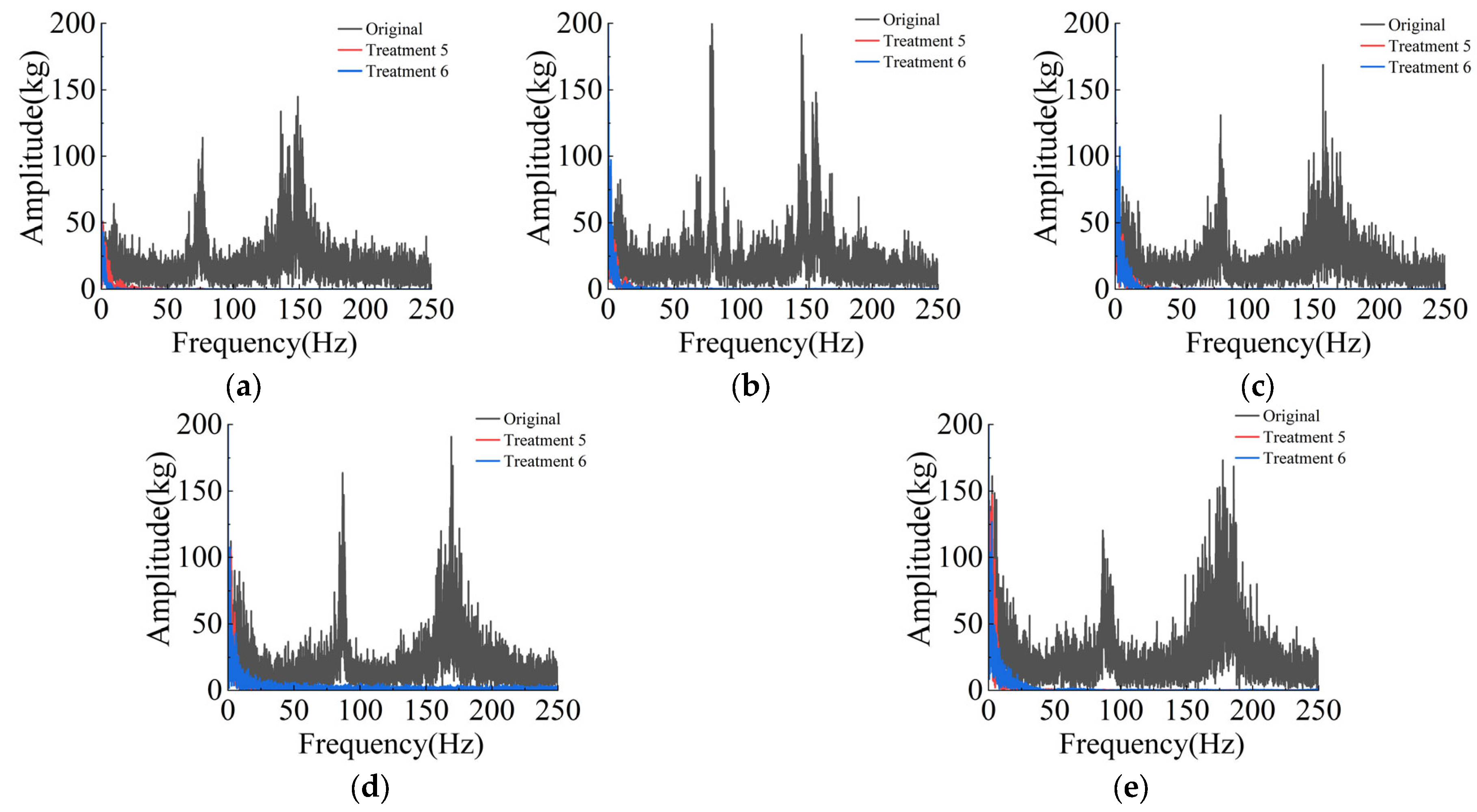
4.3. Analysis of Field Test
Figure 14 shows that the original data are seriously disturbed by the vibration and noise of the UAV, and the data fluctuate in a large range. After processing 2 (LMS adaptive filtering), the stability of the data is greatly improved. After the original data were processed by processing 4 (LMS adaptive filtering + Kalman filtering), the fluctuation range of the data was reduced again, and the noise was further filtered out. After the original data were processed by processing 6 (LKM), the data were smoother, the stability was better, and the noise was effectively suppressed. The data fluctuation range of test 3 was larger than that of test 1 and test 2, because the working speed of test 3 was faster than that of test 1 and test 2. The faster the working speed, the greater the vibration noise and the more unstable the data.
Further analysis shows that when the UAV switches the route, the data had a large fluctuation. The possible reason was that during the switching route, the gravity acceleration of the UAV changed drastically, and the UAV switched continuously in the two states of overweight and weightlessness, resulting in the continuous shaking of the storage tank and the large-scale fluctuation of the data.
The FFT analysis in
Figure 14 shows that the frequency band of noise was widely distributed before filtering, and the noise interference was more serious near the frequency of 75 Hz and 150 Hz. After filtering, the amplitude corresponding to the same frequency was reduced by about 1000 orders of magnitude, and the noise near 75 Hz and 150 Hz was effectively suppressed.
4.4. A Comparison with Existing Research
Obtaining the allowance in the storage tank is very important for various devices in agricultural production and is a key factor in improving the working accuracy of the devices [
29,
30]. In the existing research, the filtering processing of weighing data is often limited to the use of a single filter. This paper innovatively proposes a new processing scheme, that is, multiple filters optimized for different noise types are continuously applied. In order to verify the effectiveness of this scheme, this paper compares several groups of experiments and finds a better filter combination to further improve the accuracy and effect of data processing. Through this continuous filtering method, it can filter out all kinds of noise interference more comprehensively, so as to obtain more accurate and reliable weighing data.
The final filtering scheme adopts the LMS adaptive filtering scheme with fixed step size factor, but the fixed step size factor is difficult to balance with the steady-state error and convergence speed. In order to further improve the filtering effect, the variable-step-size LMS adaptive filtering algorithm can be used in subsequent research [
31]. In addition, compared with existing schemes, a noise monitoring sensor is added to the final determined storage tank allowance monitoring scheme, which means an increase in cost and an increase in installation difficulty. Other schemes can also be tried to further improve the stability and reliability of seed box allowance monitoring data [
32].


 and
and 


