Deep Learning-Based Weed Detection Using UAV Images: A Comparative Study

Abstract

Semantic segmentation has been widely used in precision agriculture, such as weed detection, which is pivotal to increasing crop yields. Various well-established and swiftly evolved AI models have been developed of late for semantic segmentation in weed detection; nevertheless, there is insufficient information about their comparative study for optimal model selection in terms of performance in this field. Identifying such a model helps the agricultural community make the best use of technology. As such, we perform a comparative study of cutting-edge AI deep learning-based segmentation models for weed detection using an RGB image dataset acquired with UAV, called CoFly-WeedDB. For this, we leverage AI segmentation models, ranging from SegNet to DeepLabV3+, combined with five backbone convolutional neural networks (VGG16, ResNet50, DenseNet121, EfficientNetB0 and MobileNetV2). The results show that UNet with EfficientNetB0 as a backbone CNN is the best-performing model compared with the other candidate models used in this study on the CoFly-WeedDB dataset, imparting Precision (88.20%), Recall (88.97%), F1-score (88.24%) and mean Intersection of Union (56.21%). From this study, we suppose that the UNet model combined with EfficientNetB0 could potentially be used by the concerned stakeholders (e.g., farmers, the agricultural industry) to detect weeds more accurately in the field, thereby removing them at the earliest point and increasing crop yields.

1. Introduction

Global food demand is projected to surge by a significant margin of 35% to 56% from 2010 to 2050 [1]. However, the expansion of industrialization, desertification and urbanization has led to a reduction in the crop production area and, hence, productivity of food [2]. In addition to these challenges, climate change is increasingly creating favorable conditions for pests such as insects and weeds, harming crops [3]. Therefore, crop quality and quantity will be affected by insects and weeds if the appropriate treatment is not devised in a timely manner. Traditionally, herbicides and pesticides have been employed as a means of control [4]. When these herbicides are sprayed throughout entire fields without making precise identification of weeds, such an application of herbicides, while serving its purpose, results in a detrimental impact on both crop yield and the environment. While they effectively combat pests and diseases that threaten crops, their use can lead to reduced agricultural productivity due to their excessive use where no weeds are present [5]. Therefore, it is essential to precisely identify the weeds vs. crops, so that cultivated plants can be saved from pesticide harm. As such, there is a requirement for a method of weed management that can gather and assess weed-related data within the agricultural field, while also taking appropriate measures to effectively regulate weed growth on farms [6].

Remote sensing (RS)-based approaches can be an alternative for automated weed detection using satellite imagery [7]. However, the success of satellite-based RS in weed detection is significantly influenced by three major limitations. First, the satellites acquire images with spatial resolutions measured in meters (e.g., Landsat at 30 m and Sentinel at 10 m), which is generally insufficient for analyzing plant- or individual plot-level weed data. Moreover, the fixed schedule of satellite revisits may not align with the timing needed to capture essential crop field images. Additionally, environmental factors like cloud cover frequently hinder the dependable quality of these images.

Recently, the Unmanned Aerial Vehicle (UAV) has made significant progress in its design and capability, including payload flexibility, communication and connectivity, navigation and autonomy, speed and flight time, etc. [8]. It offers versatile revisiting capabilities, allowing farmers/researchers to deploy it when weather conditions permit, ensuring frequent image capture (thus achieving high temporal resolution). Moreover, UAVs can capture images with remarkable spatial detail, closely observing individual plants from an elevated perspective, leading to centimeter-level image resolutions. 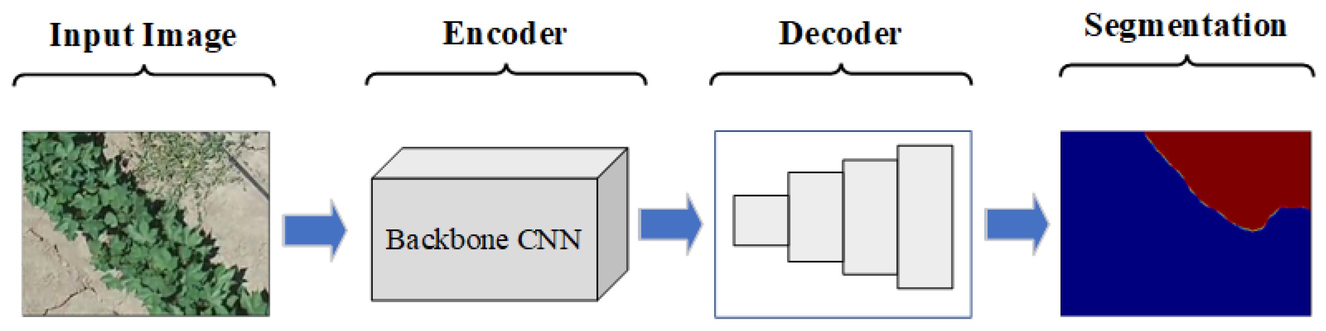Additionally, by flying at lower altitudes, UAVs can bypass cloud cover, obtaining clear and high-quality images [9]. Combined with the high-resolution crop field images acquired with UAV, semantic segmentation methods based on deep learning (DL) can provide a promising method for precise weed detection.

Semantic segmentation (SS) in computer vision is a pixel-level classification task that has revolutionized various fields, such as medical image segmentation [10,11] and precision agriculture (PA) [12]. For instance, Liu et al. [11] utilized the segmentation of retinal images to help diagnose and treat retinal diseases. In the PA domain, SS has been adopted for different problems such as agricultural field boundary segmentation [12], agricultural land segmentation [13], diseased vs. healthy plant detection [14] and weed segmentation [15]. Weed segmentation, which helps to identify unnecessary plants disturbing the growth of crops, is considered one of the major areas that directly contribute to improving crop productivity.

Over recent years, SS has gained significant attraction in the weed detection area of PA. Computer vision techniques that utilize image processing and machine learning methods for weed detection are widely investigated in the literature [16,17,18]. However, deep learning methods for SS have shown state-of-the-art (SOTA) results for image segmentation tasks in general. The availability of pre-trained deep neural networks on large datasets such as ImageNet [19] made it possible to transfer cross-domain knowledge to agriculture field images. For instance, convolutional neural networks (CNNs) such as DeepLab [20], UNet [21] and SegNet [22] are implemented for weed detection on various crop fields. The performance of these neural networks depends on multiple factors, such as the resolution of images, types of crops and field conditions. Since the colour and texture of weeds are very similar to crops, it is a complex problem to make a differentiation between crops and weeds. Furthermore, if more than one type of weed is present in the field, it becomes more challenging to segment such regions.

A few researchers attempted to perform a thorough review and bench-marking of weed detection and segmentation tasks using computer vision and machine learning techniques [23,24]. For instance, Li et al. [23] evaluated the performance of various deep learning methods such as Faster RCNN [25], YOLO [26] and CenterNet [27] for weed detection on publicly available datasets. Additionally, Fathipoor et al. [24] experimented with UNet and its variation for weed segmentation using ground-based RGB images. They achieved an IoU score of 56% with UNet++. Since most of these research works dealt with ground-based RGB images, it is still essential to explore the comparative study of DL methods for weed segmentation using UAV-based RGB images. Despite significant advancements in SS for weed detection, it has the following limitations. First, the existing works lack rigorous comparison to identify the optimal deep learning (DL)-based model for weed segmentation. Second, the performances of these DL-based models are dependent on the use of various CNNs as feature extractors, the number of training images available and the type of regions that need to be segmented or identified. As a result, it might be essential to apply some data augmentation techniques for the effective training of such a DL-based segmentation model when using various backbone CNNs as feature extractors.

Considering the aforementioned limitations, we conduct a detailed comparative study of DL models being used for weed detection and identify the best-performing model in the field. We also evaluate the performance of such SOTA models on a UAV dataset that is publicly available for weed segmentation. In summary, the main contributions of this paper are as follows:

(i)

The comprehensive implementation of five backbone CNNs with three segmentation models for weed detection is achieved. For this, we utilize the patch-based data augmentation method for model building.

(ii)

The performance comparison of five well-established CNNs as feature extractors employed with three segmentation models is reported. For this, we experiment with two strategies: binary segmentation (weed vs. non-weed) and multi-class segmentation (three classes of weed and non-weed).

(iii)

A DL-based method is implemented for weed segmentation using the best-performing backbone CNN and segmentation model.

(iv)

The effect of data augmentation techniques on the learning curve of the DL-based segmentation model while training is compared and reported.

The remainder of the paper is organized as follows: Section 2 presents a literature review, highlighting the summary of the existing works. Section 3 discusses the materials and methods used in this study. Section 4 presents the results and discussion, and Section 5 concludes the paper with future recommendations.

2. Related Work

Owing to the recent advancement in drone and sensor technology, the research on weed detection using DL methods has been swiftly progressing. For instance, a CNN was implemented by Dos et al. [15] for weed detection using aerial images. They acquired soybean (Glycine max) field images in Brazil with a drone and created a database of more than 1500 images including images of the soil, soybeans, broad-leaf and grass weeds. A classification accuracy of 98% was achieved using ConvNet while detecting the broadleaf and grass weeds. However, their approach employed the classification of whole images into different categories for weed detection rather than the segmentation of image pixels into various classes. Similarly, a CNN was implemented for weed mapping in Sod production using aerial images by Zhang et al. [28]. They first processed the UAV images using Pix4DMapper and produced an orthomosaic of the agricultural field. Then, the orthomosaic was divided into smaller image tiles. A CNN was built with an image size of ($125\mathrm{px}\times 125\mathrm{px}$) as input. The CNN achieved a maximum precision of 0.87, 0.82, 0.83, 0.90 and 0.88 for broadleaf, grass weeds, spurge (Euphorbia spp.), sedges (Cyperus spp.) and no weeds, respectively. Ong et al. [29] performed weed detection on a Chinese cabbage field using UAV images. They adapted AlexNet [30] to perform weed detection and compared its performance with traditional machine learning classifiers such as Random forest [31]. The results showed that CNN achieved the highest accuracy of 92.41%, which was 6% higher than that of Random forest. A lightweight deep learning framework for weed detection in soybean fields was implemented by Razfar et al. [32] using MobileNetV2 [33] and ResNet50 [34] networks.

Aside from the single-stage CNNs, few works have been reported that use multi-stage pipelines for weed detection on UAV images. For instance, Bah et al. [35] implemented a three-step method for weed detection on spinach and bean fields using UAV images. First, they detected the crop rows using the Hough transform [36] technique; then, the weeds between these crop rows were used as training samples where a CNN was trained to detect the crop and weed in the UAV images. However, their proposal depends on the accuracy of the line detection technique, which might not be robust when the UAV images contain varying backgrounds and image contrast. A two-stage classifier for weed detection in tobacco crops was implemented in [37]. Here, they first segmented the background pixel from the vegetation pixels which included both weed as well as tobacco pixels. Then, a three-class image segmentation model was implemented. Their proposal achieved the maximum Intersection of Union (IoU) of 0.91 for weed segmentation. However, the two-stage segmentation model requires separate training at each stage, and hence it is not possible to train the model in an end-to-end fashion, adding extra complexity to its deployment.

Object detection approaches such as single shot detector (SSD) [38], Faster RCNN [39] and YOLO [40] were also employed for weed detection using UAV images. For instance, Veeranampalayam et al. [38] compared two object detectors, namely, Faster RCNN and SSD, for weed detection using UAV images. The InceptionV2 [41] model was used for feature extraction in both detectors (Faster RCNN and SSD). The comparison revealed that Faster RCNN models produced a higher accuracy as well as less inference time for weed detection.

The segmentation of images into weed and non-weed regions at the pixel level is more precise and can be beneficial for the accurate application of pesticides. Xu et al. [20] combined the visible color index with a DL-based segmentation model for weed detection in soybean fields. They first generated the visible color index image for each UAV image and fed it into a DL-based segmentation model which utilized the DeeplabV3 [42] network. When comparing its performance with other SOTA segmentation architectures such as fully convolutional neural network (FCNN) [43] and UNet [44], it provided an accuracy of 90.50% and an IoU score of 95.90% for weed segmentation.

3. Materials and Methods

3.1. Dataset

We used a publicly available dataset [45], which consists of 201 RGB images acquired with DJI Phantom Pro 4 from a cotton field in Greece by Krestenitsi et al. [45]. The cotton field images were acquired by flying the UAV at a height of 5 m so that it provides a close clear view of the cotton field. The images were annotated at the pixel level into three types of weeds (Johnson grass (Sorghum halepense), field bindweed (Convolvulus arvensis) and purslane (Portulaca oleracea)) and background.

The dataset includes a total of 201 RGB images of size $1280\mathrm{px}\times 720\mathrm{px}$. In the dataset, there are very few pixels of purslane weeds (only $0.27\times {10}^6$ pixels), whereas the Johnson grass, field bindweed and backgrounds have $1.44\times {10}^6$, $7.56\times {10}^6$ and $175\times {10}^6$ pixels [45], respectively. It is clear that the dataset is highly imbalanced, which make the automated weed detection task more challenging. Sample images and their corresponding mask are shown in Figure 1.

3.2. Patch Generation and Augmentation

Since the images were captured with a drone flying 5 m above the crop, the original image size was 1280 px by 720 px. It is too large to feed into DL models as the large image size requires high memory, thereby slowing the training process [46]. One way of dealing with this is to resize the image while feeding it into the DL model, but this loses the crucial information and the model performance decreases significantly. We employ the patch-based strategy to create small-size patches and use such patches to train the DL models because it has two-fold benefits. First, it increases the training patches, which is essential to train the DL models as they generally contain millions of trainable parameters which require a large number of training samples. Second, it also helps balance the training dataset.

Since the dataset is highly imbalanced (with the majority of the pixels in the background class) and the main focus of this study is weed detection, it is logical to remove the image patches that only include background pixels. Therefore, we set the threshold to remove image patches that include almost all (97%) background pixels (as shown in Figure 2). Following this procedure, each UAV image is divided into patches of size ($256\mathrm{px}\times 256\mathrm{px}$), which results in a total of 786 image patches. This dataset of 786 image patches is divided into train and test sets in a ratio of 8:2 (which results in 628 images for the training set and 158 in the test set).

To see the effect of data augmentation on the performance of DL-based weed segmentation methods, we apply three augmentation techniques, flip (horizontal and vertical), rotation (by 90 degrees) and grid distortion, into each image of the training set. The first transformation is applied with a combination of horizontal flip, random rotation by 90 degrees and grid distortion. The second transformation includes the combination of vertical flip with random rotation and grid [47]. After applying the data augmentation, the training set forms 1884 samples. The detailed statistics of the original (D1) and augmented dataset (D2) are presented in

Table 1. The image patch statistics of two datasets without augmentation (D1) and with augmentation (D2). Note that the images in the test set are not augmented.

Dataset	Augmentation	Train	Test	Total
D1	No	628	158	786
D2	Yes	1884	158	2024

.

3.3. Backbone CNN Models

3.3.1. VGG

VGG [48] is a CNN developed by the Visual Geometry Group (VGG) at Oxford University, which achieved victory in the 2014 ImageNet challenge. It is a large neural network with a layered architecture. It includes an Input layer, Convolution layers, Pooling layers and Dense layers. The number of layers in VGG depends on its depth. It has two variations: VGG16 (sixteen-layer network) and VGG19 (19-layer network). In this work, VGG16 is utilized as a feature extractor which includes 13 Convolution layers, 5 Max-pooling layers and 3 Dense layers.

3.3.2. ResNet

Deep CNNs like VGG16 and VGG19 have shown promising results in large-scale image classification tasks. However, training such models is challenging due to the vanishing gradient problem, where small gradients propagated back through the layers diminish and vanish as the network becomes deeper. To address this issue, researchers introduced skip connections, allowing certain layers to be skipped. These skip connections form residual blocks, which are the core of the ResNet architecture [34], to mitigate the vanishing gradient problem, enabling the training of very deep networks for improved performance in image classification tasks.

The ResNet model offers many variants (based on the depth of the network), such as ResNet18, ResNet34, ResNet50, ResNet101 and so on. In this study, we utilized ResNet50, which comprises 48 Convolution layers, 1 Max-pooling layer and 1 Average pooling layer.

3.3.3. DenseNet

DenseNet [49] is a CNN model that expands on the concept of skip connections seen in ResNet by extending them to multiple steps. The central element of DenseNet is the Dense block, which is used between these connections. In DenseNet, each layer is directly connected to all subsequent layers, creating a dense connectivity pattern. This connectivity ensures that each layer receives input from all preceding layers. Dense blocks consist of Convolution layers with the same feature map size but varying kernel sizes. Based on the specific depth of the network, it has different variations such as DenseNet121, DenseNet169 and DenseNet201. In this study, the DenseNet121 network is utilized, which consists of 120 Convolution layers and 4 Average pooling layers. The DenseNet architecture facilitates robust information flow and feature extraction, making it a valuable tool in various applications.

3.3.4. EfficientNet

CNNs such as ResNet [34] and DenseNet [49] have expanded the network in width, depth and resolution along the different dimensions but not systematically. However, EfficientNet proposed by Tan et al. [50] introduced a methodical strategy for scaling up CNNs using a fixed set of scaling coefficients. The architecture of EfficientNet consists of three main parts: the stem block, the body and the final block. While the stem and final blocks remain consistent across all versions of EfficientNet, the body varies among different versions. The stem block involves several components such as input processing, re-scaling, normalization, padding, convolution, batch normalization and activation layers. On the other hand, the body is composed of five modules, each containing depth-wise convolution, batch normalization and activation layers. In this study, we utilized the smaller version known as EfficientNetB0, which consists of a total of 237 layers excluding the top layer.

3.3.5. MobileNet

MobileNet is a CNN model that utilizes depth-wise convolution [51]. Specifically, MobileNetV2 [33], an improved version of MobileNetV1 [51], introduces additional layers and blocks to enhance its performance. It incorporates one regular Convolution layer, followed by 13 depth-wise separable convolution blocks and another regular Convolution layer. MobileNetV2 also includes an Average pooling layer. Notably, it introduces the Expand layer, Residual connections and Projection layers, along with depth-wise Convolution layers known as Bottleneck residual blocks. These additions contribute to the effectiveness and efficiency of MobileNetV2, making it a powerful architecture for various applications. Here, we utilized MobineNetV2 as a backbone CNN while implementing weed segmentation models.

3.4. DL-Based Segmentation Models

3.4.1. SegNet

SegNet [52] is based on FCNN architecture. It consists of an encoder and decoder followed by a pixel-wise classification layer. The encoder includes convolution and pooling operations to produce sparse feature maps. Then, the decoder up-samples the feature maps using un-pooling operations. The un-pooling operation uses the stored indices from the corresponding encoder pooling layers to precisely locate the feature within the up-sampled map.

In this work, we implement SegNet with various CNNs as feature extractors, as depicted in Figure 3. The corresponding layer used for feature extraction for each CNN is shown in

Table 2. The feature extraction layer for each backbone CNN used in SegNet model.

CNN	Feature Extraction Layer
VGG16	block5_conv3
ResNet	Conv4_block6_out
DenseNet121	pool4_conv
EfficientNet	block5a_expand_activation
MobileNetV2	block_13_expand

. Then, the decoder part of the networks includes the four up-sampling blocks, where the first two blocks consist of one Up-sampling and three Convolution layers and the other two blocks consist of one Up-sampling and two Convolution layers. Finally, the segmentation layer with softmax is implemented.

3.4.2. UNet

UNet [44] consists of two paths, contracting and expansive paths, forming a U-shaped network. It is widely used for image segmentation [13,44]. The contracting path, also known as the encoder down, samples the image by extracting an image feature using a series of convolution and pooling operations. The expansive path, also known as the decoder, up-samples the features and recovers the spatial resolution as to the original images using transposed convolution operations. As an example, the ResNet50-based implementation of UNet is demonstrated in Figure 4. Here, the skip-connection is used from the feature map of each block of the encoder to the corresponding block of the decoder to perform concatenating and up-sampling operations. The feature extraction layers for five backbone CNNs utilized in UNet model are adapted from Kezmann et al. [53].

3.4.3. DeepLabV3+

DeepLab is a state-of-the-art deep learning model for semantic segmentation. It has evolved from DeepLabV1 to the latest DeepLabV3. DeeplabV1 [42] utilized the concept of deep convolutional neural networks (DCNNs) and atrous convolution for semantic segmentation. As atrous convolutions enabled the network to capture the multi-scale contextual information, DeepLabV1 achieved significant results in semantic segmentation tasks. DeepLabV2 further extended DeepLabV1 by introducing the use of atrous spatial pyramid pooling (ASPP) which captures the multi-scale feature at different atrous rates [55]. DeepLabV3 introduced an improved ASPP that utilized global average pooling and various atrous rates to capture contextual information more effectively. It is further enhanced by introducing a decoder module that up-samples the feature maps and combines them with lower level features, as shown in Figure 5. The feature extraction layers for all CNNs used in the DeepLabV3+ segmentation model are also adapted from Kezmann et al. [53].

3.5. Experimental Setup

The experimental setup to conduct the weed segmentation was built on Python-based Keras package [56]. All the experiments were carried out on Google Colab [57] cloud computing platform which utilized an NVIDIA T4 GPU with 12 GB RAM.

For maintaining consistency in comparison, each segmentation model was trained up to maximum epochs of 100, with a learning rate of 0.001 and Adam optimizer. To prevent the over-fitting of the model, an early stopping was implemented with a patient of 10 epochs. The total loss function was calculated from focal loss [58] and dice loss [59]. The Intersection of Union (IoU) score and f-score were used as evaluation functions while training the model. A sample plot of IoU score and loss achieved per epoch while training the UNet model with EfficienetNetB0 as the backbone is reported in Figure 6 (for both D1 and D2 datasets).

The experiments were conducted using two strategies: (a) binary vs. multi-class segmentation and (b) with and without data augmentation. The results of these experiments are reported in Section 4.

3.6. Evaluation Metrics

We utilized five evaluation metrics, namely, Precision (1), Recall (2), F1-score (3), accuracy (4) and the Intersection of Union (IoU) (5) to report the performance of weed segmentation models.

$$P=\frac{T_P}{T_P+F_P}$$

(1)

$$R=\frac{T_P}{T_P+F_N}$$

(2)

$$F1=2\times \frac{P\times R}{P+R}$$

(3)

$$ACC=\frac{T_P+T_N}{T_P+T_N+F_P+F_N}$$

(4)

$$IoU=\frac{T_P}{T_P+F_N+F_P}$$

(5)

where $T_P$, $T_N$, $F_P$ and $F_N$ represent true positive, true negative, false positive and false negative for a given class, respectively.

4. Results and Discussion

4.1. Performance Comparison of Different DL-Based Models for Binary Segmentation

In this section, we present the outcomes of the weed vs. background segmentation task. Since this task exhibits relatively lower complexity, all segmentation models based on DL yielded commendable performance.

The performance of the majority of the models (combination of backbone CNNs plus segmentation models) on both datasets D1 and D2 are similar, which shows that the data augmentation technique has no significant effect on the binary segmentation task (see

Table 3. The segmentation results of three segmentation models with five backbone CNNs for weed vs. background segmentation task. Note that the bold values represent the highest performance.

Backbone CNN	Dataset	Seg. Model	Mean IoU	Precision	Recall	F1-Score	Acc.
VGG16	D1	SegNet	63.50	86.24	85.66	85.92	85.66
		UNet	54.54	85.96	86.23	82.93	86.23
		DeepLabV3+	60.78	84.71	85.40	85.00	85.40
	D2	SegNet	65.38	88.26	85.23	86.20	85.23
		UNet	64.22	87.09	88.06	87.12	87.06
		DeepLabV3+	61.56	85.15	85.92	85.45	85.92
ResNet50	D1	SegNet	65.85	87.46	88.20	87.66	88.20
		UNet	64.67	87.17	87.93	86.74	87.93
		DeepLabV3+	61.33	85.01	85.73	85.30	85.73
	D2	SegNet	63.39	86.06	86.55	86.27	86.55
		UNet	65.57	87.48	88.32	87.63	88.32
		DeepLabV3+	63.57	86.13	86.40	86.26	86.40
DenseNet121	D1	SegNet	67.12	88.25	88.32	88.29	88.32
		UNet	63.18	86.82	87.86	86.71	87.86
		DeepLabV3+	60.25	85.02	86.39	85.20	86.39
	D2	SegNet	67.56	88.26	88.90	88.43	88.90
		UNet	67.13	87.97	88.56	88.17	88.56
		DeepLabV3+	62.35	85.61	85.21	85.40	85.21
EfficientNetB0	D1	SegNet	66.85	87.84	88.44	88.04	88.44
		UNet	66.73	87.85	88.53	88.05	88.53
		DeepLabV3+	58.79	83.88	82.91	83.34	82.91
	D2	SegNet	67.24	87.95	87.88	87.92	87.88
		UNet	66.72	87.82	88.47	88.02	88.47
		DeepLabV3+	61.84	85.53	86.63	85.82	86.63
MobileNetV2	D1	SegNet	65.41	87.14	86.75	86.93	86.75
		UNet	67.07	87.94	87.53	87.71	87.53
		DeepLabV3+	53.85	81.97	84.38	82.08	84.38
	D2	SegNet	64.06	87.52	84.58	85.56	84.58
		UNet	65.42	87.06	87.47	87.24	87.47
		DeepLabV3+	59.87	84.25	85.16	84.61	85.16

). For instance, the highest performing model (DenseNet121 + SegNet) has a mean IoU score of 67.56% on D2 (with augmentation) and 67.12% on D1 (without augmentation). Similar results are seen for other combinations of backbone CNNs and segmentation models (SegNet, UNet and DeepLabV3), except for VGG16. In this case, UNet with VGG16 as a backbone improves its mean IoU score of 54.54% to 64.22% when the data augmentation technique is utilized.

Upon evaluating the backbone CNNs without employing augmentation (D1), both ResNet50 and DenseNet121 yield a mean IoU score exceeding 60% across all three segmentation models (SegNet, UNet and DeepLabV3+). Among these three segmentation models, SegNet achieves the highest mean IoU score of 67.12% when paired with DenseNet121. It also demonstrates competitive results with a mean IoU score of 66.85% for EfficientNetB0, 65.85% for ResNet50 and 63.50% for VGG16, except for MobileNetV2. In this case, UNet outperforms all other models, attaining a mean IoU score of 67.07%. Comparing the results of backbone CNNs on the augmented dataset (D2), DenseNet121 and EfficientNetB0 produce the highest mean IoU score of 67.56% and 67.24% when combined with the SegNet model, respectively, whereas MobineNetV2 with UNet shows a competitive performance (mean IoU score of 67.07%).

Regarding accuracy comparison, the SegNet model with both DenseNet121 and EfficintNetBO as backbones achieves the highest accuracy, surpassing 88%. Notably, the DeepLabV3+ model with VGG16 as its backbone displays the lowest performance. This disparity in performance might be attributed to the limited availability of training data for the models.

4.2. Comparative Study of DL-Based Models for Multi-Class Segmentation

The results of the multi-class segmentation task are discussed. Since this task aims to segment the image region into four classes, including three types of weed and background, it is really challenging to distinguish each pixel from one class to another class for most of the segmentation models. Distinguishing the weed classes is considerably complex due to the resemblances in texture, color and patterns exhibited by distinct types of weeds. This similarity substantially contributes to the challenges encountered in effectively categorizing these diverse weed species.

For the multi-class task, the performance of the majority of the models is increased with data augmentation. For instance, EfficientNetB0 combined with UNet produces a mean IoU of 56.21%, whereas its mean IoU is only 51.97% when data augmentation is not applied (see

Table 4. The segmentation results of three segmentation models with five backbone CNNs for multi-class segmentation task. Note that the bold values represent the highest performance.

Backbone CNN	Dataset	Seg. Model	Mean IoU	Precision	Recall	F1-Score	Acc.
VGG16	D1	SegNet	54.41	87.62	87.32	87.41	87.32
		UNet	44.30	81.98	84.54	82.20	84.54
		DeepLabV3+	42.16	84.77	83.66	84.01	83.66
	D2	SegNet	43.72	83.29	85.24	81.79	85.24
		UNet	51.71	86.13	86.36	86.12	86.36
		DeepLabV3+	41.35	85.34	85.62	85.19	85.62
ResNet50	D1	SegNet	51.64	86.92	87.82	87.01	87.82
		UNet	53.30	86.55	87.37	86.77	87.37
		DeepLabV3+	42.43	85.13	82.93	83.72	82.93
	D2	SegNet	53.24	86.58	85.93	86.17	85.93
		UNet	56.09	87.80	87.67	87.70	87.67
		DeepLabV3+	48.34	86.06	85.68	85.75	85.68
DenseNet121	D1	SegNet	52.18	87.91	88.22	88.03	88.22
		UNet	53.94	87.31	88.26	87.37	88.26
		DeepLabV3+	40.32	85.20	84.42	84.48	84.42
	D2	SegNet	52.06	86.75	87.69	86.95	87.69
		UNet	56.04	88.19	88.16	88.11	88.16
		DeepLabV3+	40.94	85.42	84.89	84.95	84.89
EfficientNetB0	D1	SegNet	51.84	86.87	86.01	86.29	86.01
		UNet	51.97	87.51	88.26	87.63	88.26
		DeepLabV3+	39.86	83.86	82.85	83.16	82.85
	D2	SegNet	53.30	85.68	86.66	85.98	86.66
		UNet	56.21	88.20	88.97	88.24	88.97
		DeepLabV3+	40.74	84.46	85.94	84.60	85.94
MobileNetV2	D1	SegNet	47.90	86.82	86.63	86.60	86.63
		UNet	44.49	86.20	87.30	85.42	87.30
		DeepLabV3+	33.06	82.33	80.44	81.17	80.44
	D2	SegNet	47.00	86.38	87.54	86.39	87.54
		UNet	55.77	87.48	88.37	87.59	88.37
		DeepLabV3+	32.56	83.82	83.82	83.30	83.82

).

Among the three segmentation models, UNet with EfficientNetB0 produces the highest mean IoU of 56.21%. It is noted that UNet performed well with other backbone CNNs as compared with SegNet and DeepLabV3+. For instance, the mean IoU of UNet with DenseNet121 is 56.09%, which is the second-highest performance among the compared models.

Comparing the performance of five backbone CNNs, ResNet50, DenseNet121 and EfficientNetB0 achieve a mean IoU score of above 50% when combined with UNet and SegNet on both datasets (D1 and D2). MobileNetV2 combined with DeepLabV3+ has a mean IoU of 32.56% for D1 and 33.06% for D2.

It is observed that DenseNet121 with SegNet performs the best for the binary task, whereas EfficieentNetBo with UNet achieves the best performance for the multi-class task. However, the combination of other backbone CNN and segmentation models also yields a similar performance for the binary task. It might be attributed to the relatively lower complexity associated with the binary segmentation problem, where all models are able to discriminate between the background (also includes the crops) and weeds. In comparison, the multi-class segmentation task is more challenging as it has higher intra-classes similarity between the different types of weeds. Since UNet [4] transfers the entire feature from encoder to decoder, they might help discriminate the multiple weed classes for multi-class segmentation. This is further supported by the consistently higher performance of UNet in the majority of backbone CNNs for the multi-class segmentation task (refer to Table 4).

The pixel-wise classification accuracy of most of the models ranges from 75% to 88%, which shows that the DL-based segmentation models are able to learn some patterns from the UAV images and have some potential in weed segmentation.

4.3. Class-Wise Study of Best-Performing DL-Based Segmentation Model

We report the class-wise performance of the best models; DenseNet121 with SegNet for the binary and EfficientNetB0 with UNet for the multi-class segmentation.

Table 5. Class-wise performance of SegNet with DenseNet121 as backbone CNN for weed vs. background segmentation. Note that the performance metrics are reported in percentages (%).

Class	IoU	Precision	Recall	F1-Score
Background	87.66	91.68	95.24	93.42
Weed	47.46	71.78	58.36	64.37

shows that the model is able to identify the background class with all the performance matrices ( IoU of 87.66%, precision 91.68%, Recall 95.24% and F1-score 96.42) higher than 87%. However, the performance metrics for the weed class ranged from 47% (IoU) to 71% (Precision).

For the multi-class segmentation, the background class has the highest performance (IoU of 88.09%), while the weed class (Johnson grass) has the lowest performance (IoU of 44.78%) (refer to

Table 6. Class-wise performance of UNet with EfficientNetB0 as backbone CNN for multi-class segmentation. Note that the performance metrics are reported in percentages (%).

Class	IoU	Precision	Recall	F1-Score
Background	88.09	91.12	96.26	93.62
Johnson grass	44.78	79.04	50.82	63.70
Bind weed	46.73	82.00	52.08	63.70
Purslane	45.31	72.94	54.47	62.37

). It seems that it is more challenging to distinguish between the types of weeds than to differentiate between background vs. weed pixels.

4.4. Five-Fold Results of Best-Performing Model

To perform the validation of the best-performing model, we provide the five-fold cross-validation results for the multi-class (EfficientNetB0+UNet)) segmentation model. The confidence interval (CI) (refer to Equation (6)) for each performance metric is calculated at a 95% confidence level, which shows the statistical estimate of performance among the five folds of the dataset [60].

$$CI=\mu \pm z\frac{\sigma }{\sqrt{n}}$$

(6)

where $\mu ,z,\sigma$ and n represent the sample mean, confidence level, sample standard deviation and sample size. We preferred the CI over the p-value in this statitical analysis because the interpretation of trial results based solely on p-values can be misleading [61].

Table 7. Five-fold results for multi-class segmentation task (EfficientNet + UNet) with data augmentation (D2). Note that the CI represents the confidence interval at $\alpha =0.05$.

Fold	Mean IoU	Precision	Recall	F1-Score
Fold-1	58.05	87.82	88.09	87.88
Fold-2	57.17	87.93	88.28	88.00
Fold-3	60.43	87.65	88.25	87.88
Fold-4	56.21	88.20	88.97	88.24
Fold-5	57.17	87.48	87.93	87.67
CI	$57.80\pm 1.4$	$87.81\pm 0.24$	$88.304\pm 0.34$	$87.93\pm 0.18$

reports the performance scores of the EfficientNetB0 with UNet model for five folds, shedding light on the consistency of the model across the folds. The performance of the model in Fold-3 (mean IoU of 60.43%) is the highest, followed by the Fold-1 (mean IoU of 58.05%). The minimum scores of the models are reported in Fold-4 (mean IoU of 56.21%). However, the confidence interval (CI) at $\alpha =0.05$ shows that the model is robust across the fold with the minimum margin of errors ($\pm 1.4\%$ for IoU, $\pm 0.24\%$ for precision, $\pm 0.34\%$ for recall and $\pm 0.18\%$ for f-score) from the mean.

4.5. A DL-Based Framework for Weed Detection on UAV Images

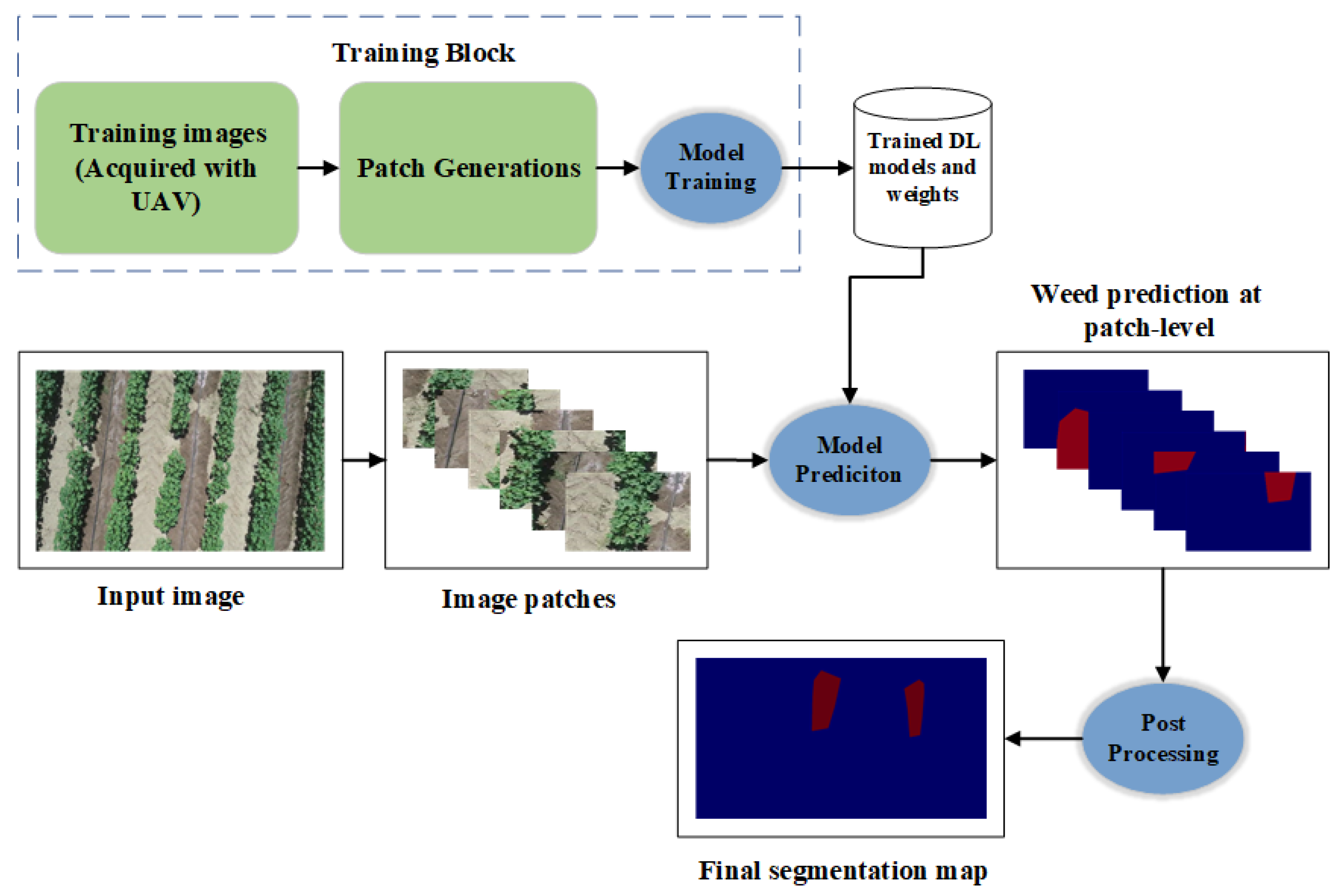
We finally present the DL-based framework for weed detection using UAV images, which consists of five stages: (a) input UAV-acquired images, (b) patch generations, (c) load the trained DL model at patch level, (d) make the prediction, (e) post-process the patch level prediction and (f) generate the final segmentation map (refer to Figure 7).

The framework begins with large input images (($1570\mathrm{px}\times 720\mathrm{px}$)), and the image is divided into smaller patches of size ($256\mathrm{px}\times 256\mathrm{px}$). By dividing the whole image into manageable patches, we believe that the backbone CNNs can focus on discriminating features within localized areas that include weed pixels. Then, the best-performing DL-based segmentation model (e.g., EfficientNetB0 with UNet) is loaded and deployed to make the segmentation mask prediction at the patch level. The model evaluates the content of each patch and predicts types of weeds and background pixels based on the knowledge acquired during training (binary or multi-class). Finally, after obtaining predictions for individual patches, the framework proceeds to post-process these predictions. This step involves refining and combining the patch-level predictions to generate a more coherent and accurate prediction map for the whole image. In order to deploy the proposed DL framework for weed segmentation for new crop fields (other crops and weed types), the steps included in the training block (see Figure 7) are required, which will train the model to learn how to discriminate the specific crops vs. weeds. The trained model can then be deployed to predict the weeds in the given field image.

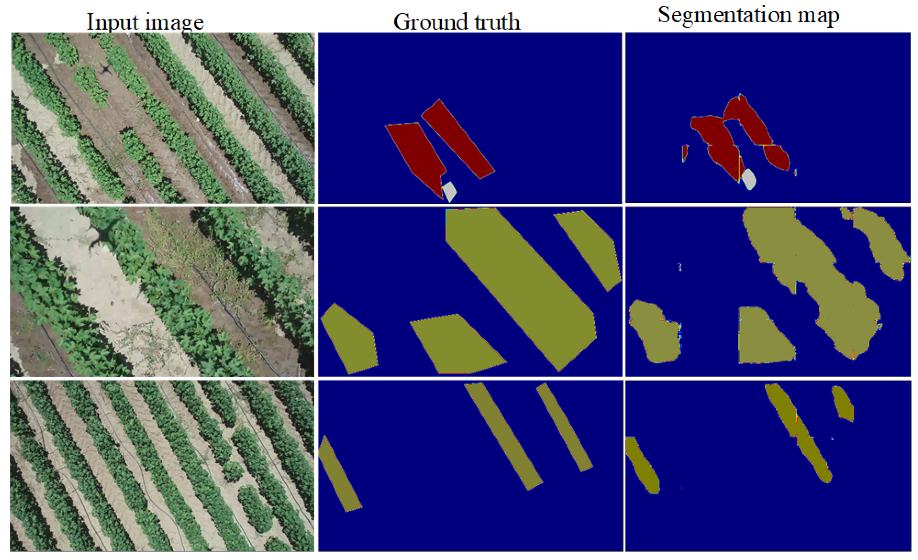
By applying the above procedure, we tested the efficacy of the proposed framework (using EfficientNetB0 with UNet) for a multi-class segmentation task. The sample output generated by the proposed framework is demonstrated in Figure 8.

5. Conclusions

In this work, we comprehensively studied the well-established deep learning-based segmentation models for weed detection. Through the investigation of weed segmentation using UAV images in three aspects, backbone CNNs, segmentation models and data augmentation, binary as well as multi-class weed segmentation frameworks are suggested. The results indicate that DenseNet121 paired with SegNet performs the best for the binary task, while EfficientNetB0 combined with UNet poses the highest performance for multi-class segmentation. Furthermore, the comparison of five backbone CNNs on the benchmark dataset shows that the UNet model with the EfficienNet, DensNet121 and ResNet50 backbone has the best performance on multi-class weed detection. The other models have varying results while using different CNNs as the backbone.

Comparing the three segmentation models (UNet, SegNet and DeepLabV3+) with different backbones, we find a mixed performance on both binary and multi-class segmentation tasks. In particular, in the binary task, SegNet (with DenseNet121 as backbone CNN) has the highest mean IoU score of 67.56%, whereas UNet (with EfficientNetBO) has the highest mean IoU score for multi-class segmentation tasks.

Based on the complexity of segmentation tasks (binary and multi-class), the majority of models (combination of backbone CNNs and segmentation models) demonstrate similar performance for the binary task. This similarity might be attributed to the relatively lower complexity of binary segmentation, where all models effectively distinguish between the background (including crops) and weeds. In contrast, the multi-class segmentation task is more challenging due to higher intra-class similarity between different types of weeds, where UNet excels compared with the other models, which might be attributed to its ability to transfer the entire feature from encoder to decoder during segmentation.

This work has two limitations. First, the model is trained with RGB images which only include the visible light spectrum. Multispectral images can capture more canopy information and might be helpful in learning distinguishable patterns between the weeds and the background. This might further boost the performance of the segmentation models, as these SOTA models have shown the greatest performance in other domains. Second, the effect of data augmentation on multi-class task performance in most of the models indicates the necessity of more training data for improved performance. Data generation techniques such as generative models can be employed to increase the dataset.

References

1. Van Dijk, M.; Morley, T.; Rau, M.L.; Saghai, Y. A meta-analysis of projected global food demand and population at risk of hunger for the period 2010–2050. Nat. Food 2021, 2, 494–501. [Google Scholar] [CrossRef] [PubMed]
2. Satterthwaite, D.; McGranahan, G.; Tacoli, C. Urbanization and its implications for food and farming. Philos. Trans. R. Soc. B Biol. Sci. 2010, 365, 2809–2820. [Google Scholar] [CrossRef] [PubMed]
3. Oerke, E.C. Crop losses to pests. J. Agric. Sci. 2006, 144, 31–43. [Google Scholar] [CrossRef]
4. Huang, H.; Lan, Y.; Deng, J.; Yang, A.; Deng, X.; Zhang, L.; Wen, S. A semantic labeling approach for accurate weed mapping of high resolution UAV imagery. Sensors 2018, 18, 2113. [Google Scholar] [CrossRef] [PubMed]
5. Molina-Villa, M.A.; Solaque-Guzmán, L.E. Machine vision system for weed detection using image filtering in vegetables crops. Rev. Fac. Ing. Univ. Antioq. 2016, 80, 124–130. [Google Scholar]
6. Ofosu, R.; Agyemang, E.D.; Márton, A.; Pásztor, G.; Taller, J.; Kazinczi, G. Herbicide Resistance: Managing Weeds in a Changing World. Agronomy 2023, 13, 1595. [Google Scholar] [CrossRef]
7. Shendryk, Y.; Rossiter-Rachor, N.A.; Setterfield, S.A.; Levick, S.R. Leveraging high-resolution satellite imagery and gradient boosting for invasive weed mapping. IEEE J. Sel. Top. Appl. Earth Obs. Remote Sens. 2020, 13, 4443–4450. [Google Scholar] [CrossRef]
8. Mohsan, S.A.H.; Othman, N.Q.H.; Li, Y.; Alsharif, M.H.; Khan, M.A. Unmanned aerial vehicles (UAVs): Practical aspects, applications, open challenges, security issues, and future trends. Intell. Serv. Robot. 2023, 16, 109–137. [Google Scholar] [CrossRef]
9. Luna, I.; Lobo, A. Mapping crop planting quality in sugarcane from UAV imagery: A pilot study in Nicaragua. Remote Sens. 2016, 8, 500. [Google Scholar] [CrossRef]
10. Ryu, J.; Rehman, M.U.; Nizami, I.F.; Chong, K.T. SegR-Net: A deep learning framework with multi-scale feature fusion for robust retinal vessel segmentation. Comput. Biol. Med. 2023, 163, 107132. [Google Scholar] [CrossRef]
11. Liu, H.; Huo, G.; Li, Q.; Guan, X.; Tseng, M.L. Multiscale lightweight 3D segmentation algorithm with attention mechanism: Brain tumor image segmentation. Expert Syst. Appl. 2023, 214, 119166. [Google Scholar] [CrossRef]
12. Waldner, F.; Diakogiannis, F.I. Deep learning on edge: Extracting field boundaries from satellite images with a convolutional neural network. Remote Sens. Environ. 2020, 245, 111741. [Google Scholar] [CrossRef]
13. Safarov, F.; Temurbek, K.; Jamoljon, D.; Temur, O.; Chedjou, J.C.; Abdusalomov, A.B.; Cho, Y.I. Improved Agricultural Field Segmentation in Satellite Imagery Using TL-ResUNet Architecture. Sensors 2022, 22, 9784. [Google Scholar] [CrossRef] [PubMed]
14. Shahi, T.B.; Xu, C.Y.; Neupane, A.; Guo, W. Recent Advances in Crop Disease Detection Using UAV and Deep Learning Techniques. Remote Sens. 2023, 15, 2450. [Google Scholar] [CrossRef]
15. dos Santos Ferreira, A.; Freitas, D.M.; da Silva, G.G.; Pistori, H.; Folhes, M.T. Weed detection in soybean crops using ConvNets. Comput. Electron. Agric. 2017, 143, 314–324. [Google Scholar] [CrossRef]
16. Al-Badri, A.H.; Ismail, N.A.; Al-Dulaimi, K.; Salman, G.A.; Khan, A.; Al-Sabaawi, A.; Salam, M.S.H. Classification of weed using machine learning techniques: A review—challenges, current and future potential techniques. J. Plant Dis. Prot. 2022, 129, 745–768. [Google Scholar] [CrossRef]
17. Tellaeche, A.; Pajares, G.; Burgos-Artizzu, X.P.; Ribeiro, A. A computer vision approach for weeds identification through Support Vector Machines. Appl. Soft Comput. 2011, 11, 908–915. [Google Scholar] [CrossRef]
18. Wu, Z.; Chen, Y.; Zhao, B.; Kang, X.; Ding, Y. Review of weed detection methods based on computer vision. Sensors 2021, 21, 3647. [Google Scholar] [CrossRef]
19. Deng, J.; Dong, W.; Socher, R.; Li, L.J.; Li, K.; Fei-Fei, L. Imagenet: A large-scale hierarchical image database. In Proceedings of the 2009 IEEE Conference on Computer Vision and Pattern Recognition, IEEE, Miami, FL, USA, 20–25 June 2009; pp. 248–255. [Google Scholar]
20. Xu, B.; Fan, J.; Chao, J.; Arsenijevic, N.; Werle, R.; Zhang, Z. Instance segmentation method for weed detection using UAV imagery in soybean fields. Comput. Electron. Agric. 2023, 211, 107994. [Google Scholar] [CrossRef]
21. Genze, N.; Ajekwe, R.; Güreli, Z.; Haselbeck, F.; Grieb, M.; Grimm, D.G. Deep learning-based early weed segmentation using motion blurred UAV images of sorghum fields. Comput. Electron. Agric. 2022, 202, 107388. [Google Scholar] [CrossRef]
22. Ma, X.; Deng, X.; Qi, L.; Jiang, Y.; Li, H.; Wang, Y.; Xing, X. Fully convolutional network for rice seedling and weed image segmentation at the seedling stage in paddy fields. PLoS ONE 2019, 14, e0215676. [Google Scholar] [CrossRef]
23. Li, Y.; Guo, Z.; Shuang, F.; Zhang, M.; Li, X. Key technologies of machine vision for weeding robots: A review and benchmark. Comput. Electron. Agric. 2022, 196, 106880. [Google Scholar] [CrossRef]
24. Fathipoor, H.; Shah-Hosseini, R.; Arefi, H. Crop and Weed Segmentation on Ground-Based Images Using Deep Convolutional Neural Network. ISPRS Ann. Photogramm. Remote Sens. Spat. Inf. Sci. 2023, 10, 195–200. [Google Scholar] [CrossRef]
25. Saleem, M.H.; Potgieter, J.; Arif, K.M. Weed detection by faster RCNN model: An enhanced anchor box approach. Agronomy 2022, 12, 1580. [Google Scholar] [CrossRef]
26. Dang, F.; Chen, D.; Lu, Y.; Li, Z. YOLOWeeds: A novel benchmark of YOLO object detectors for multi-class weed detection in cotton production systems. Comput. Electron. Agric. 2023, 205, 107655. [Google Scholar] [CrossRef]
27. Jin, X.; Che, J.; Chen, Y. Weed identification using deep learning and image processing in vegetable plantation. IEEE Access 2021, 9, 10940–10950. [Google Scholar] [CrossRef]
28. Zhang, J.; Maleski, J.; Jespersen, D.; Waltz Jr, F.; Rains, G.; Schwartz, B. Unmanned Aerial System-Based Weed Mapping in Sod Production Using a Convolutional Neural Network. Front. Plant Sci. 2021, 12, 702626. [Google Scholar] [CrossRef] [PubMed]
29. Ong, P.; Teo, K.S.; Sia, C.K. UAV-based weed detection in Chinese cabbage using deep learning. Smart Agric. Technol. 2023, 4, 100181. [Google Scholar] [CrossRef]
30. Krizhevsky, A.; Sutskever, I.; Hinton, G.E. Imagenet classification with deep convolutional neural networks. Adv. Neural Inf. Process. Syst. 2012, 25, 1–9. [Google Scholar] [CrossRef]
31. Shahi, T.B.; Xu, C.Y.; Neupane, A.; Fleischfresser, D.B.; O’Connor, D.J.; Wright, G.C.; Guo, W. Peanut yield prediction with UAV multispectral imagery using a cooperative machine learning approach. Electron. Res. Arch. 2023, 31, 3343–3361. [Google Scholar] [CrossRef]
32. Razfar, N.; True, J.; Bassiouny, R.; Venkatesh, V.; Kashef, R. Weed detection in soybean crops using custom lightweight deep learning models. J. Agric. Food Res. 2022, 8, 100308. [Google Scholar] [CrossRef]
33. Sandler, M.; Howard, A.; Zhu, M.; Zhmoginov, A.; Chen, L.C. Mobilenetv2: Inverted residuals and linear bottlenecks. In Proceedings of the IEEE Conference on Computer Vision and Pattern Recognition, Salt Lake City, UT, USA, 18–23 June 2018; pp. 4510–4520. [Google Scholar]
34. He, K.; Zhang, X.; Ren, S.; Sun, J. Deep residual learning for image recognition. In Proceedings of the IEEE Conference on Computer Vision and Pattern Recognition, Las Vegas, NV, USA, 26 June–1 July 2016; pp. 770–778. [Google Scholar]
35. Bah, M.D.; Hafiane, A.; Canals, R. Deep learning with unsupervised data labeling for weed detection in line crops in UAV images. Remote Sens. 2018, 10, 1690. [Google Scholar] [CrossRef]
36. Mukhopadhyay, P.; Chaudhuri, B.B. A survey of Hough Transform. Pattern Recognit. 2015, 48, 993–1010. [Google Scholar] [CrossRef]
37. Moazzam, S.I.; Khan, U.S.; Qureshi, W.S.; Nawaz, T.; Kunwar, F. Towards automated weed detection through two-stage semantic segmentation of tobacco and weed pixels in aerial Imagery. Smart Agric. Technol. 2023, 4, 100142. [Google Scholar] [CrossRef]
38. Veeranampalayam Sivakumar, A.N.; Li, J.; Scott, S.; Psota, E.; J. Jhala, A.; Luck, J.D.; Shi, Y. Comparison of object detection and patch-based classification deep learning models on mid-to late-season weed detection in UAV imagery. Remote Sens. 2020, 12, 2136. [Google Scholar] [CrossRef]
39. Ajayi, O.G.; Ashi, J. Effect of varying training epochs of a Faster Region-Based Convolutional Neural Network on the Accuracy of an Automatic Weed Classification Scheme. Smart Agric. Technol. 2023, 3, 100128. [Google Scholar] [CrossRef]
40. Gallo, I.; Rehman, A.U.; Dehkordi, R.H.; Landro, N.; La Grassa, R.; Boschetti, M. Deep object detection of crop weeds: Performance of YOLOv7 on a real case dataset from UAV images. Remote Sens. 2023, 15, 539. [Google Scholar] [CrossRef]
41. Szegedy, C.; Vanhoucke, V.; Ioffe, S.; Shlens, J.; Wojna, Z. Rethinking the inception architecture for computer vision. In Proceedings of the IEEE Conference on Computer Vision and Pattern Recognition, Las Vegas, NV, USA, 27–30 June 2016; pp. 2818–2826. [Google Scholar]
42. Chen, L.C.; Papandreou, G.; Kokkinos, I.; Murphy, K.; Yuille, A.L. Semantic image segmentation with deep convolutional nets and fully connected CRFs. arXiv 2014, arXiv:1412.7062. [Google Scholar]
43. Long, J.; Shelhamer, E.; Darrell, T. Fully convolutional networks for semantic segmentation. In Proceedings of the IEEE Conference on Computer Vision and Pattern Recognition, Boston, MA, USA, 7–12 June 2015; pp. 3431–3440. [Google Scholar]
44. Ronneberger, O.; Fischer, P.; Brox, T. U-net: Convolutional networks for biomedical image segmentation. In Proceedings of the Medical Image Computing and Computer-Assisted Intervention–MICCAI 2015: 18th International Conference, Munich, Germany, 5–9 October 2015; Proceedings, Part III 18. Springer: Berlin/Heidelberg, Germany, 2015; pp. 234–241. [Google Scholar]
45. Krestenitis, M.; Raptis, E.K.; Kapoutsis, A.C.; Ioannidis, K.; Kosmatopoulos, E.B.; Vrochidis, S.; Kompatsiaris, I. CoFly-WeedDB: A UAV image dataset for weed detection and species identification. Data Brief 2022, 45, 108575. [Google Scholar] [CrossRef]
46. Tan, M.; Le, Q. Efficientnetv2: Smaller models and faster training. In Proceedings of the International Conference on Machine Learning, PMLR, Virtual, 18–24 July 2021; pp. 10096–10106. [Google Scholar]
47. Buslaev, A.; Iglovikov, V.I.; Khvedchenya, E.; Parinov, A.; Druzhinin, M.; Kalinin, A.A. Albumentations: Fast and Flexible Image Augmentations. Information 2020, 11, 125. [Google Scholar] [CrossRef]
48. Simonyan, K.; Zisserman, A. Very Deep Convolutional Networks for Large-Scale Image Recognition. In Proceedings of the International Conference on Learning Representations, San Diego, CA, USA, 7–9 May 2015. [Google Scholar]
49. Huang, G.; Liu, Z.; Van Der Maaten, L.; Weinberger, K.Q. Densely connected convolutional networks. In Proceedings of the IEEE Conference on Computer Vision and Pattern Recognition, Honolulu, HI, USA, 21–26 July 2017; pp. 4700–4708. [Google Scholar]
50. Tan, M.; Le, Q. Efficientnet: Rethinking model scaling for convolutional neural networks. In Proceedings of the International Conference on Machine Learning, PMLR, Long Beach, CA, USA, 9–15 June 2019; pp. 6105–6114. [Google Scholar]
51. Howard, A.G.; Zhu, M.; Chen, B.; Kalenichenko, D.; Wang, W.; Weyand, T.; Andreetto, M.; Adam, H. Mobilenets: Efficient convolutional neural networks for mobile vision applications. arXiv 2017, arXiv:1704.04861. [Google Scholar]
52. Badrinarayanan, V.; Kendall, A.; Cipolla, R. Segnet: A deep convolutional encoder-decoder architecture for image segmentation. IEEE Trans. Pattern Anal. Mach. Intell. 2017, 39, 2481–2495. [Google Scholar] [CrossRef] [PubMed]
53. Kezmann, J.M. Tensorflow Advanced Segmentation Models. 2020. Available online: https://github.com/JanMarcelKezmann/TensorFlow-Advanced-Segmentation-Models (accessed on 15 June 2023).
54. Neven, R.; Goedemé, T. A multi-branch U-Net for steel surface defect type and severity segmentation. Metals 2021, 11, 870. [Google Scholar] [CrossRef]
55. Sitaula, C.; KC, S.; Aryal, J. Enhanced Multi-level Features for Very High Resolution Remote Sensing Scene Classification. arXiv 2023, arXiv:2305.00679. [Google Scholar]
56. Chollet, F.; Zhu, Q.S.; Rahman, F.; Qian, C.; Jin, H.; Gardener, T.; Watson, M.; Lee, T.; de Marmiesse, G.; Zabluda, O.; et al. Keras. 2015. Available online: https://github.com/keras-team/keras (accessed on 1 July 2023).
57. Bisong, E. Building Machine Learning and Deep Learning Models on Google Cloud Platform; Springer: Berlin/Heidelberg, Germany, 2019. [Google Scholar]
58. Lin, T.Y.; Goyal, P.; Girshick, R.; He, K.; Dollár, P. Focal loss for dense object detection. In Proceedings of the IEEE International Conference on Computer Vision, Venice, Italy, 22–29 October 2017; pp. 2980–2988. [Google Scholar]
59. Sudre, C.H.; Li, W.; Vercauteren, T.; Ourselin, S.; Jorge Cardoso, M. Generalised dice overlap as a deep learning loss function for highly unbalanced segmentations. In Proceedings of the Deep Learning in Medical Image Analysis and Multimodal Learning for Clinical Decision Support: Third International Workshop, DLMIA 2017, and 7th International Workshop, ML-CDS 2017, Held in Conjunction with MICCAI 2017, Québec City, QC, Canada, 14 September 2017; Proceedings 3. Springer: Berlin/Heidelberg, Germany, 2017; pp. 240–248. [Google Scholar]
60. Dekking, F.M.; Kraaikamp, C.; Lopuhaä, H.P.; Meester, L.E. A Modern Introduction to Probability and Statistics: Understanding Why and How; Springer: Berlin/Heidelberg, Germany, 2005; Volume 488. [Google Scholar]
61. Pandis, N. Confidence intervals rather than P values. Am. J. Orthod. Dentofac. Orthop. 2013, 143, 293–294. [Google Scholar] [CrossRef]
Figure 1. Sample UAV images (a,c) and the corresponding masks (b,d) showing the weeds (in colors) and backgrounds (blue). Here, we used the yellow, red and gray colored masks to represent the Johnson grass, field bindweed and purslane weeds, respectively, for this illustration.
Drones 07 00624 g001aDrones 07 00624 g001b
Figure 2. Image patches (af) and their corresponding masks (gl). Note that the masks of the image patches (g,j) do not include the weed pixels (or less than 3%), and such patches are excluded while building the weed detection model.
Drones 07 00624 g002
Figure 3. High-level block diagram of SegNet with backbone CNN as an encoder.
Drones 07 00624 g003
Figure 4. The UNet block diagram with ResNet50 as backbone CNN (adapted and modified from [54]). Note, the + operator represents the concatenate and up-sampling operation.
Drones 07 00624 g004
Figure 5. Block diagram of DeeplabV3 with backbone CNN as encoder.
Drones 07 00624 g005
Figure 6. The training and validation curves for UNet with EfficientNet as a backbone. Note that (a,b) represent the model training curves on dataset (D1) without augmentation and (c,d) represent model training curves on dataset (D2) with augmentation.
Drones 07 00624 g006
Figure 7. A DL-based framework for weed detection using UAV images. Note that, to adapt the proposed model for any other crop field, the training block shown in the dotted line needs to be followed.
Drones 07 00624 g007
Figure 8. Mult-class weed segmentation map using the image level DL-based framework (EfficientNetB0 + UNet).
Drones 07 00624 g008