Implicit Neural Mapping for a Data Closed-Loop Unmanned Aerial Vehicle Pose-Estimation Algorithm in a Vision-Only Landing System

Abstract

Due to their low cost, interference resistance, and concealment of vision sensors, vision-based landing systems have received a lot of research attention. However, vision sensors are only used as auxiliary components in visual landing systems because of their limited accuracy. To solve the problem of the inaccurate position estimation of vision-only sensors during landing, a novel data closed-loop pose-estimation algorithm with an implicit neural map is proposed. First, we propose a method with which to estimate the UAV pose based on the runway’s line features, using a flexible coarse-to-fine runway-line-detection method. Then, we propose a mapping and localization method based on the neural radiance field (NeRF), which provides continuous representation and can correct the initial estimated pose well. Finally, we develop a closed-loop data annotation system based on a high-fidelity implicit map, which can significantly improve annotation efficiency. The experimental results show that our proposed algorithm performs well in various scenarios and achieves state-of-the-art accuracy in pose estimation.

1. Introduction

Safe and reliable flight is an important research topic in aircraft, and the process of approaching and landing is the phase with the highest accident rate during the flight of fixed-wing aircraft, so it is very important to guide the landing safely. traditional landing systems rely on landing systems with instruments, which are a proven landing solution, but the system requires expensive equipment and maintenance. For UAV (unmanned aerial vehicle) landing, typical ground-based landing systems include OPATS and SADA. With the continuous development of visual perception and positioning technologies, it has become possible to apply vision to guided landing systems in recent years. Vision sensors are resistant to interference and not easily detected compared to active sensors, such as radar and laser, so the application of vision sensors to guided landings has received a lot of attention [1].

Vision-based landing systems for fixed-wing aircraft are composed of ground-based visual landing systems and space-based visual landing systems according to the implementation principle. Ground-based visual landing systems place vision sensors around the runway to determine the position of the UAV through multi-point observation to achieve landing. The scheme has sufficient computing resources, but it needs to rely on communication links, and its autonomy and applicability are somewhat limited. Space-based visual landing systems use the information provided by vision to achieve navigation and positioning, which further completes the vision-guided landing. The C2Land project is a typical example of this solution [2].

The space-based visual landing system can be divided into image-based visual servoing (IBVS) and position-based visual servoing (PBVS). IBVS compares the image signal obtained from real-time measurements with a given image signal and uses the acquired image error for closed-loop control. However, PBVS uses the camera parameters to establish the relationship between the image signal and the aerial vehicle’s attitude and utilizes the attitude information in the closed-loop control. IBVS does not need to rely on the camera model, but the scheme is more scene-dependent. PBVS achieves the decoupling of vision problem and control problem, but the scheme requires an accurate camera model [3].

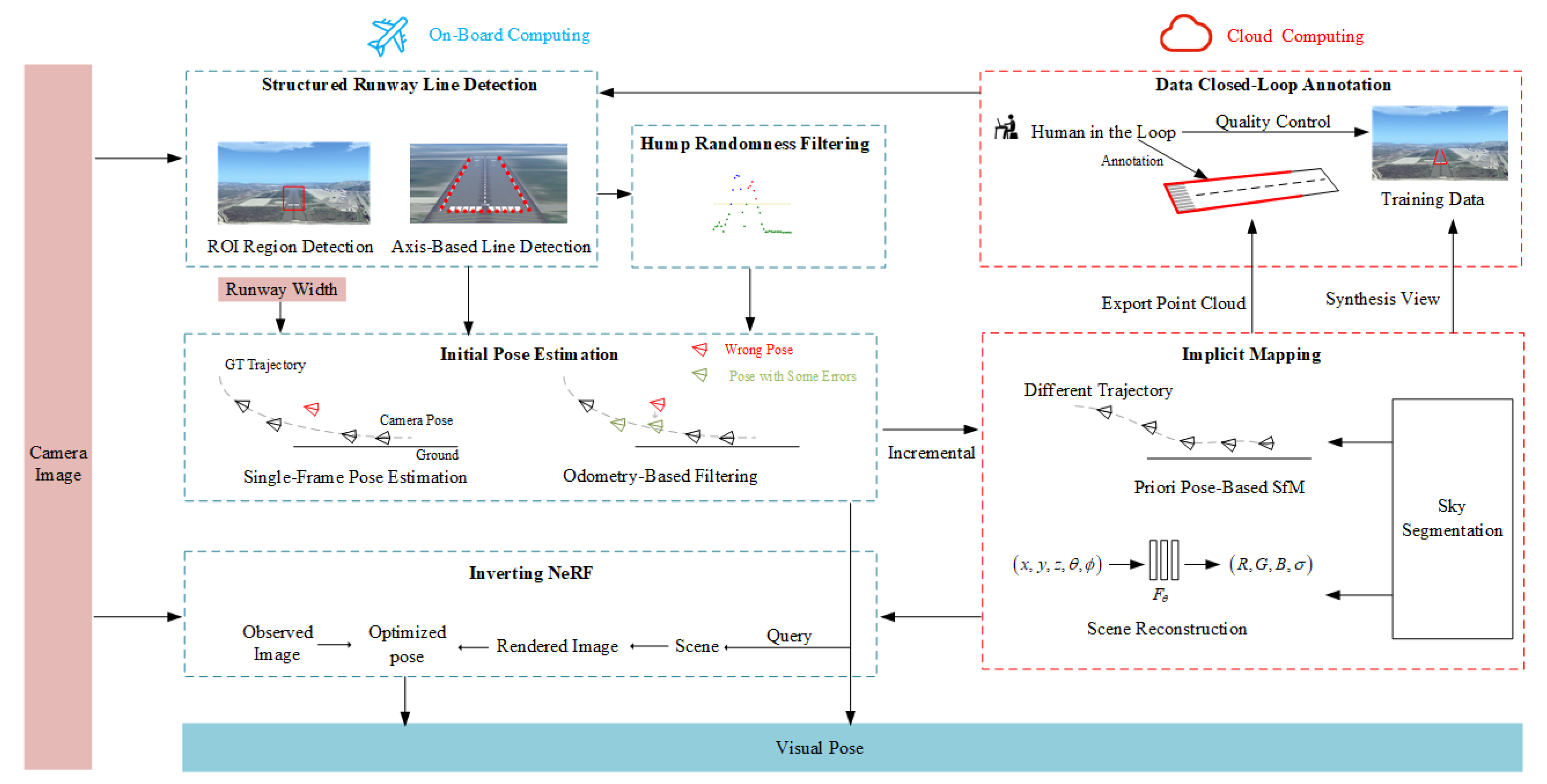
This paper proposes a solution to the pose-estimation problem in vision-only landing systems. We use the PBVS strategy to make the whole pose-estimation system robust and interpretable. To achieve higher accuracy, we propose a novel pose-estimation algorithm in a visual landing system, which is an implicit neural mapping solution (refer to Figure 1). We use camera images as input and the pose estimation as output. The runway detection, initial pose estimation, and NeRF-inverting [4] modules are computed on the on-board device (blue color in Figure 1; implicit mapping and GT annotation modules are computed on the cloud device (red color in Figure 1). The detection algorithm proposed in this paper is abbreviated as FMRLD (flexible multi-stage runway-line detection) in the experiment.

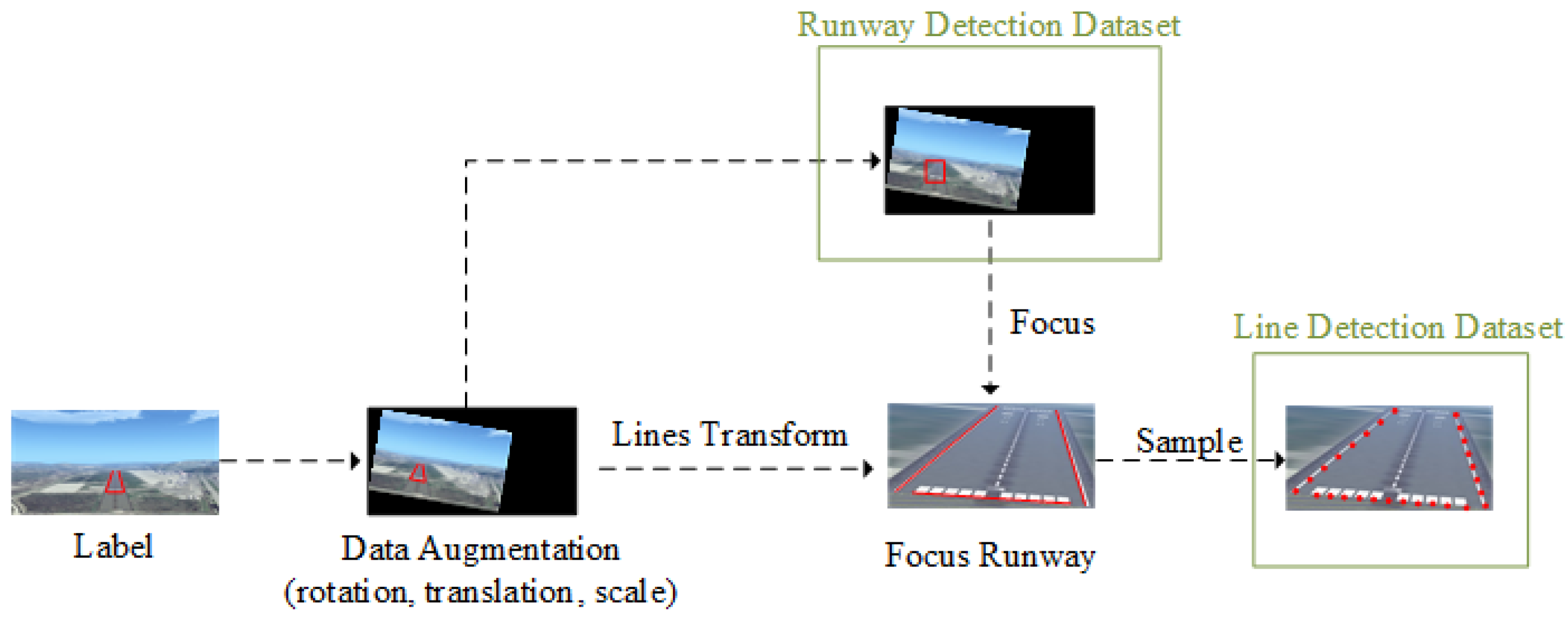
Our proposed algorithm follows the basic paradigm of pose estimation. Firstly, we perform feature extraction on the runway lines. The extracted features are then used for initial pose estimation, which is further optimized to obtain accurate estimation results. In the feature extraction phase, we use deep learning-based runway line detection methods to enhance accuracy and robustness (Section 3.1.1). 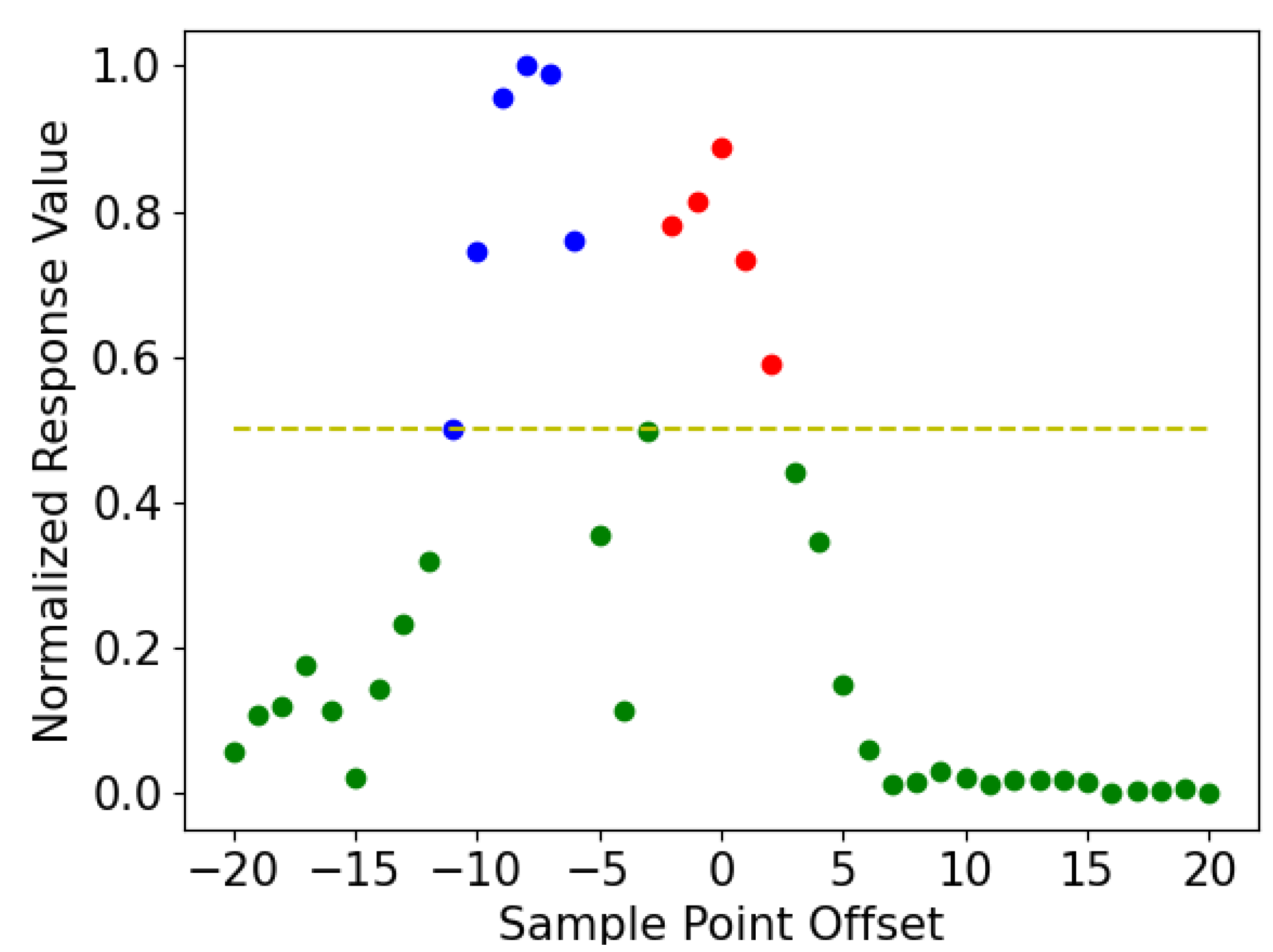These methods rely on high-quality datasets, so we utilize diverse data sources to construct datasets and perform data augmentation accordingly (Section 3.3.1). Since the accuracy of runway line detection directly affects the initial pose, we propose hump randomness filtering to refine the detection results (Section 3.1.2). During the initial pose estimation phase, we utilize the principle of multi-view geometry to estimate the pose. To ensure accuracy, we eliminate some incorrect estimation results (Section 3.2.1). The pose optimization is divided into two parts: on-board and cloud-based. On the on-board computing platform, the pose optimization results are obtained through inverting NeRF (Section 3.2.3). Meanwhile, on the cloud computing platform, the initial pose estimation results of the current trip are combined with the poses from historical trips for incremental pose optimization. The optimized results are then utilized for NeRF implicit mapping (Section 3.2.2). To address the challenges of expensive and inefficient runway data annotation, we propose a data closed-loop annotation strategy that leverages mapping results to assist in the annotation process. Specifically, we export the explicit point cloud of NeRF and allow annotators to annotate directly on the 3D point cloud. This approach significantly enhances the efficiency of data reuse compared to traditional image annotation methods. As a result, the entire algorithm operates in a closed-loop data flow (Section 3.3.2). The modules included in our proposed method are described below.

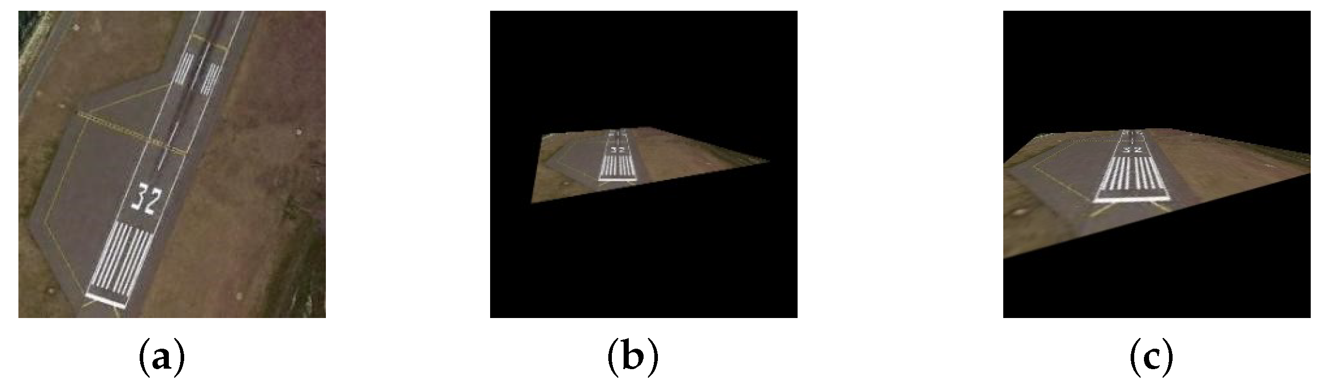
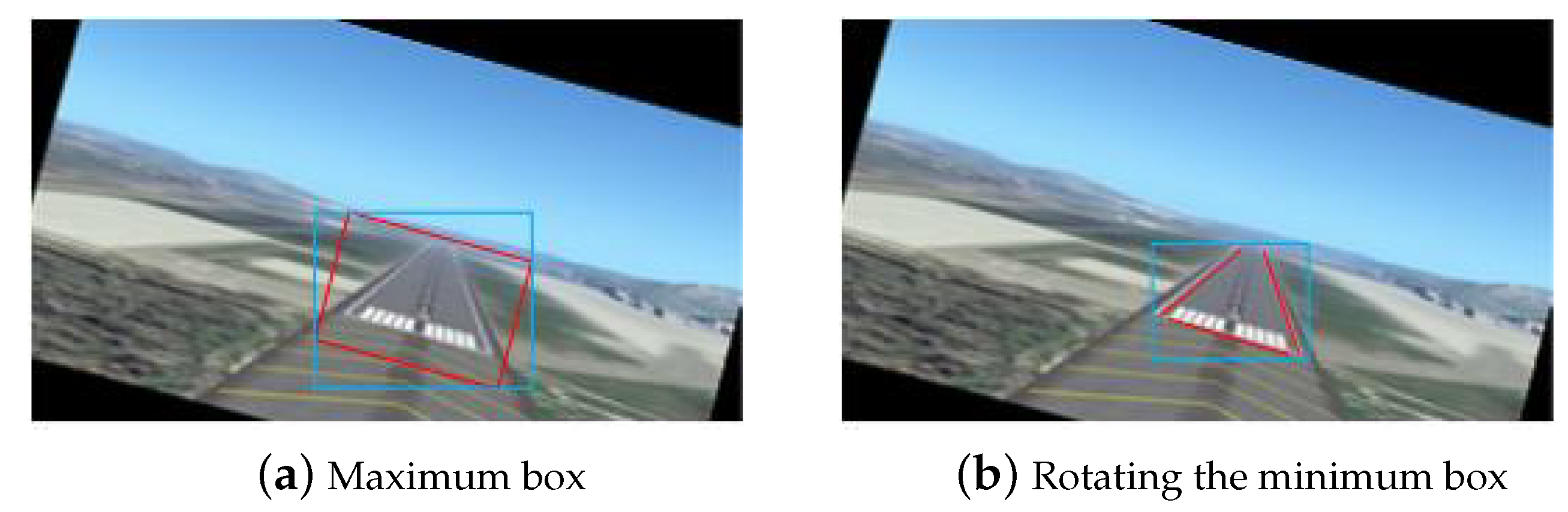
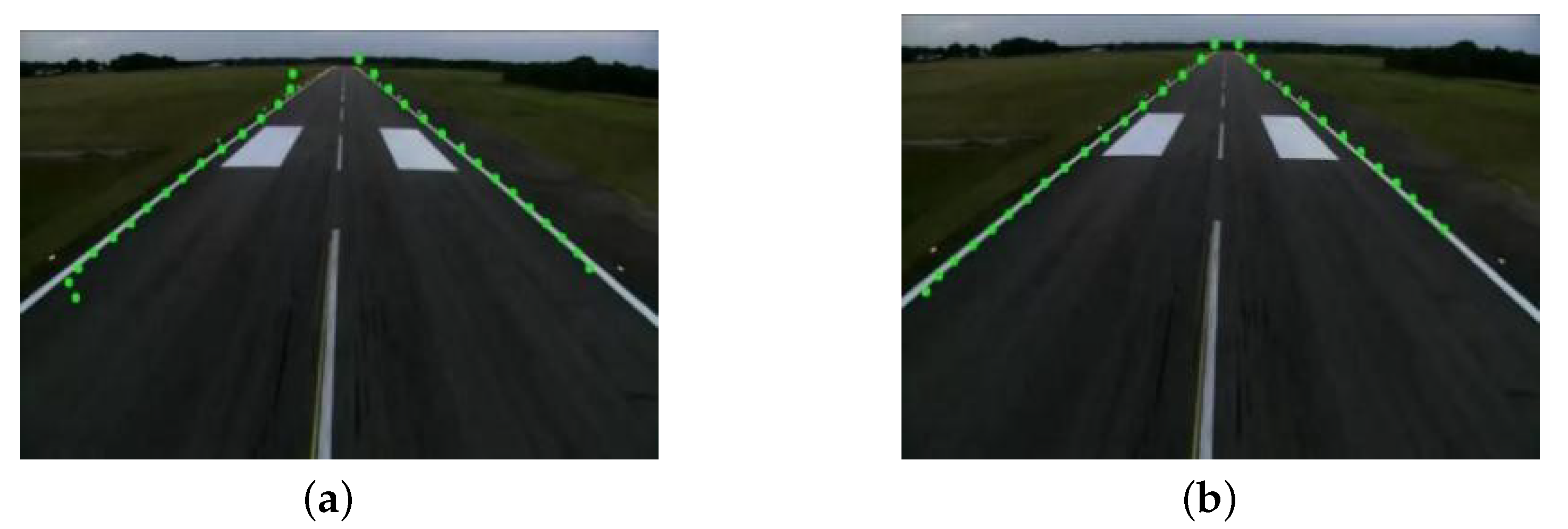
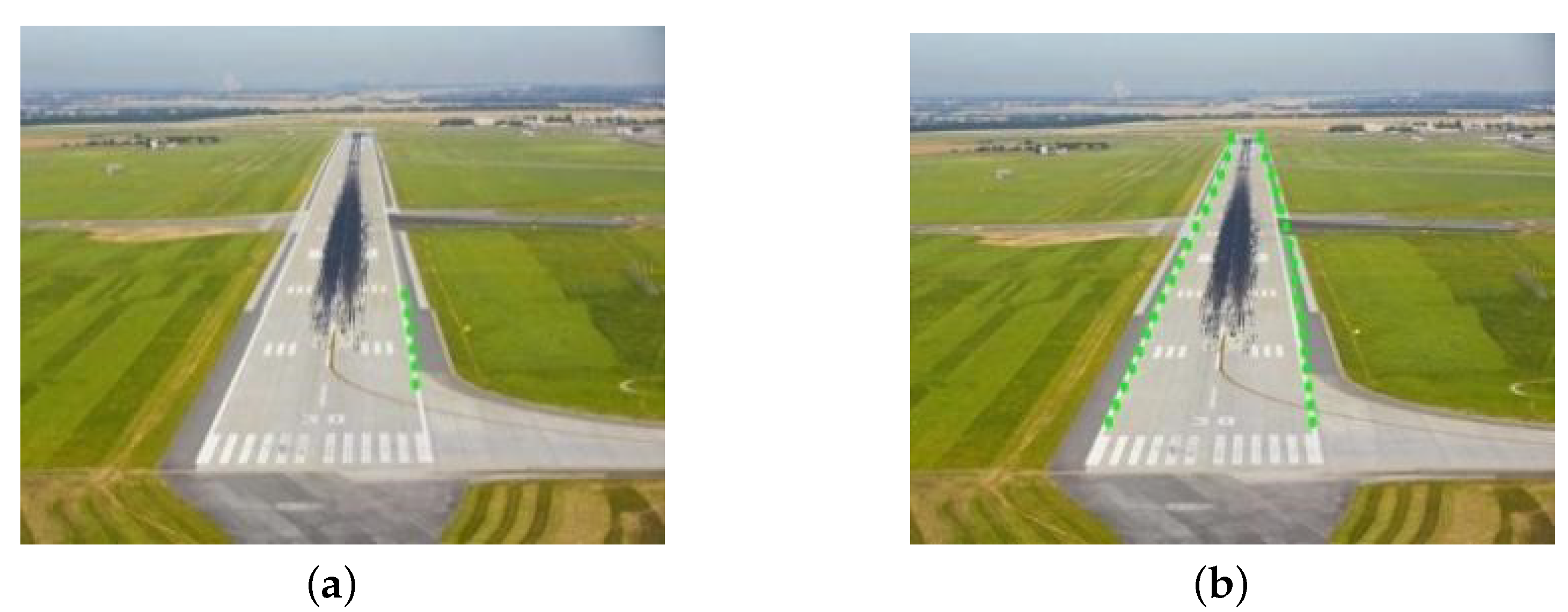
Runway detection: Accurate detection of runway lines is extremely important for navigation and positioning. Our structured runway line-detection and hump-randomness filtering modules provide consistent and reliable information on runway features. During the landing process, the visual features vary greatly among different runways, different weather conditions, and different landing phases, and these problems pose certain challenges to the accurate detection of runway lines. In this paper, our proposed coarse-to-fine accurate runway line-detection method fully considers the change in viewpoint during the landing of the aerial vehicle and the applicability of the algorithm to different scenarios. First, we use an object-detection algorithm to extract high-level semantic information about the runway, which ensures the uniform distribution of the runway in the image and facilitates the detection of subsequent runway lines. Then, we extract the left and right runway lines and the virtual start line in the focused image. We propose a column-anchor-based detection and parallel acceleration scheme for virtual start-line detection. Last, a runway line fine-tuning method based on clustering and optimization is proposed due to the randomness of detection arising from the width of the runway line. Our runway-detection module can provide good front-end detection information for pose estimation.

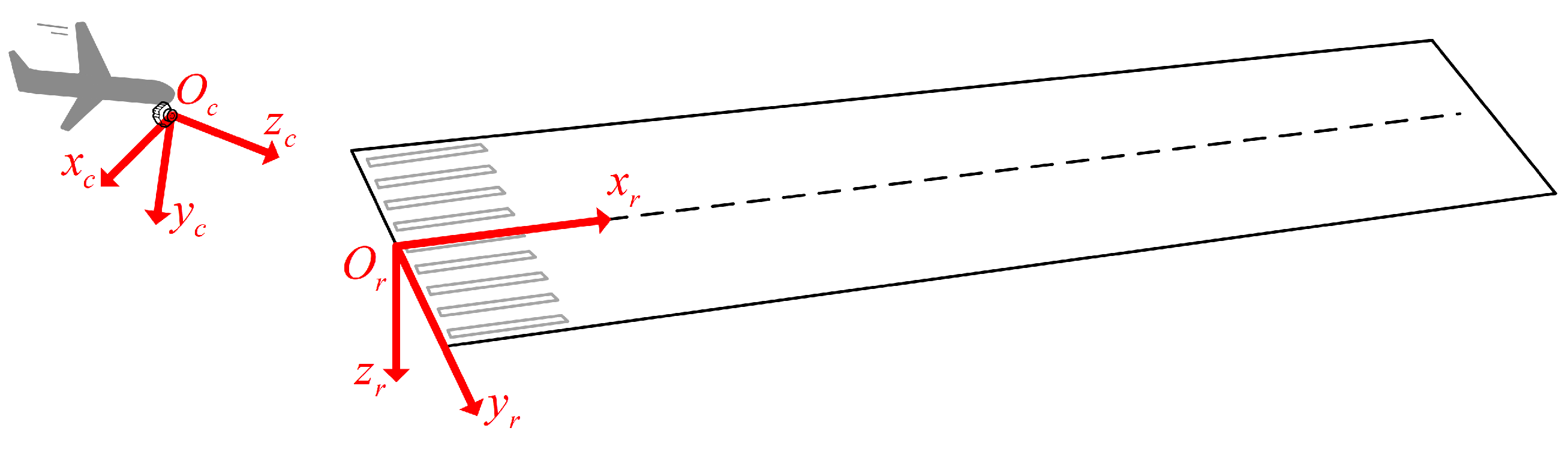
Initial pose estimation: The goal of our initial pose-estimation module is to estimate the UAV pose information with scales using a runway line feature. To obtain the scale, the module needs to input the runway width as a priori information. We use multi-view geometry, such as the vanishing point principle, to estimate the UAV’s initial pose. However, the pose is generated from a single image and does not guarantee the stability of the pose. We adopt the results of the visual odometry pose estimation as a reference to fix the instability in the initial pose estimation.

Incremental implicit mapping: The incremental implicit mapping module provides map information to the initial pose estimation and improves the accuracy of the pose estimation. It also provides high-quality point-cloud maps due to the differentiability and high fidelity of the neural radiance field (NeRF [5]). Due to the limitations of NeRF [5] in pose optimization in large scale scenes, we have split the implicit mapping module into two sub-modules: offline pose optimization and NeRF mapping. In the offline pose optimization sub-module, we have adopted the standard structure from the motion (SfM) process. However, we have two modifications. One is that we introduce a sky segmentation sub-module, which ensures that SfM does not extract feature points from the sky during the feature-extraction stage, preventing the problem of poor pose-estimation results due to feature mismatch. The other point is that we use the results of the initial pose estimation as prior information for triangulation and bundle adjustment, thus preventing the failure of pose estimation caused by local optima that SfM may fall into in large-scale scenes. In NeRF mapping, a submodule and a grid-based NeRF approach [6] are adopted. We introduce appearance embedding to ensure robustness in different weather conditions. In addition, based on some characteristics of the runway itself, we introduce regularization losses (smoothness loss, sky loss, etc.) to improve the geometry of the NeRF mapping. Please refer to Section 4 for more details.

Inverting NeRF: Inverting NeRF aims to optimize the pose-estimation result based on the implicit map when a new initial pose arrives. We use the initial pose to query the NeRF map, and we can obtain a rendered image. Meanwhile, we can also obtain the camera image on that timestamp. Using the pose as an optimization variable, we optimize the pose by constructing a loss of the observed and rendered images.

GT annotation: The runway-detection network must be trained using annotated data, which is an extremely labor-intensive process. The GT annotation module reduces the annotation cost significantly by generating a 3D point-cloud map, annotating the runway in 3D space, and then projecting it into the 2D image. At the same time, due to the differentiable representation, NeRF can synthesize images with a novel view, thus providing true 3D data augmentation. The GT annotation module achieves a closed loop of data and enhances the iterative efficiency of the whole system.

Combining the above modules, we propose a complete algorithm for estimating the pose in a vision-only landing system. The proposed algorithm has been proven effective in simulation experiments.

The main contributions of our work are follows.

(1)

A novel pose-estimation framework in a vision-only landing system is proposed, which introduces implicit mapping and ground-truth annotation modules to improve the pose-estimation accuracy and data-annotation efficiency.

(2)

We build a runway-detection pipeline. The multi-stage detection framework proposed in this paper makes full use of the features of different stages, which can guarantee semantic features and positioning ability and therefore greatly improves the runway line detection accuracy.

(3)

We present a NeRF-based mapping module in a visual landing system, whose high fidelity provides the possibility of reusing ground truth annotation, while its differentiability provides the basis for accurate pose estimation. Our NeRF-based mapping allows for the coding of different temporal styles, which is not possible with other mapping methods.

This paper is organized as follows: in Section 2, we introduce related work, including runway detection algorithms and neural radiance fields; in Section 3, we provide a detailed description of our algorithm, including implementation details of runway line detection, pose estimation, implicit mapping, and the data loop-closure module; in Section 4, we validate our proposed algorithm through experiments on runway line detection, pose estimation, and lightweight network; in Section 5, we discuss the advantages and disadvantages of our proposed algorithm, as well as future research directions; the conclusion is given in Section 6.

2. Related Work

2.1. Runway Detection

Runway detection methods can be roughly divided into three categories: detection based on a priori information, detection based on templates, and detection based on features. Feature-based detection methods have become the dominant detection method in recent years.

A Priori information-based runway detection: In a priori information-based methods, runway detection is achieved using known runway models and the aircraft attitude, and the upper limit of landing is considered in terms of safety and reliability, with the vision system primarily used as an auxiliary navigation system. The authors of [7] propose a model-based runway detection method that requires a known runway model (available through aeronautical information publication), the internal reference of the camera, and the rough pose provided by other sensors, and each line segment in the runway model can be mapped into the image using the above information. In [8], a camera model is also mapped to the image first, but unlike [7], the ROI given in this paper is the ROI of the smallest rectangle containing the left and right runway lines rather than the ROI of each segment of the runway model line. However, in tasks such as emergency landings, the initial attitude estimation is noisy and the sensor type is limited, and the model-based runway detection is less effective in this case.

Template-based runway detection: Template-based runway line detection uses the comparison of the query image and the template image to achieve detection. In [9], LSD is used for line feature extraction, and chamfer matching is later used to achieve runway search, but due to the limitations of template matching itself, the template often cannot adapt to the large changes in view during the landing process. The authors of [10] used a manually designed template to find the ROI and rotates the image in different directions after obtaining the binarized edge gradient map. Then, the sum of the pixel values in different columns is counted to find their peaks, and the peaks are clustered under different rotation angles. Finally, the clustering centers are mapped to straight lines in the original image to achieve runway line detection. Template-based detection methods are poorly generalized and often fail because they are more sensitive to runway geometry and light conditions.

Feature-based runway detection: Runway line detection based on image features is mainly achieved using visual images. Unlike remotely sensed runway detection [11], the proportion of the runway in the image changes continuously in the landing scenario, and the left and right runway edges no longer have parallel characteristics. In [12], the HSV color model and LSD algorithm were used to detect non-standard airfields, and the paper concluded that using the HSV color model could achieve better detection results than the RGB color model. In [13], ROIs are formed by corner-point detection and clustering, and then a neural network is used to classify these ROIs to determine the location of runway edges. However, it is a challenge to choose the number of clusters effectively. The authors of [14] use an end-to-end segmentation network for runway line detection and a self-attention module to enhance the segmentation, while a lightweight network is used to ensure real-time detection, but the paper does not give the impact of detection on subsequent tasks.

None of the above detection methods consider the effectiveness of detection under large viewpoint changes during landing, resulting in these methods only being effective when there is a small variation in perspective and therefore requiring different detection models to be set up for different landing stages (e.g., detection parameters need to be fine-tuned). Additionally, the detection of the starting line can enhance pose estimation performance; however, the above-mentioned methods often fail to detect the virtual start line as it often does not exist. Our proposed method overcomes these problems effectively and provides accurate and reliable runway line detection results.

2.2. Neural Radiance Field

NeRF is a recent breakthrough in the field of computer vision that allows for the generation of highly realistic 3D models of objects and scenes from 2D images. The method works by training a deep neural network to predict the radiance at any point in 3D space, given a set of images and corresponding camera poses. This allows for the creation of photorealistic renderings of objects and scenes from any viewpoint and even enables the synthesis of novel views that were not captured by the original images.

NeRF has been applied to a wide range of applications, including virtual reality, augmented reality, and robotics. It has also been used to generate 3D models of real-world objects and scenes, such as buildings, landscapes, and even human faces.

While NeRF has shown remarkable success in generating high-quality 3D models from a small number of images, it faces several challenges when applied to large-scale scenes.

Computation complexity: The continuity expression of NeRF and the weak assumption of spatial consistency result in slow convergence during training and while requiring large networks to compute the RGB and density of spatial sampling points, which also leads to the slow inference speed of the network. In large-scale scenes, a large number of points in the scene need to be calculated, so the computational requirements can become prohibitively large.

To address the challenge, several approaches have been proposed. It has been shown in recent research that grid-based representations can be used to speed up the training and inference of NeRF significantly. Plenoxels [15] store density values and colors directly on a voxel grid, rather than relying on an MLP network. Instant-NGP [6] greatly improves the training efficiency by utilizing hash encoding and multi-resolution mechanisms. F2NeRF [16] delves deep into the mechanism of space warping to handle unbounded scenes and achieves fast free-viewpoint rendering by allocating limited resources to highlight the necessary details.

Few shot: The original NeRF method requires a 360-degree view of the target object, allowing the network to effectively learn the geometric properties of the scene due to the large amount of co-visible areas. However, in some scenes, the number of input views is limited or the view directions are relatively uniform, which may deceive the network and prevent it from learning the correct geometric information from the images. RegNeRF [17] alleviates artifacts caused by the sparse input by adding regularizations on both geometry and appearance. DS-NeRF [18] and Urban-NeRF [19] improve the geometry of the scene by adding depth supervision.

During the visual landing process, the observation viewpoint is relatively uniform and falls into this category. To address these challenges, prior regularization constraints or depth supervision are often required to be added to the network.

Different resolutions: When there are multiple resolutions present in the input images, NeRF can exhibit blurring and aliasing. MipNeRF [20] solves this problem effectively by using cone sampling. In the process of visual landing, there is a significant difference in resolution between the early and late stages of landing. Therefore, our paper adopts a MipNeRF-based approach to address this issue.

3. Method

3.1. Multi-Stage Flexible Runway Detection

Our multi-stage runway-line-detection algorithm constructed in this paper follows the design principle from coarse to fine, which can largely improve the reliability and accuracy of runway-line detection. The first stage uses the object-detection algorithm, which can effectively extract the high-level semantic information of the runway. By extracting ROIs (regions of interest), it can ensure the uniform distribution of the runway in the image and facilitate the detection of subsequent runway lines. The second stage of the runway-line-detection algorithm is used to extract left and right runway lines and the virtual start line in the focused image, and the extracted runway lines are described in the form of point sets. The runway-line-detection algorithm does not use object segmentation techniques but rather row- and column-specific classification, which is able to reduce the computational effort and increase the inference performance. The third stage mainly adjusts the results of runway-line detection using pixel tuning and sub-pixel tuning to ensure that the detection results of runway lines are attached to the inner edges of the runway lines, thus effectively reducing the randomness of runway line detection.

3.1.1. Structured Runway-Line Detection

We adopt a row anchor-based [21] mechanism for runway-line detection, which samples the image in equally spaced rows, then uses the sampled rows as anchor rows and classifies several adjacent columns into the same grid. With these two processing techniques, the computational effort of the algorithm can be significantly reduced. Below, the network feature of the image is denoted as F, the runway-line-detection classifier is denoted as f, and the predicted results of the runway line are denoted as P.

For the i-th runway line and the $j_1$-th row anchor, the prediction result can be expressed as:

$$P_i^{j_1}=f_i^{j_1}\left(F\right),$$

(1)

where the number of row anchors is $a_r$ the number of column grids is $n_c$, and $P_i^{j_1}$ is an $n_c+1$ dimensional vector, where the extra dimension is used to indicate the presence or absence of the runway line.

However, the method does not allow for virtual start-line detection, as the slope of the start line is close to zero and the start line can not be effectively detected using the row anchor. In order to solve this problem, we design a column-anchor-based virtual start-line-detection method.

Similar to row anchors, column-anchor detection is defined as follows. For the i-th runway line and the $j_2$-th column anchor, the prediction can be expressed as:

$$P_i^{j_2}=f_i^{j_2}\left(F\right),$$

(2)

where the number of column anchors is $a_c$, the number of row grids is $n_r$, and $P_i^{j_2}$ is an $n_r+1$ dimensional column vector.

Although such a design works in theory, the left and right runway lines and the virtual start line need to be predicted separately; i.e., two sets of models are required, which is detrimental to the reuse of network features, the management of the network model, and parallel GPU acceleration. Considering the pairwise characteristics between column and row, we propose an ingenious design approach to unify the left and right runway line and the start line in a unified detection framework.

The left runway line, right runway line, and the virtual start runway line are numbered i as 1–3, respectively, and then the prediction can be expressed in the following form:

$$\left\{\begin{array}{c}{P}_1^{j_1}=f_1^{j_1}\left(F\right)\\ P_2^{j_1}=f_2^{j_1}\left(F\right)\\ P_3^{j_2}=f_3^{j_2}\left(F\right)\end{array}\right.$$

(3)

To ensure matching dimensions, two merging methods can be generated, which are:

$$\left\{\begin{array}{c}{a}_r=n_r\\ a_c=n_c\end{array}\right.$$

(4)

or:

$$\left\{\begin{array}{c}{a}_r=a_c\\ n_c=n_r\end{array}\right.$$

(5)

If the form of Equation (4) is used, the $P_1^{j_1}$, $P_2^{j_1}$, and $P_3^{j_2}$ column vectors may have different dimensions, and in this case, if the different runway lines are processed uniformly, there will be invalid elements in the matrix P. If the form of Equation (5) is used, the $P_1^{j_1}$, $P_2^{j_1}$ and $P_3^{j_2}$ column vectors have the same dimension, in which case all the data in the matrix P are valid, and P can be expressed as:

$$P=\left[\begin{array}{ccc}{P}_1^{j_1}& P_2^{j_1}& P_3^{j_2}\end{array}\right]=\left[\begin{array}{ccc}{f}_1^{j_1}\left(F_2\right)& f_2^{j_1}\left(F_2\right)& f_3^{j_2}\left(F_2\right)\end{array}\right]$$

(6)

We use this combined form to unify the three runway lines and then interpret them differently in the post-processing stage.

Although the detection of three runway lines can be achieved using the above approach, in order to enable the runway-line-detection network to learn more essential features and achieve better generalizability, we add regular terms based on the geometric properties of the runway. There is a certain constraint relationship between the left and right runway lines. Due to perspective, the closer one gets to the top of the image, the closer the left and right runway lines are from the perspective of the image. For the i-th runway line and the $j_1$-th row anchor, the probability can be expressed as:

$$p_i^{j_1}=softmax\left(P_i^{j_1}\right)$$

(7)

So the location prediction results are:

$$L_i^{j_1}=\sum _{k=1}^{n_c}k·p_i^{j_1}\left(k\right)$$

(8)

For the same anchor row, the difference between the predicted positions of the left and right runway lines is:

$$D^{j_1}=L_1^{j_1}-L_0^{j_1},\mathrm{s}.\mathrm{t}.j\in \left[0,h\right]$$

(9)

The difference in distance between the left and right runway lines between adjacent anchor rows is expressed as:

$$\Delta D^{j_1}=D^{j_1+1}-D^{j_1},\mathrm{s}.\mathrm{t}.j_1\in \left[0,h-1\right]$$

(10)

Ideally, no loss is caused in the case of $\Delta D^{j_1}>0$, while a loss is caused when $\Delta D^{j_1}<0$. However, in the actual detection process, a certain tolerance threshold needs to be set. The reason for designing the threshold is mainly due to the fact that the constraint of a zero threshold is too strict, and the use of a zero threshold may reduce the performance of the detection. Assuming that the tolerance threshold is T, then, for each anchor row, the loss can be expressed as:

$$M^{j_1}=0.5\times \left(\left|\Delta D^{j_1}+T\right|-\Delta D^{j_1}-T\right),\mathrm{s}.\mathrm{t}.j_1\in \left[0,h-1\right]$$

(11)

Therefore, the correlation loss of the left and right runway lines can be expressed as:

$$Los{s}_{relation}=\sum _{j_1=1}^{h-1}{∥M^{j_1}∥}_1$$

(12)

For the starting runway line, which is itself a virtual line, the distortion is prevented by adding a linear constraint-regularization term. The experimental results show that the structured loss of the left and right runway lines proposed in this paper and the linear loss of the starting line can improve the generalization.

3.1.2. Hump Randomness Filtering

The accuracy of the runway-line detection directly affects the subsequent position estimation. However, as the result of the width of the runway lines themselves, there is randomness in the location of the detection points in the structured runway-line detection. During the initial period of access to the visual landing system, the runway lines occupy fewer pixels in the image, but the positioning is more sensitive to small fluctuations in detection, and when the UAV is about to reach the ground, the runway lines occupy a certain width in the image, and if each runway is still considered as one edge in this case, it will produce great detection uncertainty. In this paper, the left and right runway line edges are absorbed toward the inner side of the runway, which effectively solves the problem of detection uncertainty.

Although there are off-the-shelf edge-detection algorithms, such as Sobel [22], Canny [23], etc., such generic edge-detection algorithms do not have direction selection characteristics and tend to introduce non-runway edge information, which causes some interference in the subsequent steps. In addition, since the general location of the runway line is already given in the second stage, there is no need to take the gradient of the whole map, but only to find the gradient at some specific locations, which can reduce the computational effort.

In order to enhance the gradient information of runway edges while suppressing the gradient information of non-runway edges, a directional gradient strategy is proposed in this section. The initial slope of the runway line $k_{rough}$ can be determined from the detection points of the previous stage, so the directional gradient convolution kernel is determined based on the initial slope. Specifically, consider convolution kernel $K_e$ as an $N\times N$ grid, given a straight line passing the center of the convolution kernel with slope $k_{rough}$. The straight line divides the original grid into three categories: grids on the top side of the straight line, grids on the bottom side of the straight line, and grids passing through the straight line. The values for these three types of grids are set to 1, −1, and 0, respectively. After the convolution kernel K is solved for, a directional gradient image can be obtained.

The detection point $\left(x_0,y_0\right)$ is sampled in the directional gradient image along the orthogonal direction $y=n\left(x\right)$ to the left and right for $N_0$ pixels. The sampling sequence is defined as:

$$S_{(x_0,y_0)}=\left[s_0...s_{2\times N_0}\right],$$

(13)

where $s_t\left(t=0,...,2\times N_0\right)$ denotes the gradient value on the specific sample point. $S_{(x_0,y_0)}$ is normalized to obtain $S{n}_{(x_0,y_0)}$.

The values of $S{n}_{(x_0,y_0)}$ are first filtered to remove the points whose amplitude is less than the specified threshold, e.g., 0.5, and then the remaining points are clustered by two-dimensional K-means++ [24]. The clustering results are shown in Figure 2. Assuming that the peaks of two categories are $r_i^{max}$, where $i=0,1$, and then we can obtain the adjust points, and the result is used as initial value for subsequent optimization, which can be expressed as:

$$\left\{\begin{array}{c}{x}_i^{rough}=x_0+\underset{\Delta x}{\arg \max }{r}_i^{max}\\ y_i^{rough}=n\left(x_i^{rough}\right)\end{array}\right.$$

(14)

Ideally, the edge gradient of an image is an impulse signal, but due to factors such as image blurring and filtering, the edges often do not conform to this model. We assume that the change in the image edge gradient conforms to the Gaussian model. Under this assumption, the horizontal coordinate corresponding to the peak of the Gaussian distribution is the edge position. For the runway line, there is a certain width itself, and the points on the runway line may be affected by both the left edge and the right edge. A hump model is proposed to deal with the sub-pixel fitting of the runway to obtain more accurate detection results. $B\left(\Delta x\right)$ is defined as:    

$$B\left(\Delta x\right)=\frac{k_0}{\sqrt{2\pi {\sigma }^2}}\left(exp\left(-\frac{{(\Delta x-{\mu }_0)}^2}{2{\sigma }^2}\right)+exp\left(-\frac{{(\Delta x-{\mu }_1)}^2}{2{\sigma }^2}\right)\right),$$

(15)

where the horizontal coordinates of the two peaks, denoted ${\mu }_0$ and ${\mu }_1$, respectively, are the coordinates of the left and right edges of the runway to be sought. The standard deviation of the Gaussian function is denoted as $\sigma$, which is shared by two Gaussian functions.

We use the Levenberg–Marquardt method to optimize. In order to speed up the optimization and prevent the algorithm from falling into local optima, we add a regular term. Specifically, the distance of the peak points actually reflects the width of the runway line, which is actually relatively narrow. By constraining the distance between the two peaks, the result can be made to satisfy the actual physical scene. The experiments show that the regular term can effectively prevent the algorithm from falling into a local optimum, and the optimization problem can be described as follows:

$$\psi \ast =\underset{\psi }{\arg \min }\frac{1}{2N_0+1}\sum _{i=-N_0}^{N_0}{\left(B_{\psi }\left(i\right)-S{n}_{\left(x_0,y_0\right)}\left[i+N_0\right]\right)}^2+\lambda {∥{\mu }_0-{\mu }_1∥}_2,$$

(16)

where the parameters are defined as $\psi =\{{\mu }_0,{\mu }_1,\sigma ,k_0\}$, the model under a particular set of parameters p is defined as $B_{\psi }(\Delta x)$, and $\lambda$ is the regularization coefficient. The initial values of ${\mu }_i^{initial}$ are selected as $\underset{\Delta x}{\arg \max }{r}_i^{max}$, where $i=0,1$.

After obtaining ${\mu }_i$, similarly to Equation (14), we can obtain $(x_i^{fine},y_i^{fine})$. We then use the following criteria to check the optimized result, which is:

$$\left|{\mu }_i-\underset{\Delta x}{\arg \max }{r}_i^{max}\right|<\tau$$

(17)

We set $\tau$ to 1 or less because the optimized model is fine-tuned sub-pixel and an adjustment value greater than 1 is considered unreasonable. When the optimization result does not satisfy this criterion, the initial value is used as the final result.

The hump randomness filtering algorithm is shown in Algorithm 1.

Algorithm 1 Hump Randomness Filter

Input:  Detection Points Set $\mathbf{S}$, Image $\mathbf{I}$; Output:  Adjust Points Set ${\mathbf{S}}^{\prime }$   Directional convolution kernel $K_e\leftarrow$ Detection points set $\mathbf{S}$;   for s in S do       Sequence $Q\leftarrow$ Sampling along the gradient direction for point s       Sequence $S_n\leftarrow$ Get the directional gradient value of each point in Q using kernel $K_e$       Initialize ${\mu }_i^{initial}\leftarrow$ Clustering with $S_n$ to get two peak       ${\mu }_i\leftarrow$ Using Sequence $S_n$ and ${\mu }_i^{initial}$ to optimize the hump model       if $\left|{\mu }_i-{\mu }_i^{initial}\right|<\tau$ then           Use optimized parameters to get $S^{\prime }$       else           Use init parameters to get $S^{\prime }$       end if   end for

3.2. Implicit Reconstruction-Based Pose Estimation

3.2.1. Initial Pose Estimation

We use runway line features to initialize the UAV pose. The runway coordinate system and camera coordinate system are defined as shown in Figure 3. The origin $O_r$ of the runway coordinate system is chosen as the midpoint of the runway start line, the $x_r$ points from $O_r$ to the front of the runway, and $z_r$ starts from $O_r$ and is perpendicular to the runway plane, and $y_r$ can be determined according to the right-handed coordinate system.

The origin $O_c$ of the camera coordinates system is located at the optical center of the camera, the $z_c$ points from $O_c$ to the camera directly in front, $x_c$ points to the camera directly to the right, and $y_c$ can be determined according to the right-handed coordinate system.

The positions of the 3D points in the runway coordinate system and the positions of the points in the pixel coordinate system are mathematically related as follows:

$${\overrightarrow{v}}_p=\frac{1}{Z_c}K{R}_{cr}\left[I_{3\times 3} |-{\overrightarrow{t}}_{cr}\right]\left[\begin{array}{c}{\overrightarrow{v}}_r\\ 1\end{array}\right]=\frac{1}{Z_c}P\left[\begin{array}{c}{\overrightarrow{v}}_r\\ 1\end{array}\right],$$

(18)

where $P=K{R}_{cr}\left[I_{3\times 3}\right|-{\overrightarrow{t}}_{cr}]$ is the projection matrix, $R_{cr}$ denotes the rotation matrix from the runway coordinate system to the camera coordinate system, K is the camera’s intrinsic matrix, and ${\overrightarrow{t}}_{cr}$ denotes the coordinates of the origin of the camera coordinate systems in the runway coordinate system. Assuming that the slope and bias of the runway line in the pixel coordinate system are denoted as $k_i$ and $b_i$, where i is selected from $\{l,r,h\}$, which denote the left runway line, the right runway line, and the start runway line, respectively. The following location algorithm is given without proof [25,26]:

$${\overrightarrow{A}}_i=\left[\begin{array}{ccc}{k}_i& -1& b_i\end{array}\right]K{R}_{cr}$$

(19)

The first three columns of ${\overrightarrow{A}}_i$ are denoted as $a_i^1$, $a_i^2$, $a_i^3$, respectively, and the width of the runway is W. The positioning result can be expressed as follows:

$$\left\{\begin{array}{c}\left[\begin{array}{c}{y}_{cr}\\ z_{cr}\end{array}\right]={\left[\begin{array}{cc}1& a_l^3/a_l^2\\ 1& a_r^3/a_r^2\end{array}\right]}^{-1}\left[\begin{array}{c}-W/2\\ W/2\end{array}\right]\hfill \\ x_{cr}=-a_l^3{z}_{cr}/a_l^2\hfill \end{array}\right.$$

(20)

With this method, the real width of the runway and the relative poses between the runway and the camera need to be given. The attitude of the camera can be obtained using an IMU and magnetometer, but the attitude of the runway is often difficult to obtain directly, so the relative attitude of the runway and the camera is more difficult to obtain. Below is a method to estimate the relative attitude of the UAV and the runway based on the runway line features [27].

The extinction points of the left and right runway lines are:

$$v_{lr}^p=\left(\begin{array}{cc}(b_r-b_l)/(k_l-k_r)& (k_l{b}_r-k_r{b}_l)/\left(k_l-k_r\right)\end{array}\right)$$

(21)

And the extinction point $v_s^p$ of the starting line can be obtained from Equation (22):

$$\left[\begin{array}{c}{\left(v_{lr}^p\right)}^T\left(K^{-\mathrm{T}}{K}^{-1}\right)\\ l_s^T\end{array}\right]v_s^p=0$$

(22)

Based on the above, the rotation matrix $R_{cr}$ can be expressed as follows:

$$R_{cr}=\left[\begin{array}{ccc}\frac{1}{{\alpha }_1}{K}^{-1}{v}_{lr}^p& \frac{1}{{\alpha }_2}{K}^{-1}{v}_s^p& \frac{1}{{\alpha }_3}\left(K^{-1}{v}_{lr}^p\right)\times \left(K^{-1}{v}_s^p\right)\end{array}\right]$$

(23)

In Equation (23), ${\alpha }_1$, ${\alpha }_2$, and ${\alpha }_3$ are normalized coefficients.

Based on the above, we obtain the single-frame pose of the UAV camera in the runway coordinate system. For the k-th frame, the pose estimated using above method can be abbreviated as ${\Gamma }_k^{\mathrm{frame}}$.

However, a single-frame pose can suffer from unstable pose estimation. We used a visual odometer-based filtering method to remove the jumps. We initialized the scale of the monocular odometer using a single-frame pose. In feature extraction, we use the trained sky segmentation model to remove invalid feature points in the sky and increase the proportion of feature points in the runway area. Using the odometer’s pose-estimation results, we are able to obtain pose transformation from k to $k+1$, denoted as ${\Gamma }_{k\to k+1}^{odom}$. Meanwhile, we are able to obtain ${\Gamma }_{k\to k+1}^{\mathrm{frame}}={\Gamma }_{k+1}^{\mathrm{frame}}{\left({\Gamma }_k^{\mathrm{frame}}\right)}^{-1}$. Then, we use the similarity metric ${\Gamma }_{k\to k+1}^{odom}{\left({\Gamma }_{k\to k+1}^{\mathrm{frame}}\right)}^{-1}$ to determine whether to use a single-frame pose. If the threshold condition is not met, the odometer pose is used as the estimation pose. We denote the result as ${\Gamma }_k^{\mathrm{initial}}$.

3.2.2. Implicit Mapping

Cloud computing, like offline computing, can see all the pose data of the previous flight trajectories in one batch, while cloud-based platforms have more computing resources, which is an advantage of cloud-based mapping and pose estimation over the onboard platform. We propose a scheme to reconstruct the implicit map using an implicit radiance field and optimize the UAV’s pose attitude online.

We use ${\Gamma }^{\mathrm{initial}}$ as an a priori pose and use SfM for pose optimization [28]. During feature extraction, we use the segmentation model to remove sky feature points and moving objects such as birds. The feature matching is made more efficient by using a priori poses to guide this process. In the triangulation process, the SfM process itself has a real scale due to the a priori poses. During bundle adjustment, a priori poses are used as optimization regularization to prevent failure. In landing scenarios, there are often multiple trips with different flight paths, and it is important to merge them. One strategy is to optimize all trajectory poses together. However, this is computationally inefficient and often leads to optimization failure due to the high degree of freedom in the optimization process. We adopt a progressive merging strategy, where new trip data arrive and are first reconstructed separately and then merged with existing results. The experimental results show that the feature point extraction strategy, a priori poses, and incremental reconstruction can effectively improve the reconstruction accuracy of the SfM. We denote the pose optimization result as ${\Gamma }^{\mathrm{opt}}$. This result is used for NeRF reconstruction.

Assume that the RGB color of a certain pixel is ${\mathbf{C}}_{\mathbf{t}}$; to render this pixel in NeRF, a ray $\mathbf{r}\left(t\right)=\mathbf{o}+t\mathbf{d}$ is emitted from the camera’s center of projection $\mathbf{o}$ in the direction $\mathbf{d}$ that passes through the pixel, and distance $t\in (t_n,t_f)$, where $t_n$ and $t_f$ are the predefined near and far distances. A sampling strategy is used to obtain the sampled $t_k$. For each distance $t_k\in t$, the 3D position can be expressed as $\mathbf{x}=\mathbf{r}\left(t_k\right)$. Then, a positional encoding strategy is used to improve rendering quality. The output of the specific sampling points k after passing through the neural radiance field are RGB colors ${\mathbf{c}}_{\mathbf{k}}$ and a density ${\sigma }_k$, which can be expressed as:

$$\left[{\sigma }_k,{\mathbf{c}}_k\right]=\mathrm{MLP}\left(\gamma \left(\mathbf{r}\left(t_k\right)\right)\right),\forall t_k\in t,$$

(24)

where MLP represents the neural radiance network, while $\gamma (·)$ denotes the positional encoding function.

The estimated densities and colors are utilized for approximating the volume-rendering integral through numerical quadrature, which is discussed in the volume-rendering review by Max [29]:

$${\mathbf{C}}_p\left(\mathbf{r}\right)=\sum _k{T}_k\left(1-exp\left(-{\sigma }_k\left(t_{k+1}-t_k\right)\right)\right){\mathbf{c}}_k,$$

(25)

in which $T_k=exp\left(-{\displaystyle \sum _{k^{\prime }<k}}{\sigma }_{k^{\prime }}\left(t_{k^{\prime }+1}-t_{k^{\prime }}\right)\right)$, and ${\mathbf{C}}_p\left(\mathbf{r}\right)$ is the final predicted color of the pixel. During the training of the NeRF network, the predicted pixel value ${\mathbf{C}}_p\left(\mathbf{r}\right)$ is minimized with respect to the true pixel value ${\mathbf{C}}_t\left(\mathbf{r}\right)$ using gradient descent.

Theoretically, we have the optimized poses ${\Gamma }^{\mathrm{opt}}$, camera intrinsic matrix $\mathbf{K}$, and the corresponding images to perform the NeRF implicit reconstruction. However, there are some challenges in our specific scenario. Problem I is that the drastic changes in the viewpoint during landing and the large variation in runway resolution are also difficult problems for the NeRF model. Problem II is the problem of large-scale scenes: visual landing requires the representation of large scenes, which the original NeRF model is unable to handle. Problem III is the issue of appearance style: landing scene data may come from different times, and if this problem is not effectively addressed, it can affect the performance of the implicit map. Problem IV: due to the few viewpoints during landing, it is difficult to learn the geometric information of the scene in the mapping process.

To address Problem I, we adopt the approach proposed in MipNeRF [20], using conical frustum instead of rays in NeRF to alleviate the aliasing issues caused by multi-resolution.

To address Problem II, we utilize the scene parameterization mechanism from MipNeRF360 [30]. Specifically, we achieve coordinate transformation through defining $\mathrm{contract}(·)$:

$$\mathrm{contract}\left(\mathrm{x}\right)=\left\{\begin{array}{cc}\mathrm{x}& ∥\mathrm{x}∥⩽1\\ (2-1/∥\mathrm{x}∥)(\mathrm{x}/∥\mathrm{x}∥)& ∥\mathrm{x}∥>1\end{array}\right.$$

(26)

This approach allows us to compress the range of spatial points from $\left[0,+\infty \right)$ to $\left[0,2\right)$. By choosing an appropriate unit scale, we can effectively represent unbounded scenes.

To address Problem III, we apply the appearance-embedding mechanism from NeRF-W [31] to our approach. NeRF-W assigns a unique appearance encoding to each image and obtains a corresponding word vector. This vector is then fed into a multilayer perceptron for backpropagation optimization, resulting in an appearance encoding that captures the style of the current image. However, unlike the “wild” images in NeRF-W, the images in the visual landing system maintain a consistent style throughout each trip. By setting the same appearance encoding for all images in a trip, we reduce the degree of freedom in appearance encoding and allow it to capture the essential features of the appearance. We denote the appearance encoding as ${\mathbf{e}}_i$, where i denotes the i-th trip. After the appearance embedding is incorporated, Equation (24) can be rewritten as:

$$\left[{\sigma }_k,{\mathbf{c}}_k\right]=\mathrm{MLP}\left(\gamma \left(\mathbf{r}\left(t_k\right)\right),{\mathbf{e}}_i\right),\forall t_k\in t$$

(27)

To address the problem IV, we add some regularization constraints based on the physical properties of the real scene to limit the geometric degrees of freedom.

The sky’s depth is considered to be infinite. Since the sky often lacks effective features, if the depth of the sky is not constrained, many floaters will appear in the scene. By adding regularization constraints to the sky, this problem can be alleviated [19]. All the rays belonging to the sky can be obtained based on the sky segmentation model, denoted as the set $R_s$, which contains $n_s$ elements, and we define sky loss $L_{sky}$ to encourage sky rays to have zero density:

$$L_{sky}=\frac{1}{n_s}\sum _{\mathbf{r}\in R_s}\sum _k{\left[T_k\left(1-exp\left(-{\sigma }_k\left(t_{k+1}-t_k\right)\right)\right)\right]}^2$$

(28)

The runway area, which is the focus of our attention, conforms to the assumption of planar smoothness. Therefore, we use the geometry regularization [17] to constrain the geometry of the runway. The depth of NeRF is generally represented as:

$$d_p\left(\mathbf{r}\right)=\sum _k{T}_k\left(1-exp\left(-{\sigma }_k\left(t_{k+1}-t_k\right)\right)\right)t_k$$

(29)

All the rays belonging to the runway can be obtained based on the runway-detection model, denoted as the set $R_r$, which contains $n_r$ elements, and we define runway loss $L_{runway}$ as:

$$L_{runway}=\frac{1}{n_r}\sum _{\mathbf{r}\in R_r}{\left(d\left({\mathbf{r}}_{i,j}\right)-d\left({\mathbf{r}}_{i+1,j}\right)\right)}^2+{\left(d\left({\mathbf{r}}_{i,j}\right)-d\left({\mathbf{r}}_{i,j+1}\right)\right)}^2$$

(30)

In addition to the aforementioned losses, we propose a multi-view consistency loss. In this loss, we add a random rigid transformation $T_r$. To simplify the notation, we denote the function mapping from rays to rendered pixel colors as $M(·)$. The set of common pixels between the images before and after the rigid transformation is denoted by $R_c$, which contains $n_c$ elements, and we define consistency loss $L_{consistency}$ as:

$$L_{consistency}=\frac{1}{n_r}\sum _{\mathbf{r}\in R_c}{\left(T_r^{-1}\left(M\left(T_r\left(\mathbf{r}\right),{\mathbf{e}}_i\right)\right)-M\left(\mathbf{r},{\mathbf{e}}_i\right)\right)}^2$$

(31)

The loss function for our proposed method can be expressed as:

$$L_{total}=L_{rgb}+L_{sky}+L_{runway}+L_{consistency} ,$$

(32)

in which $L_{rgb}=\frac{1}{n_i}{\displaystyle \sum _{\mathbf{r}\in R_i}}{∥C_p\left(\mathbf{r}\right)-C_t\left(\mathbf{r}\right)∥}^2$, $R_i$ represents all the rays that can be formed from the image, and $n_i$ represents the number of rays.

3.2.3. Inverting NeRF

After training the implicit representation of the scene with NeRF, we use the scene map for online pose estimation. Unlike implicit mapping, the “inverting NeRF” module does not need to use subsequent frames of the current trip, so it is able to compute on an airborne platform. First, we perform appearance-style initialization after obtaining the image of this trip. We freeze all network parameters except for the appearance embedding and optimize it by minimizing the difference between the observed image and the predicted image; the appearance embedding of the new trip can be represented as ${\mathbf{e}}_{new}$.

For the k-th frame, we can obtain a set of rays $R_k$ based on the initial pose ${\Gamma }_k^{initial}$ and intrinsic camera K. The mapping function from the rays to the RGB values for the k-th frame is denoted as $C_k(·)$, and the optimization problem can be represented as:

$$T_k=\underset{T\in {\mathrm{SE}}_{ 3}}{\arg \min }\sum _{\mathbf{r}\in R_k}{∥T\left(M\left(\mathbf{r},{\mathbf{e}}_{new}\right)\right)-C_k\left(\mathbf{r}\right)∥}_2^2,$$

(33)

where T is the optimization variable. Then, we can obtain the optimized pose ${\Gamma }_k^{opt}=T_k{\Gamma }_k^{initial}$, which is a non-convex over the 6DoF space of SE(3). We used the optimization procedure from the paper [4].

3.3. Data Closed-Loop Strategy

3.3.1. Dataset

In order to achieve reliable runway-line detection, it is necessary to have a high-quality dataset [32]. However, to the best of our knowledge, there is no open-source dataset for this particular scenario of vision-based landing systems. Although runways exist in some remote sensing datasets, these runways are not directly applicable to the landing scenario as they are taken from a different perspective than in the vision-based landing system. Based on the information above, the dataset was produced for the landing system in this paper. We used four customized datasets. The first type was the Vega-Prime and X-plane runway image, which were directly generated by the simulator (Vega-Prime and X-Plane are simulators). The second type was the runway data collected from the real runway. The third type was the available data obtained using the perspective transformation of some remotely sensed runway data. The fourth type is the data collected from the internet. Runways come from different sources as shown in Figure 4.

The remote sensing runway dataset is transformed through perspective to form the view of the landing runway, which expands the diversity of the dataset. One remote sensing runway data point can simulate the runway of different landing stages through different perspective transformations, as shown in Figure 5.

The runway-line-detection framework proposed in this paper contains two deep network models, so two datasets are required. Directly labeling two datasets has a large labor overhead, and since there is some correlation between the two datasets, the datasets are only labeled with the runway lines in the images, and then the two datasets are automatically generated using the dataset preprocessing procedure. Considering the characteristic that the runway line itself is a straight line segment, in order to further reduce the annotation workload, the straight line segments are annotated instead of the point set in the program. For the bounding-box-localization dataset, the minimum axis-aligned rectangular box containing the runway can be generated according to the endpoints of the left and right runway lines and the start line marked in the original figure. In order to enhance the adaptability of the runway-line-detection algorithm to different scales of detection frames, the runway rectangular frames are scaled up and down, and three different scaling scales of 0.8, 1.0, and 1.2 are used in the experiment; this paper’s strategy for dataset generation is shown in Figure 6.

The annotation strategy used in this paper can effectively solve the image-rotation data-enhancement problem in the runway-detection process. In the generic object-detection task, the bounding boxes need to be rotated after image rotation. However, the problem of rotated data enhancement is often handled by means of the maximum frame due to the target-detection ground-truth axis-alignment target feature. Studies have shown that the maximum frame degrades the network performance [33]. In this paper, we adopt the method of labeling runway lines and rotate the runway lines in the process of rotating data enhancement before generating bounding boxes. This method is effective in avoiding the performance damage caused by the maximum frame, as shown in Figure 7.

3.3.2. Data Closed-Loop Ground-Truth Annotation

Compared to other visual composition methods, NeRF has the advantage of high fidelity. At the same time, due to the continuity expression of the network, its point cloud export results can be infinitely densified.

The steps to export a point cloud from NeRF are described below. Firstly, we use the rays emitted by all effective pixels in training images as a set of rays. Secondly, for each ray, we use Equation (29) to calculate the mean depth, which is denoted as $d_p\left(\mathbf{r}\right)$. Thirdly, we extract the appearance embedding of the most visually effective one from multiple trips, and then we can obtain the RGB value of that ray, which is denoted as ${\mathbf{C}}_{\mathbf{p}}\left(\mathbf{r}\right)$. Fourthly, by performing the aforementioned calculations, we are able to obtain the RGB values and depth values for all relevant pixels in the training images. By using the intrinsics and extrinsics of camera, we can then determine the coordinates of each 3D point within the runway coordinate system, ultimately forming a comprehensive point cloud. Finally, we divide the generated point cloud into blocks (with a size of 5 m × 5 m in our experiments) and calculate thickness mean and standard deviation statistics on each block. This process allows us to filter out outliers that fall outside of the $3\sigma$ range. By adding this step, we can significantly enhance the visualization of the point clouds.

Using the exported point cloud, manual 3D annotation can be performed on the left, right, and virtual-start runway lines in the point cloud. Then, using NeRF rendering with a new perspective, image annotation can be projected using the 3D annotation projection. By using different poses and appearance, labeled images can be generated, which can be used for the training of the runway line-detection network. The exported 3D point cloud is explained in Section 4.2.

4. Experiments

4.1. Runway Line Detection Experiments

To verify the effectiveness and accuracy of the algorithm proposed in this paper, we designed performance-evaluation metrics for runway-line detection. Unlike the evaluation metrics of general object detection and semantic segmentation, the runway-line-detection algorithm focuses on the error and accuracy of the slope and the bias of the runway lines. The slope and bias of the detection results of a runway line are denoted as $k_p$ and $b_p$, respectively, while the true labeling results are denoted as $k_t$ and $b_t$. The detected angular error and bias error are expressed as follows:

$$\left\{\begin{array}{c}\Delta raw=arctan{k}_p-arctan{k}_t\hfill \\ \Delta angle=min\left(180-|\Delta raw|,|\Delta raw|\right)\hfill \\ \Delta bias=|b_p-b_t|\hfill \end{array}\right.$$

(34)

We denote the angle threshold as $T_1$(degree) and the distance threshold as $T_2$(pixel). The detection result under these thresholds is correct if the following conditions are met, abbreviated as $TA-T_1-T_2$:

$$\left\{\begin{array}{c}\Delta angle<T_1\hfill \\ \Delta bias<\sqrt{1+k_t^2}{T}_2\hfill \end{array}\right.$$

(35)

To ensure the reliability of the experimental results, all results in this section are the average of 1000 random experiments in which the PyTorch deep learning framework is used and the GPU used in the training and inference process is NVIDIA 3090.

The experimental results from

Table 1. Detection algorithm performance. Bold indicates the best performing result. The strategy “correlation constraint” can be found in Section 3.1.1. The strategy “rotational data augmentation” can be found in Section 3.3.1. The strategy “hump filter” can be found in Section 3.1.2. The definition of $TA-T_1-T_2$ can be found in Equation (34).

Methods	TA-1-5	TA-2-10	TA-3-20	TA-5-30	FPS
FMRLD-basic	42.0	63.3	80.2	87.1	40.7
+correlation constraint	42.4 (+0.4)	64.3 (+1.0)	81.6 (+1.4)	88.4 (+1.3)	40.7
+rotational data augmentation	45.5 (+3.1)	68.1 (+3.8)	84.9 (+3.3)	90.9 (+2.5)	40.7
+hump filter (rough)	51.0 (+5.5)	70.8 (+2.7)	85.3 (+0.4)	91.5 (+0.6)	24.2
+hump filter (fine)	52.3 (+1.3)	70.5 (−0.3)	86.1 (+0.8)	92.0 (+0.5)	10.6

show continuous improvement in detection performance with the addition of different strategies with the exception of a few cases. FMRLD-basic represents the basic structured runway-line-detection algorithm.

The correlation constraint leads to an increase in detection accuracy. Specifically, the correlation loss has at least two effective gains to the algorithm. First, the addition of the correlation loss can improve the accuracy of the precision measurement of points, as shown in Figure 8. Second, the addition of correlation loss can reduce the missed detection, as shown in Figure 9.

To further illustrate the performance of the FMRLD algorithm proposed in this paper, the algorithm is experimentally compared with other runway-line-detection algorithms [1,8,10,34,35,36]. To ensure the fairness of the comparison between different algorithms, the algorithm involving ROI extraction uses the same processing as in our paper, and the neural-network-based algorithm uses the same dataset as the FMRLD algorithm. As seen in Figure 10, the FMRLD-basic proposed in this paper has the highest accuracy of all comparison algorithms.

Canny–Hough [8]: This method uses the Canny operator for edge detection and Hough transform for straight line extraction and then determines the slope and bias of the straight line according to the geometric constraints between the left and right lines.

LSD-SegConnection [34]: This method uses LSD linear detection to detect runway lines, and LSD is faster than Hough transform, but for images with low resolution, LSD will detect many small, discontinuous line segments. To address this issue, the method of pairing small line segments is adopted.

Rotation Mapping [10]: This method continuously rotates the image after extracting the edges, counts the average value of grayscale on each column of the image after each rotation, and records the column where the current rotation angle and the maximum grayscale average are located. After the image is rotated 180 degrees, the clustering is performed using the improved KMeans algorithm, and the cluster centers are used as the detection results and remapped back to the original image to obtain the detected runway lines.

Energy Difference [36]: The edge-based line-detection method is susceptible to interference, so a method to determine the runway line by maximizing the difference between the two sides of the runway line is proposed, and an iterative optimization strategy for determining the runway line is given.

UNet-PolygonFitting [37]: The runway is segmented using the segmentation network UNet to obtain the runway edge point set, and the quadrilateral is fitted using the edge point set to finally determine the slope and bias of the runway line.

The Canny–Hough and LSD-SegConnection algorithms based on edge detection can achieve better detection performance in specific landing scenarios by adjusting the parameters, but the datasets in this paper are more extensive, and the runway features and lighting conditions vary significantly, so the detection performance of such methods is poor. The energy difference method, based on energy difference, is more suitable for naturally formed runway edges (such as the edges formed by the concrete of the runway and the grass around the runway), but it is less effective in scenes where artificial runway lines exist. The difficulty of the rotation mapping method is to filter out the pseudo-peaks and determine the number of detection lines, so adjusting the parameters of this algorithm is also complicated.

Segmentation-based methods have higher detection accuracy than other methods. However, there is still a certain gap in detection performance compared to the method we proposed. To further investigate the reasons for the poor detection performance of the segmentation-based algorithm, we compare the differences in detection performance in detail between the FMRLD-basic algorithm and UNet-PolygonFitting. The analysis shows that the FMRLD-basic algorithm has a stable detection effect in all stages, while the UNet-PolygonFitting algorithm has a better detection effect in the early stage of landing when the runway occupies a relatively small proportion of the image. However, the detection result is poorer in the late stage of landing, which causes the overall performance of the algorithm to deviate. Our analysis show that the reason for this problem is the difference in the implementation of the two types of algorithms. The viewpoint changes rapidly in the late landing phase, and the dataset has relatively few samples of this type of data, which can lead to poor performance of both the UNet-PolygonFitting algorithm and the ROI phase of the FMRLD algorithm proposed in this paper. The segmentation result of the UNet-PolygonFitting is directly used for runway line detection, resulting in poor detection accuracy. However, the performance of the ROI phase detection frame in the FMRLD algorithm does not directly affect the performance of runway line detection. In addition, the rotation enhancement and scaling in the algorithm-design process make the FMRLD algorithm more fault-tolerant than the UNet-PolygonFitting algorithm.

4.2. Pose-Estimation Experiments

Unlike the evaluation method for runway detection, pose estimation evaluation requires a reference value for the pose. The Vega-Prime simulation environment can meet this requirement effectively.

Experiments were conducted using the FMRLD-detection algorithm and the pose-initialization algorithm mentioned in Section 3.2.1. In order to avoid the randomness of the experiments, the localization algorithm was performed in 1000 random experiments, and the RMSE (root mean square error) was calculated as the final result. The error of the pose initialization algorithm is shown in Figure 11.

To further compare the effects of different detection algorithms on localization accuracy, we examined the position estimation of the FMRLD algorithm and the UNet-PolygonFitting algorithm. The

Table 2. Initialization pose estimation RMSE using different runway-detection methods. Bold indicates the best performing result.

Method	x	y	z	$\mathbf{Roll}$	$\mathbf{Pitch}$	$\mathbf{Yaw}$
FMRLD	10.72 m	1.01 m	0.81 m	0.525°	0.338°	0.615°
UNet-PolygonFitting	36.42 m	8.34 m	2.39 m	2.412°	3.183°	4.264°

shows that FMRLD has a significant improvement in pose-estimation accuracy compared to UNet-PolygonFitting.

We used SfM for pose optimization and compared the optimization results with and without the addition of the priors for initialization pose, as shown in Figure 12.

We constructed an implicit map and used inverse NeRF for pose estimation.

Table 3. SfM pose estimation RMSE.

Method	x	y	z	$\mathbf{Roll}$	$\mathbf{Pitch}$	$\mathbf{Yaw}$
Initialized pose	10.75 m	1.04 m	0.96 m	0.542°	0.339°	0.617°
One trip pose (offline)	5.35 m	0.48 m	0.50 m	0.347°	0.284°	0.482°
Progressive implicit pose (offline)	6.94 m	0.56 m	0.54 m	0.425°	0.310°	0.535°

and Figure 13 show the experimental results for the one-trip reconstruction and progressive implicit reconstruction mentioned in Section 3.2.2. From the figures and tables, it can be seen that the accuracy of the one-trip reconstruction is higher than that of progressive implicit reconstruction, but this conclusion is only valid for the current trip. In a real landing scenario, each trip is different from the previous trip, and in such cases, the estimated RMSE is shown in

Table 4. Implicit pose estimation. Bold indicates the best performing result.

Method	x	y	z	$\mathbf{Roll}$	$\mathbf{Pitch}$	$\mathbf{Yaw}$
Initialized pose	10.96 m	1.08 m	1.04 m	0.548°	0.346°	0.621°
One-trip pose (online)	9.32 m	1.01 m	0.63 m	0.492°	0.334°	0.587°
Progressive implicit pose (online)	7.08 m	0.63 m	0.55 m	0.437°	0.315°	0.538°

. From the table, it can be seen that during the online pose-estimation process, progressive pose estimation has higher accuracy compared to one-trip pose estimation.

In order to demonstrate the effect of the regularization terms introduced in the implicit reconstruction, we performed implicit scene reconstruction using the original NeRF method and our proposed method and then exported the point clouds. As shown in Figure 14, our method effectively improves the reconstructed geometry by incorporating regularization terms.

We used the point cloud map generated by NeRF for annotation. As shown in Figure 14, the point clouds generated by our method contain complete geometric information and visual effects, making it easy to annotate from a bird’s-eye view perspective. The improved point cloud quality in our method can be primarily attributed to the regularization terms mentioned in Equations (30) and (31) and the point cloud generation method discussed in Section 3.3.2.

By annotating on the point cloud and then projecting it back to the image, we can compare it with the ground truth manual annotation and obtain the accuracy of the projection. By statistics, the accuracy of TA1-5 after projection is 83.5 percent, and the accuracy of TA2-10 is 89.2 percent. On the other hand, we manually checked the annotated images after projection and found that 8% of the data needed to be modified and 25% needed to be fine-tuned, while the remaining annotated data could be used directly. By using our annotation tool, we were able to greatly improve the efficiency of data annotation.

4.3. Lightweight Neural Network Experiments

We have balanced the accuracy and time delay of the algorithm and designed a lightweight landing pose-estimation algorithm, FMRLD-Light, that can achieve real-time performance on edge computing devices. In this model, we have removed the steps of cloud-based mapping and pose optimization. The trained model is deployed on the Jetson Xavier NX platform, a low-power AI computer developed by NVIDIA. To fully exploit the performance of the platform, the TensorRT network model is used for inference in the experiments, and Numba is used for acceleration in the more time-consuming operations. In addition, the algorithm ensures minimal environmental dependencies, including only the image processing library OpenCV and the matrix processing library Numpy, in addition to the library functions necessary for TensorRT model inference. The average time of the algorithm running is 55.3 ms, which can meet the real-time requirements for detection and positioning during the landing process. The histogram of the time distribution of the FMRLD-Light algorithm is shown in Figure 15, with the quantization sampling at one second intervals in the histogram. The results of the histogram show that the detection time of the algorithm is relatively stable after the normal start-up of the system, and there is no systematic risk caused by too long of a detection time.

The detection and localization accuracy of the FMRLD–Light algorithm is shown in

Table 5. Accuracy metrics for lightweight methods.

Method	TA-1-5	TA-2-10	TA-3-20	TA-5-30	x	y	z
FMRLD-Light	43.5	65.2	82.8	90.3	13.17 m	1.44 m	1.32 m
FMRLD	52.3	70.5	86.1	92.0	7.08 m	0.63 m	0.55 m
UNet-PolygonFitting	35.7	47.1	60.5	71.2	36.42 m	8.34 m	2.39 m

. The results indicate that the lightweight algorithm has limited accuracy loss.

5. Discussion

Compared with conventional pose-estimation algorithms for landing systems, the pose-estimation algorithm proposed in this paper uses the runway coordinate system as the reference coordinate system, which naturally compensates for the runway slope. This paper proposes a new method for pure visual landing systems, aiming to explore the accuracy limit of the landing system in unfamiliar or complex environments and the accuracy limit of pure visual landing when other sensors are lost. In an engineered visual landing system, the pure visual solution proposed in this paper can function as a robust subsystem and provide more reliable pose data through multi-sensor fusion. However, there are still some limitations in this algorithm, specifically, the requirement for prior knowledge of the runway width, which can be removed through joint optimization of visual landing and IMU after introducing IMU. We are currently focusing on and exploring this research direction.

Next, the issue of real-time is discussed. The real-time aspect of the on-board detection algorithms has been thoroughly validated. The real-time performance of the pose estimation algorithm primarily depends on the speed of NeRF inference and inversion. With the widespread application of NeRF in various fields, acceleration schemes have been extensively studied. In the near future, this issue will no longer be a problem.

6. Conclusions

This paper proposes a novel pose-estimation algorithm for vision-based landing that achieves an accuracy level suitable for guidance and control using visual sensors. On the on-board computing platform, the algorithm first performs runway line detection and fine-tuning. It utilizes the detection results to estimate the initial pose, followed by pose optimization through NeRF inversion. On the cloud computing platform, we propose a multi-trip incremental reconstruction approach for pose estimation. And then we use the optimized pose for NeRF mapping. The lightweight algorithm presented in this paper can achieve real-time pose estimation on board and has strong engineering value. In addition, this paper proposes a closed-loop labeling scheme, which effectively improves labeling efficiency. Compared with previous runway line detection algorithms, this paper improves the detection accuracy by more than 10 points compared to previous runway-line-detection algorithms, and the position estimation accuracy can also achieve state-of-the-art performance.

References

1. Kong, W.; Zhou, D.; Zhang, D.; Zhang, J. Vision-based autonomous landing system for unmanned aerial vehicle: A survey. In Proceedings of the 2014 International Conference on Multisensor Fusion and Information Integration for Intelligent Systems (MFI), Beijing, China, 28–29 September 2014; pp. 1–8. [Google Scholar]
2. Kügler, M.E.; Mumm, N.C.; Holzapfel, F.; Schwithal, A.; Angermann, M. Vision-augmented automatic landing of a general aviation fly-by-wire demonstrator. In Proceedings of the AIAA Scitech 2019 Forum, San Diego, CA, USA, 7–11 January 2019; p. 1641. [Google Scholar]
3. Tang, C.; Wang, Y.; Zhang, L.; Zhang, Y.; Song, H. Multisource fusion UAV cluster cooperative positioning using information geometry. Remote Sens. 2022, 14, 5491. [Google Scholar] [CrossRef]
4. Yen-Chen, L.; Florence, P.; Barron, J.T.; Rodriguez, A.; Isola, P.; Lin, T.Y. inerf: Inverting neural radiance fields for pose estimation. In Proceedings of the 2021 IEEE/RSJ International Conference on Intelligent Robots and Systems (IROS), Prague, Czech Republic, 27 September–1 October 2021; pp. 1323–1330. [Google Scholar]
5. Mildenhall, B.; Srinivasan, P.P.; Tancik, M.; Barron, J.T.; Ramamoorthi, R.; Ng, R. Nerf: Representing scenes as neural radiance fields for view synthesis. Commun. ACM 2021, 65, 99–106. [Google Scholar] [CrossRef]
6. Müller, T.; Evans, A.; Schied, C.; Keller, A. Instant neural graphics primitives with a multiresolution hash encoding. ACM Trans. Graph. 2022, 41, 1–15. [Google Scholar] [CrossRef]
7. Tang, Y.L.; Kasturi, R. Runway detection in an image sequence. In Image and Video Processing III; SPIE: Bellingham, WA, USA, 1995; Volume 2421, pp. 181–190. [Google Scholar]
8. Angermann, M.; Wolkow, S.; Schwithal, A.; Tonhäuser, C.; Hecker, P. High precision approaches enabled by an optical-based navigation system. In Proceedings of the ION 2015 Pacific PNT Meeting, Honolulu, HA, USA, 20–23 April 2015; pp. 694–701. [Google Scholar]
9. Wang, J.; Cheng, Y.; Xie, J.; Niu, W. A real-time sensor guided runway detection method for forward-looking aerial images. In Proceedings of the 2015 11th International Conference on Computational Intelligence and Security (CIS), Shenzhen, China, 19–20 December 2015; pp. 150–153. [Google Scholar]
10. Guan, Z.; Li, J.; Yang, H. Runway extraction method based on rotating projection for UAV. In Proceedings of the 6th International Asia Conference on Industrial Engineering and Management Innovation: Innovation and Practice of Industrial Engineering and Management (Volume 2); Springer: Berlin/Heidelberg, Germany, 2016; pp. 311–324. [Google Scholar]
11. Akbar, J.; Shahzad, M.; Malik, M.I.; Ul-Hasan, A.; Shafait, F. Runway detection and localization in aerial images using deep learning. In Proceedings of the 2019 Digital Image Computing: Techniques and Applications (DICTA), Perth, WA, Australia, 2–4 December 2019; pp. 1–8. [Google Scholar]
12. Lin, C.E.; Chou, W.Y.; Chen, T. Visual-Assisted UAV Auto-Landing System; DEStech Transactions on Engineering and Technology Research: Lancaster, PA, USA, 2018. [Google Scholar]
13. Hiba, A.; Zsedrovits, T.; Heri, O.; Zarandy, A. Runway detection for UAV landing system. In Proceedings of the CNNA 2018, the 16th International Workshop on Cellular Nanoscale Networks and Their Applications, Budapest, Hungary, 28–30 August 2018; pp. 1–4. [Google Scholar]
14. Wang, Y.; Jiang, H.; Liu, C.; Pei, X.; Qiu, H. An airport runway detection algorithm based on Semantic segmentation. Navig. Position. Timing CSTPCD 2021, 8, 97–106. [Google Scholar]
15. Fridovich-Keil, S.; Yu, A.; Tancik, M.; Chen, Q.; Recht, B.; Kanazawa, A. Plenoxels: Radiance fields without neural networks. In Proceedings of the IEEE/CVF Conference on Computer Vision and Pattern Recognition, New Orleans, LA, USA, 19–20 June 2022; pp. 5501–5510. [Google Scholar]
16. Wang, P.; Liu, Y.; Chen, Z.; Liu, L.; Liu, Z.; Komura, T.; Theobalt, C.; Wang, W. F2-NeRF: Fast Neural Radiance Field Training with Free Camera Trajectories. In Proceedings of the IEEE/CVF Conference on Computer Vision and Pattern Recognition, Vancouver, BC, Canada, 18–22 June 2023; pp. 4150–4159. [Google Scholar]
17. Niemeyer, M.; Barron, J.T.; Mildenhall, B.; Sajjadi, M.S.; Geiger, A.; Radwan, N. Regnerf: Regularizing neural radiance fields for view synthesis from sparse inputs. In Proceedings of the IEEE/CVF Conference on Computer Vision and Pattern Recognition, New Orleans, LA, USA, 18–24 June 2022; pp. 5480–5490. [Google Scholar]
18. Deng, K.; Liu, A.; Zhu, J.Y.; Ramanan, D. Depth-supervised nerf: Fewer views and faster training for free. In Proceedings of the IEEE/CVF Conference on Computer Vision and Pattern Recognition, New Orleans, LA, USA, 18–24 June 2022; pp. 12882–12891. [Google Scholar]
19. Rematas, K.; Liu, A.; Srinivasan, P.P.; Barron, J.T.; Tagliasacchi, A.; Funkhouser, T.; Ferrari, V. Urban radiance fields. In Proceedings of the IEEE/CVF Conference on Computer Vision and Pattern Recognition, New Orleans, LA, USA, 18–24 June 2022; pp. 12932–12942. [Google Scholar]
20. Barron, J.T.; Mildenhall, B.; Tancik, M.; Hedman, P.; Martin-Brualla, R.; Srinivasan, P.P. Mip-nerf: A multiscale representation for anti-aliasing neural radiance fields. In Proceedings of the IEEE/CVF International Conference on Computer Vision, Montreal, BC, Canada, 11–17 October 2021; pp. 5855–5864. [Google Scholar]
21. Qin, Z.; Wang, H.; Li, X. Ultra fast structure-aware deep lane detection. In Proceedings of the Computer Vision–ECCV 2020: 16th European Conference (Proceedings, Part XXIV 16), Glasgow, UK, 23–28 August 2020; Springer: Berlin/Heidelberg, Germany, 2020; pp. 276–291. [Google Scholar]
22. Sobel, I.; Feldman, G. A 3 × 3 isotropic gradient operator for image processing. In A Talk at the Stanford Artificial Project; 1968; pp. 271–272. Available online: https://www.researchgate.net/publication/285159837_A_33_isotropic_gradient_operator_for_image_processing (accessed on 15 July 2023).
23. Canny, J. A computational approach to edge detection. In IEEE Transactions on Pattern Analysis and Machine Intelligence; IEEE: New York, NY, USA, 1986; pp. 679–698. [Google Scholar]
24. Arthur, D.; Vassilvitskii, S. K-means++ the advantages of careful seeding. In Proceedings of the Eighteenth Annual ACM-SIAM Symposium on Discrete Algorithms, Philadelphia, PA, USA, 7–9 January 2007; pp. 1027–1035. [Google Scholar]
25. Liu, C.; Liu, L.; Hu, G.; Xu, X. A P3P problem solving algorithm for landing vision navigation. Navig. Position. Timing 2018, 5, 58–61. [Google Scholar]
26. Tang, C.; Wang, C.; Zhang, L.; Zhang, Y.; Song, H. Multivehicle 3D cooperative positioning algorithm based on information geometric probability fusion of GNSS/wireless station navigation. Remote Sens. 2022, 14, 6094. [Google Scholar] [CrossRef]
27. Zhou, L.; Zhong, Q.; Zhang, Y.; Lei, Z.; Zhang, X. Vision-based landing method using structured line features of runway surface for fixed-wing unmanned aerial vehicles. J. Natl. Univ. Def. Technol. 2016, 9, 38. [Google Scholar]
28. Schonberger, J.L.; Frahm, J.M. Structure-from-motion revisited. In Proceedings of the IEEE Conference on Computer Vision and Pattern Recognition, Las Vegas, NV, USA, 27–30 June 2016; pp. 4104–4113. [Google Scholar]
29. Max, N. Optical models for direct volume rendering. IEEE Trans. Vis. Comput. Graph. 1995, 1, 99–108. [Google Scholar] [CrossRef] [Green Version]
30. Barron, J.T.; Mildenhall, B.; Verbin, D.; Srinivasan, P.P.; Hedman, P. Mip-nerf 360: Unbounded anti-aliased neural radiance fields. In Proceedings of the IEEE/CVF Conference on Computer Vision and Pattern Recognition, New Orleans, LA, USA, 18–24 June 2022; pp. 5470–5479. [Google Scholar]
31. Martin-Brualla, R.; Radwan, N.; Sajjadi, M.S.; Barron, J.T.; Dosovitskiy, A.; Duckworth, D. Nerf in the wild: Neural radiance fields for unconstrained photo collections. In Proceedings of the IEEE/CVF Conference on Computer Vision and Pattern Recognition, Montreal, BC, Canada, 11–17 October 2021; pp. 7210–7219. [Google Scholar]
32. Lindén, J.; Forsberg, H.; Haddad, J.; Tagebrand, E.; Cedernaes, E.; Ek, E.G.; Daneshtalab, M. Curating Datasets for Visual Runway Detection. In Proceedings of the 2021 IEEE/AIAA 40th Digital Avionics Systems Conference (DASC), San Antonio, TX, USA, 3–7 October 2021; pp. 1–9. [Google Scholar]
33. Kalra, A.; Stoppi, G.; Brown, B.; Agarwal, R.; Kadambi, A. Towards rotation invariance in object detection. In Proceedings of the IEEE/CVF International Conference on Computer Vision, Montreal, BC, Canada, 11–17 October 2021; pp. 3530–3540. [Google Scholar]
34. Dong, Y.; Yuan, B.; Wang, H.; Shi, Z. A runway recognition algorithm based on heuristic line extraction. In Proceedings of the 2011 International Conference on Image Analysis and Signal Processing, Wuhan, China, 21–23 October 2011; IEEE: Piscataway, NJ, USA, 2011; pp. 292–296. [Google Scholar]
35. Abu-Jbara, K.; Alheadary, W.; Sundaramorthi, G.; Claudel, C. A robust vision-based runway detection and tracking algorithm for automatic UAV landing. In Proceedings of the 2015 International Conference on Unmanned Aircraft Systems (ICUAS), Denver, CO, USA, 9–12 June 2015; IEEE: Piscataway, NJ, USA, 2015; pp. 1148–1157. [Google Scholar]
36. Zhou, Z.; Rahman Siddiquee, M.M.; Tajbakhsh, N.; Liang, J. Unet++: A nested u-net architecture for medical image segmentation. In Deep Learning in Medical Image Analysis and Multimodal Learning for Clinical Decision Support: Proceedings of the 4th International Workshop, DLMIA 2018, and 8th International Workshop, ML-CDS 2018, Held in Conjunction with MICCAI 2018, Granada, Spain, 20 September 2018; Proceedings 4; Springer: Berlin/Heidelberg, Germany, 2018; pp. 3–11. [Google Scholar]
37. Ronneberger, O.; Fischer, P.; Brox, T. U-net: Convolutional networks for biomedical image segmentation. In Medical Image Computing and Computer-Assisted Intervention—Proceedings of the MICCAI 2015: 18th International Conference, Munich, Germany, 5–9 October 2015, Proceedings, Part III 18; Springer: Berlin/Heidelberg, Germany, 2015; pp. 234–241. [Google Scholar]
Figure 1. Our proposed implicit neural mapping pose estimation method in a vision-only landing system.
Drones 07 00529 g001
Figure 2. Sampling points and cluster. The blue and red points indicate different two types of data, and the green points are invalid. The yellow dashed line indicates the dividing line between the invalid and valid points.
Drones 07 00529 g002
Figure 3. Runway coordinate system and camera coordinate system.
Drones 07 00529 g003
Figure 4. Different data sources of runways. (a) Vega-Prime runway. (b) Real runway. (c) Remote sensing dataset. (d) Internet collected.
Drones 07 00529 g004
Figure 5. Different perspective transformations. (a) Original runway data. (b) Simulation landing angle 1. (c) Simulation landing angle 2.
Drones 07 00529 g005
Figure 6. Dataset annotation strategy.
Drones 07 00529 g006
Figure 7. Different annotation boxes in the rotation-data augmentation. In Figure 7a, the red box shows the result obtained by rotating the conventional bounding box, while the blue box represents the bounding box generated from the red box after image rotation. The blue bounding box, known as the maximum box, includes a significant amount of irrelevant background information. In contrast, Figure 7b presents red line segments representing our proposed annotation method. The blue box represents the generated bounding box after image rotation, based on the annotated information, which contains less background information.
Drones 07 00529 g007
Figure 8. Correlation loss improves detection accuracy. (a) Low detection accuracy (without correlation loss). (b) High detection accuracy (with correlation loss).
Drones 07 00529 g008
Figure 9. Correlation loss eliminates missed detection. (a) Missed detection line (without correlation loss). (b) High detection accuracy (without correlation loss).
Drones 07 00529 g009
Figure 10. Performance comparison of different runway-line-detection algorithms. UNet-PolygonFitting’s errors are directly transmitted, while FMRLD-basic prevents the transmission of errors through data enhancement in the runway detection stage.
Drones 07 00529 g010
Figure 11. Pose-initialization Result.By using visual odometry filtering (odometry-based pose), some jump points were effectively removed. The localization error in the x is relatively large, but it tends to decrease as the landing approaches. The estimation results in the y and z directions are relatively stable. Compared to the precise control in the y and z directions, the x direction’s position only provides landing guidance. Therefore, an exact position is not required in the x direction.
Drones 07 00529 g011
Figure 12. The differences in adding prior pose constraints. The red area represents the camera pose, and the black points represent the constructed sparse point clouds. Figure 12a illustrates that without prior pose constraints, there are serious pose estimation errors. With the addition of prior pose constraints in Figure 12b, there is a significant improvement in the camera pose. (a) Initialization without pose priors. (b) Initialization with pose priors.
Drones 07 00529 g012
Figure 13. Pose optimization result. The three subplots represent the RMSE for the three axes.
Drones 07 00529 g013
Figure 14. Comparison between point clouds generated by original NeRF and our proposed method (both methods using the same pose input). In Figure 14a, the left point cloud shows the original method and the right one shows our proposed method. In Figure 14b, the bottom point cloud shows the original method and the top one shows our proposed method. (a) Bird’s-eye view point cloud. (b) Side view point cloud.
Drones 07 00529 g014
Figure 15. FMRLD–Light algorithm time distribution histogram.
Drones 07 00529 g015