Article

TAN: A Transferable Adversarial Network for DNN-Based UAV SAR Automatic Target Recognition Models

1
College of Electronic Engineering, National University of Defense Technology, Hefei 230037, China
2
Science and Technology on Electro-Optical Information Security Control Laboratory, Tianjin 300308, China
3
China Satellite Maritime Tracking and Control Department, Jiangyin 214430, China
4
College of Communication Engineering, Lanzhou University, Lanzhou 730030, China
*
Author to whom correspondence should be addressed.
Drones 2023, 7(3), 205; https://doi.org/10.3390/drones7030205
Submission received: 1 March 2023 / Revised: 10 March 2023 / Accepted: 13 March 2023 / Published: 16 March 2023

Abstract

:
Recently, the unmanned aerial vehicle (UAV) synthetic aperture radar (SAR) has become a highly sought-after topic for its wide applications in target recognition, detection, and tracking. However, SAR automatic target recognition (ATR) models based on deep neural networks (DNN) are suffering from adversarial examples. Generally, non-cooperators rarely disclose any SAR-ATR model information, making adversarial attacks challenging. To tackle this issue, we propose a novel attack method called Transferable Adversarial Network (TAN). It can craft highly transferable adversarial examples in real time and attack SAR-ATR models without any prior knowledge, which is of great significance for real-world black-box attacks. The proposed method improves the transferability via a two-player game, in which we simultaneously train two encoder–decoder models: a generator that crafts malicious samples through a one-step forward mapping from original data, and an attenuator that weakens the effectiveness of malicious samples by capturing the most harmful deformations. Particularly, compared to traditional iterative methods, the encoder–decoder model can one-step map original samples to adversarial examples, thus enabling real-time attacks. Experimental results indicate that our approach achieves state-of-the-art transferability with acceptable adversarial perturbations and minimum time costs compared to existing attack methods, making real-time black-box attacks without any prior knowledge a reality.

1. Introduction

The ongoing advances in unmanned aerial vehicle (UAV) and synthetic aperture radar (SAR) technologies have enabled the acquisition of high-resolution SAR images through UAVs. However, unlike visible light imaging, SAR images reflect the reflection intensity of imaging targets to radar signals, making it difficult for humans to extract effective semantic information from SAR images without the aid of interpretation tools. Currently, deep learning has achieved excellent performance in various scenarios [1,2,3], and SAR automatic target recognition (SAR-ATR) models based on deep neural networks (DNN) [4,5,6,7,8] have become one of the most popular interpretation methods. With their powerful representation capabilities, DNNs outperform traditional approaches in image classification tasks. However, recent studies have shown that DNN-based SAR-ATR models are susceptible to adversarial examples [9].
The concept of adversarial examples was first proposed by Szegedy et al. [10], which suggests that a carefully designed tiny perturbation can cause a well-trained DNN model to misclassify. This finding has made adversarial attacks one of the most serious threats to artificial intelligence (AI) security. To date, researchers have proposed a variety of adversarial attack methods, which can be mainly divided into two categories from the perspective of prior knowledge: the white-box and black-box attacks. In the first case, attackers can utilize a large amount of prior knowledge, such as the model structure and gradient information, etc., to craft adversarial examples for victim models. Examples of white-box methods include gradient-based attacks [11,12], boundary-based attacks [13], and saliency map-based attacks [14], etc. In the second case, attackers can only access the output information or even less, making adversarial attacks much more difficult. Examples of black-box methods include probability label-based attacks [15,16] and decision-based attacks [17], etc. We now consider an extreme situation, where attackers have no access to any feedback from victim models, such that existing attack methods are unable to craft adversarial examples until researchers discover that adversarial examples can transfer among DNN models performing the same task [18]. Recent relevant studies focused on improving the basic FGSM [11] method to enhance the transferability of adversarial examples, such as gradient-based methods [19,20], transformation-based methods [20,21], and variance-based methods [22], etc. However, the transferability and real-time performance of the above approaches are still insufficient to meet realistic attack requirements. Consequently, adversarial attacks are pending further improvements.
With the wide application of DNNs in the field of remote sensing, researchers have embarked on investigating the adversarial examples of remote sensing images. Xu et al. [23] first investigated the adversarial attack and defense in safety-critical remote sensing tasks, and proposed the mixup attack [24] to generate universal adversarial examples for remote sensing images. However, the research on the adversarial example of SAR images is still in its infancy. Li et al. [25] generated abundant adversarial examples for CNN-based SAR image classifiers through the basic FGSM method and systematically evaluated critical factors affecting the attack performance. Du et al. [26] designed a Fast C&W algorithm to improve the efficiency of generating adversarial examples by introducing an encoder–decoder model. To enhance the universality and feasibility of adversarial perturbations, the work in [27] presented a universal local adversarial network to generate universal adversarial perturbations for the target region of SAR images. Furthermore, the latest research [28] has broken through the limitations of the digital domain and implemented the adversarial example of SAR images in the signal domain by transmitting a two-dimensional jamming signal. Despite the high attack success rates achieved by the above methods, the problem of transferable adversarial examples in the field of SAR-ATR has yet to be addressed.
In this paper, a transferable adversarial network (TAN) is proposed to improve the transferability and real-time performance of adversarial examples in SAR images. Specifically, during the training phase of TAN, we simultaneously trained two encoder–decoder models: a generator that crafts malicious samples through a one-step forward mapping from original data, and an attenuator that weakens the effectiveness of malicious samples by capturing the most harmful deformations. We argue that if the adversarial examples crafted by the generator are robust to the deformations produced by the attenuator, i.e., the attenuated adversarial examples remain effective to DNN models, then they are capable of transferring to other victim models. Moreover, unlike traditional iterative methods, our approach can one-step map original samples to adversarial examples, thus enabling real-time attacks. In other words, we realize real-time transferable adversarial attacks through a two-player game between the generator and attenuator.
The main contributions of this paper are summarized as follows.
(1)
For the first time, this paper systematically evaluates the transferability of adversarial examples among DNN-based SAR-ATR models. Meanwhile, our research reveals that there may be potential common vulnerabilities among DNN models performing the same task.
(2)
We propose a novel network to enable real-time transferable adversarial attacks. Once the proposed network is well-trained, it can craft adversarial examples with high transferability in real time, thus attacking black-box victim models without resorting to any prior knowledge. As such, our approach possesses promising applications in AI security.
(3)
The proposed method is evaluated on the most authoritative SAR-ATR dataset. Experimental results indicate that our approach achieves state-of-the-art transferability with acceptable adversarial perturbations and minimum time costs compared to existing attack methods, making real-time black-box attacks without any prior knowledge a reality.
The rest parts of this paper are arranged as follows. Section 2 introduces the relevant preparation knowledge, and Section 3 describes the proposed method in detail. The experimental results and conclusions are given in Section 4 and Section 5, respectively.

2. Preliminaries

2.1. Adversarial Attacks for DNN-Based SAR-ATR Models

Suppose x n [ 0 , 255 ] W × H is a single channel SAR image from the dataset X and f ( · ) is a DNN-based K-class SAR-ATR model. Given a sample x n as input to f ( · ) , the output is a K-dimensional vector f ( x n ) = [ f ( x n ) 1 , f ( x n ) 2 , , f ( x n ) K ] , where f ( x n ) i R denotes the score of x n belonging to class i. Let C p = arg max i ( f ( x n ) i ) represent the predicted class of f ( · ) for x n . The adversarial attack is to fool f ( · ) with an adversarial example x ˜ n that only has a minor perturbation on x n . The detail process can be expressed as follows:
arg max i f ( x ˜ n ) i C p , s . t . x ˜ n x n p ξ
where the L p -norm is defined as v p = ( i v i p ) 1 p , and ξ controls the magnitude of adversarial perturbations. The common L p -norm includes the L 0 -norm, L 2 -norm, and L -norm. Attackers can select different norm types according to practical requirements. For example, the L 0 -norm represents the number of modified pixels in x ˜ n , the L 2 -norm measures the mean square error (MSE) between x ˜ n and x n and the L -norm denotes the maximum variation for individual pixels in x ˜ n .
Meanwhile, adversarial attacks can be mainly divided into two modes. The first basic mode is called the non-targeted attack, making DNN models misclassify. The second one is more stringent, called the targeted attack, which induces models to output specified results. There is no doubt that the latter poses a higher level of threat to AI security. In other words, the non-targeted attack is to minimize the probability of models correctly recognizing samples; conversely, the targeted attack maximizes the probability of models identifying samples as target classes. Thus, (1) can be transformed into the following optimization problems:
  • For the non-targeted attack:
    m i n i m i z e ( 1 N n = 1 N D ( arg max i f ( x ˜ n ) i = = C t r ) ) , s . t . x ˜ n x n p ξ
  • For the targeted attack:
    m a x i m i z e ( 1 N n = 1 N D ( arg max i f ( x ˜ n ) i = = C t a ) ) , s . t . x ˜ n x n p ξ
where the discriminant function D ( · ) equals one if the equation holds; otherwise, it equals zero. C t r and C t a represent the true and target classes of the input. N is the number of samples in the dataset. Obviously, the above optimization problems are exactly the opposite of a DNN’s training process, and the corresponding loss functions will be given in the next chapter.

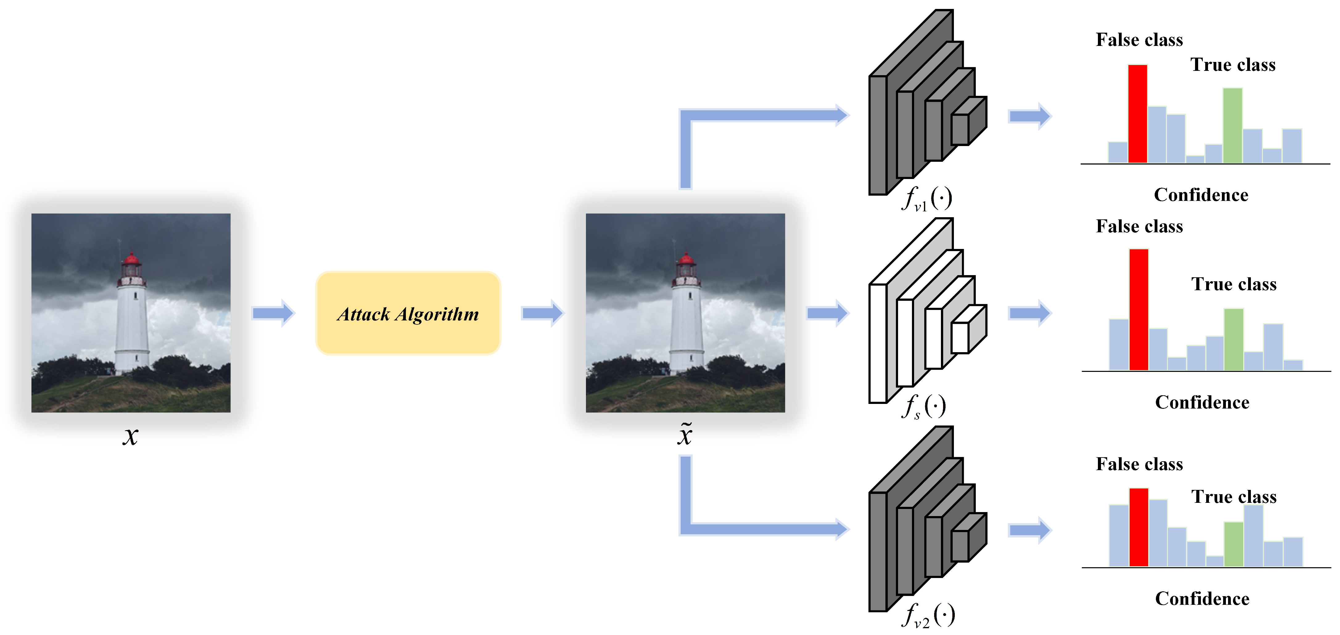
2.2. Transferability of Adversarial Examples

We consider an extreme situation where attackers have no access to any feedback from victim models, in which existing white-box and black-box attacks are unable to craft adversarial examples. In this case, attackers can utilize the transferability of adversarial examples to attack models. Specifically, the extensive experiments in [18] have demonstrated that adversarial examples can transfer among models, even if they have different architectures or are trained on different training sets, so long as they are trained to perform the same task. Details about the transferability are shown in Figure 1.
As shown in Figure 1, for an image classification task, we have trained three recognition models. Suppose that only the surrogate model f s ( · ) is a white-box model, and victim models f v 1 ( · ) , f v 2 ( · ) are black-box models. Undoubtedly, given an sample x, attackers can craft an adversarial example x ˜ to fool f s ( · ) through attack algorithms. Meanwhile, given the transferability of adversarial examples, x ˜ can also fool f v 1 ( · ) and f v 2 ( · ) successfully. However, the transferability generated by existing algorithms is very weak, so this paper is dedicated to crafting highly transferable adversarial examples.

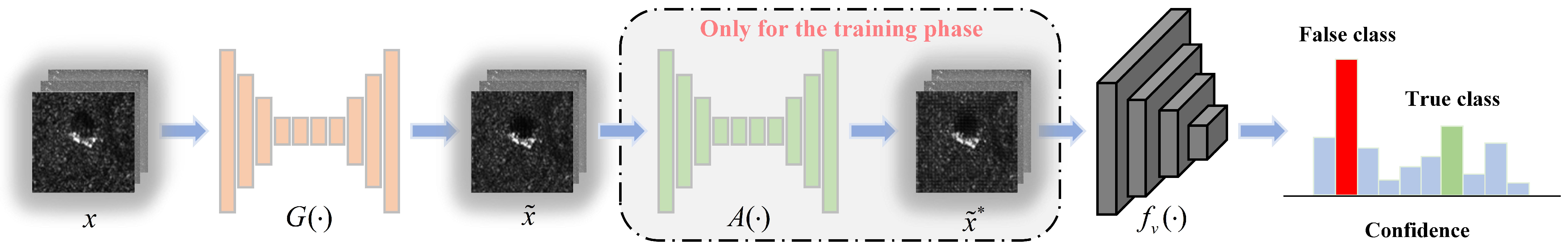
3. The Proposed Transferable Adversarial Network (TAN)

In this paper, the proposed Transferable Adversarial Network (TAN) utilizes the encoder–decoder model and data augmentation technology to improve the transferability and real-time performance of adversarial examples. The framework of our network is shown in Figure 2. As we can see, compared to traditional iterative methods, TAN introduces a generator G ( · ) to learn the one-step forward mapping from the clean sample x to the adversarial example x ˜ , thus enabling real-time attacks. Meanwhile, to improve the transferability of x ˜ , we simultaneously trained an attenuator A ( · ) to capture the most harmful deformations, which are supposed to weaken the effectiveness of x ˜ while still preserving the semantic meaning of x. We argue that if x ˜ is robust to the deformations produced by A ( · ) , i.e., x ˜ * remains effective to DNN models, then x ˜ is capable of transferring to the black-box victim model f v ( · ) . In other words, we achieve real-time transferable adversarial attacks through a two-player game between G ( · ) and A ( · ) . This chapter will introduce our method in detail.

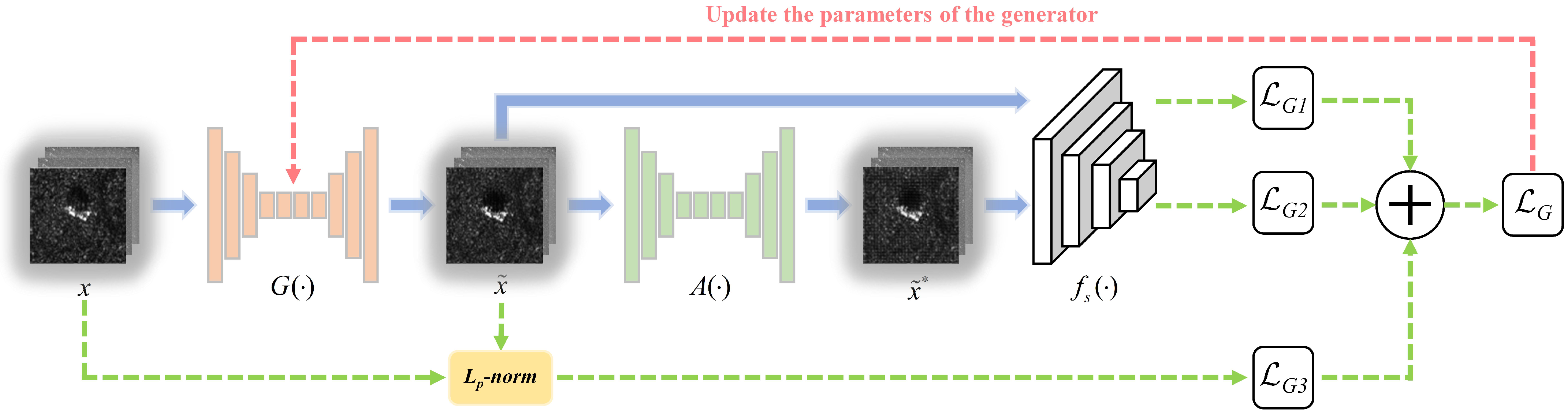
3.1. Training Process of the Generator

For easy understanding, Figure 3 shows the detailed training process of the generator. Note that a white-box model is selected as the surrogate model f s ( · ) during the training phase.
As we can see, given a clean sample x, the generator G ( · ) crafts the adversarial example x ˜ through a one-step forward mapping, as follows:
x ˜ = G ( x )
Meanwhile, the attenuator A ( · ) takes x ˜ as input and outputs the attenuated adversarial example x ˜ * :
x ˜ * = A ( x ˜ )
Since x ˜ has to fool f s ( · ) with a minor perturbation, and x ˜ * needs to remain effective against f s ( · ) , the loss function of G ( · ) consists of three parts. Next, we will give the generator loss L G of non-targeted and targeted attacks, respectively.
For the non-targeted attack: First, according to (2), x ˜ is to minimize the classification accuracy of f s ( · ) , which means that it has to decrease the confidence of being recognized as the true class C t r , i.e., to increase the confidence of being identified as others. Thus, the first part of L G can be expressed as:
L G 1 ( f s ( x ˜ ) , C t r ) = log i C t r exp ( f s ( x ˜ ) i ) i exp ( f s ( x ˜ ) i ) = log 1 exp ( f s ( x ˜ ) C t r ) i exp ( f s ( x ˜ ) i )
Second, to improve the transferability of x ˜ , we expect that x ˜ * remains effective to f s ( · ) , so the second part of L G can be derived as:
L G 2 ( f s ( x ˜ * ) , C t r ) = log i C t r exp ( f s ( x ˜ * ) i ) i exp ( f s ( x ˜ * ) i ) = log 1 exp ( f s ( x ˜ * ) C t r ) i exp ( f s ( x ˜ * ) i )
Finally, the last part of L G is used to limit the perturbation magnitude. We introduce the traditional L p -norm to measure the degree of image distortion as follows:
L G 3 ( x , x ˜ ) = x ˜ x p = ( i Δ x i p ) 1 p
In summary, we apply the linear weighted sum method to balance the relationship among L G 1 , L G 2 , and L G 3 . As such, the complete generator loss for the non-targeted attack can be represented as:
L G = ω G 1 · L G 1 ( f s ( x ˜ ) , C t r ) + ω G 2 · L G 2 ( f s ( x ˜ * ) , C t r ) + ω G 3 · L G 3 ( x , x ˜ )
where ω G 1 + ω G 2 + ω G 3 = 1 . ω G 1 , ω G 2 , ω G 3 [ 0 , 1 ] are the weight coefficients of L G 1 , L G 2 , and L G 3 , respectively. The weight coefficients represent the relative importance of each loss term during the training process. A larger weight implies that the corresponding loss will decrease more rapidly and significantly, allowing attackers to adjust the parameters flexibly according to their actual needs.
For the targeted attack: According to (3), x ˜ is to maximize the probability of being recognized as the target class C t a , i.e., to increase the confidence of C t a . Thus, L G 1 here can be expressed as:
L G 1 ( f s ( x ˜ ) , C t a ) = log exp ( f s ( x ˜ ) C t a ) i exp ( f s ( x ˜ ) i )
To maintain the effectiveness of x ˜ * against f s ( · ) , L G 2 here is derived as:
L G 2 ( f s ( x ˜ * ) , C t a ) = log exp ( f s ( x ˜ * ) C t a ) i exp ( f s ( x ˜ * ) i )
The perturbation magnitude is still limited by the L G 3 shown in (8). Therefore, the complete generator loss for the targeted attack can be represented as:
L G = ω G 1 · L G 1 ( f s ( x ˜ ) , C t a ) + ω G 2 · L G 2 ( f s ( x ˜ * ) , C t a ) + ω G 3 · L G 3 ( x , x ˜ )

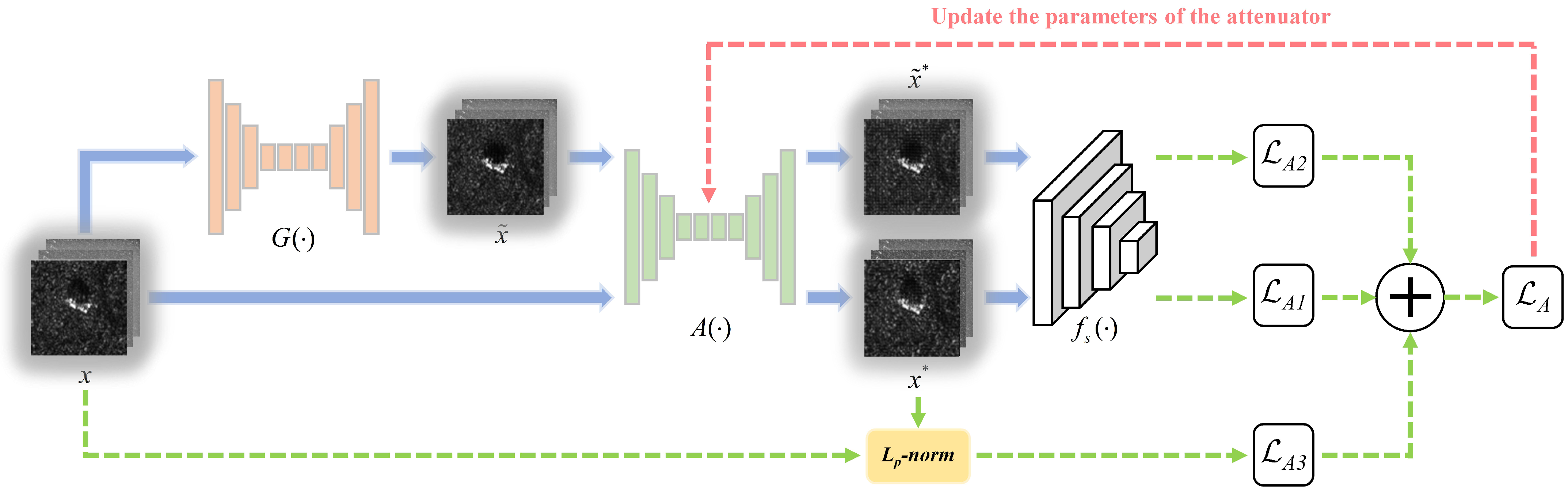
3.2. Training Process of the Attenuator

According to Figure 2, during the training phase of TAN, an attenuator A ( · ) was introduced to weaken the effectiveness of x ˜ while still preserving the semantic meaning of x. We show the detailed training process of A ( · ) in Figure 4.
As we can see, the attenuator loss L A also consists of three parts. First, to preserve the semantic meaning of x, f s ( · ) has to keep a basic classification accuracy on the following attenuated sample x * :
x * = A ( x )
It means that the first part of L A should increase the confidence of x * being recognized as the true class C t r , as follows:
L A 1 ( f s ( x * ) , C t r ) = log exp ( f s ( x * ) C t r ) i exp ( f s ( x * ) i )
Meanwhile, to weaken the effectiveness of x ˜ , A ( · ) also need to improve the confidence of the attenuated adversarial example x ˜ * being identified as C t r , so the second part of L A can be expressed as:
L A 2 ( f s ( x ˜ * ) , C t r ) = log exp ( f s ( x ˜ * ) C t r ) i exp ( f s ( x ˜ * ) i )
Finally, to avoid excessive image distortion caused by A ( · ) , the third part of L A is used to limit the deformation magnitude, which can be expressed by the traditional L p -norm, as follows:
L A 3 ( x , x * ) = x * x p = ( i Δ x i p ) 1 p
As with the generator loss, we utilize the linear weighted sum method to derive the complete attenuator loss as follows:
L A = ω A 1 · L A 1 ( f s ( x * ) , C t r ) + ω A 2 · L A 2 ( f s ( x ˜ * ) , C t r ) + ω A 3 · L A 3 ( x , x * )
where ω A 1 + ω A 2 + ω A 3 = 1 . ω A 1 , ω A 2 , ω A 3 [ 0 , 1 ] are the weight coefficients of L A 1 , L A 2 , and L A 3 , respectively.

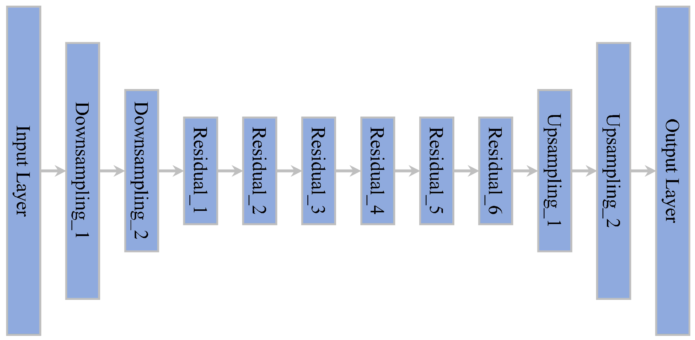
3.3. Network Structure of the Generator and Attenuator

According to Section 3.1 and  Section 3.2, the generator and attenuator are essentially two encoder–decoder models, so the choice of a suitable model structure is necessary. We mainly consider two factors. First, as the size of original samples and adversarial examples should be the same, the model has to keep the input and output sizes identical. Second, to prevent our network from overfitting while saving computational resources, a lightweight model will be a better choice. In summary, we applied ResNet Generator proposed in [29] as the encoder–decoder model of TAN. The structure of ResNet Generator is shown in Figure 5.
As we can see, ResNet Generator mainly consists of downsampling, residual, and upsampling modules. For a visual understanding, given an input data of size 1 × 128 × 128 , the input and output sizes of each module are listed in Table 1.
Obviously, the input and output sizes of ResNet Generator are the same. Meanwhile, to ensure the validity of the generated data, we added a t a n h function after the output module, which restricts the generated data to the interval [ 0 , 1 ] . The total number of parameters in ResNet Generator has been calculated to be approximately 7.83 M , which is a fairly lightweight network. For more details, please refer to the literature [29].

3.4. Complete Training Process of TAN

As we described earlier, TAN improves the transferability of adversarial examples through a two-player game between the generator and attenuator, which is quite similar to the working principle of generative adversarial networks (GAN) [30]. Therefore, we also adopted an alternating training scheme to train our network. Specifically, given the dataset X and batch size S, we first randomly divided X into M batches { b 1 , b 2 , , b M } at the beginning of each training iteration. Second, we set a training ratio R N * , which means that TAN trains the generator R times and then trains the attenuator once, i.e., once per batch for the former and only once per R batch for the latter. In this way, we can prevent the attenuator from being so strong that the generator cannot be optimized. Meanwhile, to shorten training time, we set an early stop condition E s c so that training can be ended early when certain indicators meet the condition. Note that the generator and attenuator are trained alternately, i.e., the attenuator’s parameters are fixed when the generator is trained, and vice versa. More details of the complete training process for TAN are shown in Algorithm 1.
Algorithm 1:Transferable Adversarial Network Training
Input: 
Dataset X ; batch size S; surrogate model f s ; target class C t a ; training loss function L G of the generator; training loss function L A of the attenuator; training iteration number T; learning rate η ; training ratio R of the generator and attenuator; early stop condition E s c .
Output: 
The parameter θ G of the well-trained generator.
1:
Randomly initialize θ G and θ A
2:
for t = 1 to T do
3:
    According to S, randomly divide X into M batches { b 1 , b 2 , , b M }
4:
    for  m = 1 to M do
5:
        Calculate L G ( θ G , θ A , f s , b m , C t a )
6:
        Update θ G = θ G η · θ G L G
7:
        if  m % R = = 0  then
8:
           Calculate L A ( θ G , θ A , f s , b m )
9:
           Update θ A = θ A η · θ A L A
10:
        else
11:
            θ A = θ A
12:
        end if
13:
    end for
14:
    if  E s c = = T r u e  then
15:
        Break
16:
    else
17:
        Continue
18:
    end if
19:
end for

4. Experiments

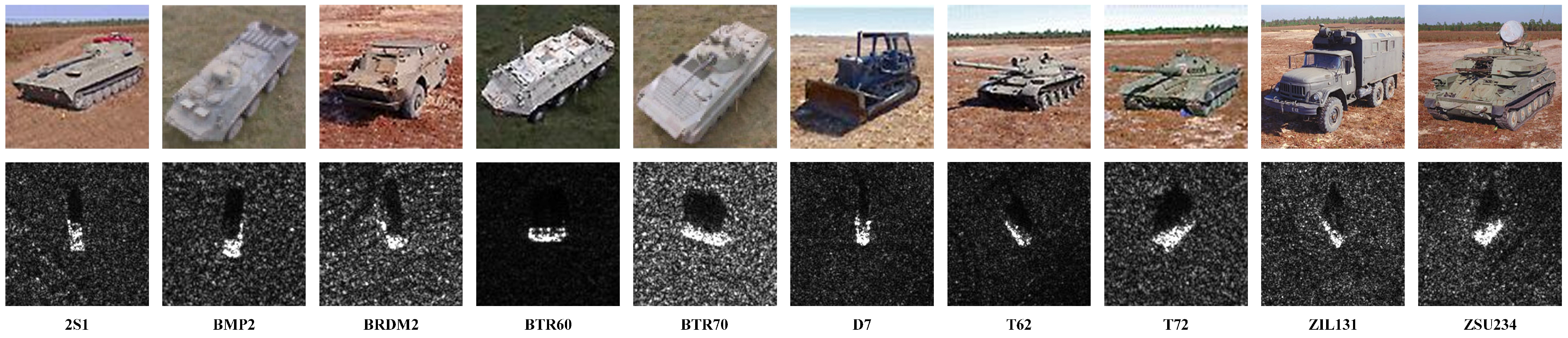
4.1. Data Descriptions

To date, there is no publicly available dataset for UAV SAR-ATR, thus this paper experiments on the most authoritative SAR-ATR dataset, i.e., the moving and stationary target acquisition and recognition (MSTAR) dataset [31]. MSTAR is collected by a high-resolution spotlight SAR and published by the U.S. Defense Advanced Research Projects Agency (DARPA) in 1996, which contains SAR images of Soviet military vehicle targets at different azimuth and depression angles. In standard operating conditions (SOC), MSTAR includes ten classes of targets, such as self-propelled howitzers (2S1); infantry fighting vehicles (BMP2); armored reconnaissance vehicles (BRDM2); wheeled armored transport vehicles (BTR60, BTR70); bulldozers (D7); main battle tanks (T62, T72); cargo trucks (ZIL131); and self-propelled artillery (ZSU234). The training dataset contains 2747 images collected at a depression angle of 17 , and the testing dataset contains 2426 images captured at a depression angle of 15 . More details about the dataset are given in Table 2, and Figure 6 shows the optical images and corresponding SAR images of each class.

4.2. Implementation Details

The proposed method is evaluated on the following six common DNN models: DenseNet121 [32], GoogLeNet [33], InceptionV3 [34], Mobilenet [35], ResNet50 [36], and Shufflenet [37]. In terms of data preprocessing, we resized all the images in MSTAR to 128 × 128 and uniformly sample 10 % of training data to form the validation dataset. During the training phase of recognition models, the training epoch and batch size were set to 100 and 32, respectively. During the training phase of TAN, to minimize the MSE between adversarial examples and original samples, we adopted the L 2 -norm to evaluate the image distortion caused by adversarial perturbations. Meanwhile, for better attack performance, the hyperparameters of TAN are fine-tuned through numerous experiments, and the following set of parameters is eventually determined to best meet our requirements. Specifically, we set the generator loss weights [ ω G 1 , ω G 2 , ω G 3 ] to [ 0.25 , 0.25 , 0.5 ] , the attenuator loss weights [ ω A 1 , ω A 2 , ω A 3 ] to [ 0.25 , 0.25 , 0.5 ] , the training ratio to 3, the training epoch to 50, and the batch size to 8. Due to the adversarial process involved in TAN, training can be challenging to converge. As such, we employed Adam [38], a more computationally efficient optimizer, to accelerate model convergence, which also performs better in solving non-stationary objective and sparse gradient problems. The learning rate is set to 0.001 . When evaluating the transferability, we first crafted adversarial examples for each surrogate model and then assessed the transferability by testing the recognition results of victim models on corresponding adversarial examples. Detailed experiments will be given later.
Furthermore, the following six attack algorithms from the Torchattacks [39] toolbox were introduced as baseline methods for comparison with TAN: MIFGSM [19], DIFGSM [21], NIFGSM [20], SINIFGSM [20], VMIFGSM [22], and VNIFGSM [22]. All codes were written in Pytorch, and the experimental environment consisted of Windows 10 with an NVIDIA GeForce RTX 2080 Ti GPU and a 3.6 GHz Intel Core i9-9900K CPU.

4.3. Evaluation Metrics

We mainly consider two factors to comprehensively evaluate the performance of adversarial attacks: the effectiveness and stealthiness, which are directly related to the classification accuracy A c c ˜ of victim models on adversarial examples and the norm value L ˜ p of adversarial perturbations, respectively. For the A c c ˜ metric, the formula is as follows:
A c c ˜ = 1 N n = 1 N D ( arg max i ( f v ( x ˜ n ) i ) = = C t r ) for the non - targeted attack 1 K × N C t a = 1 K n = 1 N D ( arg max i ( f v ( x ˜ n ) i ) = = C t a ) for the targeted attack
where C t r and C t a represent the true and target classes of the input data, K is the number of target classes, and D ( · ) is a discriminant function. In the non-targeted attack, the A c c ˜ metric reflects the probability that the victim model f v ( · ) identifies the adversarial example x ˜ n as C t r , while in the targeted attack it indicates the probability that f v ( · ) recognizes x ˜ n as C t a . Obviously, in the non-targeted attack, the lower the A c c ˜ metric, the better the attack. Conversely, in the targeted attack, a higher A c c ˜ metric represents f v ( · ) is more likely to recognize x ˜ n as C t a , and thus the attack is more effective. In conclusion, the effectiveness of non-targeted attacks is inversely proportional to the A c c ˜ metric, and the effectiveness of targeted attacks is proportional to this metric. Additionally, there are other three similar indicators, A c c , A c c * , and A c c ˜ * , that represent the classification accuracy of f v ( · ) for the original sample x n , the attenuated sample x n * , and the attenuated adversarial example x ˜ n * , respectively. Note that whether it is a non-targeted or targeted attack, A c c * always represents the accuracy with which f v ( · ) identifies x n * as C t r , while the other three accuracy indicators need to be calculated via (18) based on the attack mode. In particular, A c c ˜ * represents the recognition result of f v ( · ) on x ˜ n * , which indirectly reflects the strength of the transferability possessed by x ˜ n .
Meanwhile, we applied the following L p -norm values to measure the attack stealthiness:
L ˜ p = 1 N n = 1 N x ˜ n x n p for the generator L p * = 1 N n = 1 N x n * x n p for the attenuator
where L ˜ p and L p * represent the image distortion caused by the generator and attenuator, respectively. In our experiments, the L p -norm defaults to L 2 -norm. In summary, we can set the early stop condition E s c mentioned in Section 3.4 with the above indicators, as follows:
E s c = A c c ˜ 0.05 , A c c * 0.9 , A c c ˜ * 0.1 , L ˜ 2 4 , L 2 * 4 for the non - targeted attack A c c ˜ 0.95 , A c c * 0.9 , A c c ˜ * 0.9 , L ˜ 2 4 , L 2 * 4 for the targeted attack
Furthermore, to evaluate the real-time performance of adversarial attacks, we introduced the T c metric to denote the time cost of generating a single adversarial example, as follows:
T c = T i m e N
where T i m e is the total time consumed to generate N adversarial examples.

4.4. DNN-Based SAR-ATR Models

A well-trained recognition model is a prerequisite for effective adversarial attacks, so we have trained six SAR-ATR models on the MSTAR dataset: DenseNet121, GoogLeNet, InceptionV3, Mobilenet, ResNet50, and Shufflenet. All of them achieve outstanding recognition performance, with the classification accuracy of 98.72 % , 98.06 % , 96.17 % , 96.91 % , 97.98 % , and 96.66 % on the testing dataset, respectively. In addition, we show the confusion matrix of each model in Figure 7.

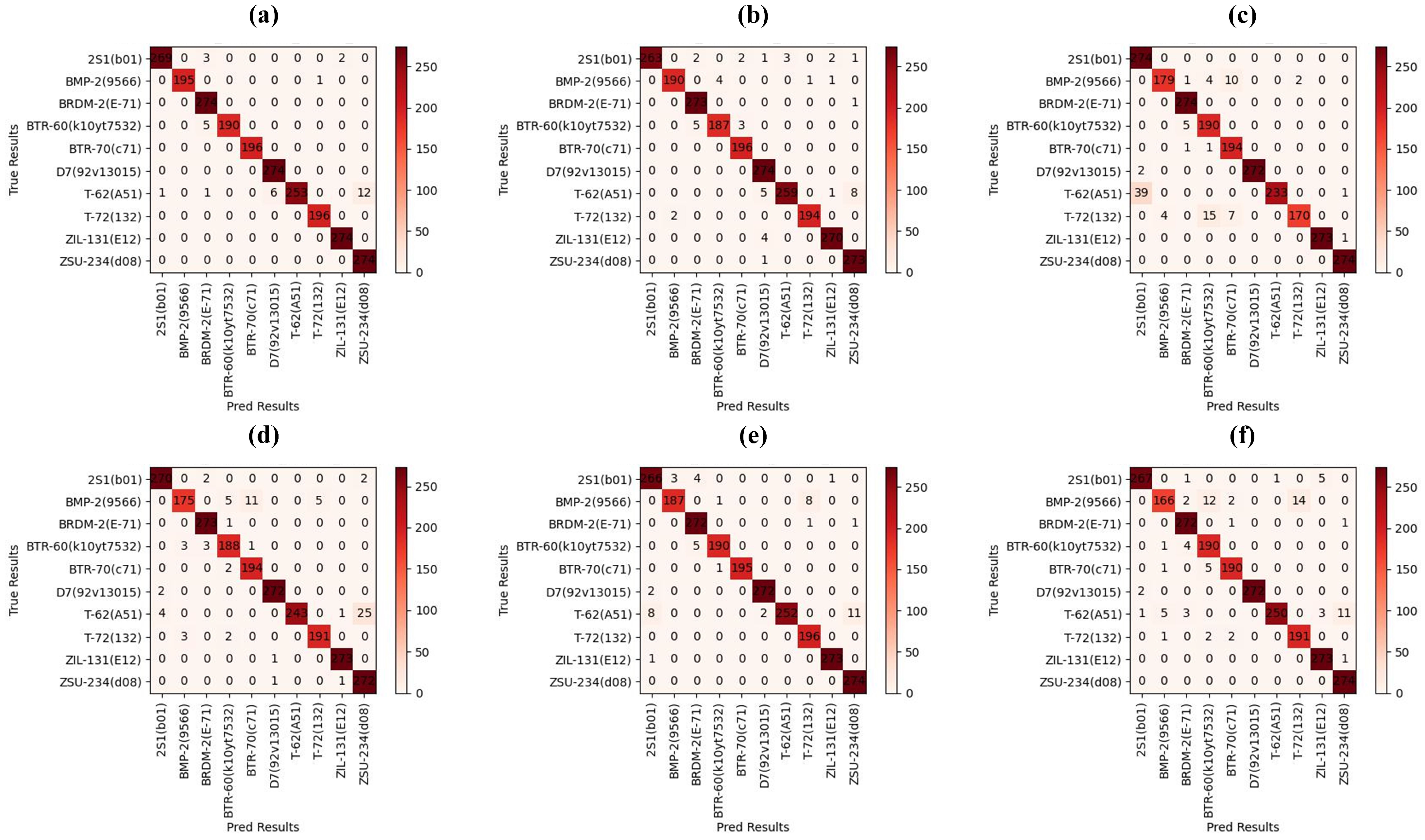
4.5. Comparison of Attack Performance

In this section, we first evaluated the attack performance of the proposed method against DNN-based SAR-ATR models on the MSTAR dataset. Specifically, during the training phase of TAN, we took each network as the surrogate model in turn and assessed the recognition results of corresponding models on the outputs of TAN at each stage. The results of non-targeted and targeted attacks are detailed in Table 3 and Table 4, respectively.
In non-targeted attacks, the A c c metric of each model on the MSTAR dataset exceeds 95 % . However, after the non-targeted attack, the classification accuracy of all models on the generated adversarial examples, i.e., the A c c ˜ metric, is below 5 % , and the L ˜ 2 indicator is less than 3.7 . It means that adversarial examples deteriorate the recognition performance of models rapidly through minor adversarial perturbations. Meanwhile, during the training phase of TAN, we evaluate the performance of the attenuator. According to the A c c ˜ * metric, the attenuator leads to an average improvement of about 25 % in the classification accuracy of models on adversarial examples, that is, it indeed weakens the effectiveness of adversarial examples. We also should pay attention to the metrics A c c * and L 2 * , i.e., the recognition accuracy of models on the attenuated samples, and the deformation distortion caused by the attenuator. The fact is that the A c c * indicator of each model exceeds 80 % , and the average value of the L 2 * metric is about 4. It means that the attenuator retains most semantic information of original samples without causing excessive deformation distortion, which is in line with our requirements.
In targeted attacks, the A c c metric represents the probability that models identify original samples as target classes, so it can reflect the dataset distribution, i.e., each category accounts for about 10 % of the total dataset. After the targeted attack, the probability of each model recognizing adversarial examples as target classes, i.e., the A c c ˜ metric, is over 97 % , and the L ˜ 2 indicator shows that the image distortion caused by adversarial perturbations is less than 3.5 . It means that the adversarial examples crafted by the generator can induce models to output specified results with high probability through minor perturbations. As with the non-targeted attack, we evaluate the performance of the attenuator. The A c c ˜ * metric shows that the attenuator results in an average decrease of about 17 % in the probability of adversarial examples being identified as target classes. Meanwhile, the A c c * metric of each model exceeds 85 % , and the average value of the L 2 * indicator is about 3.7 . That is, the attenuator weakens the effectiveness of adversarial examples through slight deformations, while preserving the semantic meaning of original samples well.
In summary, for both non-targeted and targeted attacks, the adversarial examples crafted by the generator can fool models with high success rates, and the attenuator is able to weaken the effectiveness of adversarial examples with slight deformations while retaining the semantic meaning of original samples. Moreover, we ensure that the generator always outperforms the attenuator by adjusting the training ratio between the two models. To visualize the attack results of TAN, we took ResNet50 as the surrogate model and display the outputs of TAN at each stage in Figure 8.
Finally, we compared the non-targeted and targeted attack performance of different methods against DNN-based SAR-ATR models on the MSTAR dataset, as detailed in Table 5. Obviously, for the same image distortion, the attack effectiveness of the proposed method against a single model may not be the best. Nevertheless, we focused more on the transferability of adversarial examples, which will be the main topic of the following section.

4.6. Comparison of Transferability

In this section, we evaluated the transferability of adversarial examples among DNN-based SAR-ATR models on the MSTAR dataset. Specifically, we first took each network as the surrogate model in turn and crafted adversarial examples for them, respectively. Then, we assessed the transferability by testing the recognition results of victim models on corresponding adversarial examples. The transferability in non-targeted and targeted attacks are shown in Table 6 and Table 7, respectively.
In non-targeted attacks, when the proposed method sequentially takes DenseNet121, GoogLeNet, InceptionV3, Mobilenet, ResNet50, and Shufflenet as the surrogate model, the highest recognition accuracy of victim models on the generated adversarial examples are 12.90 % , 26.88 % , 23.45 % , 18.59 % , 11.01 % , and 23.54 % , respectively. Equivalently, the highest recognition accuracy of victim models on the adversarial examples produced by baseline methods are 36.11 % , 44.44 % , 56.06 % , 65.99 % , 33.84 % , and 68.51 % , respectively. Meanwhile, for each surrogate model, victim models always have the lowest recognition accuracy on the adversarial examples crafted by our approach. Obviously, compared with baseline methods, the proposed method slightly sacrifices the performance on attacking surrogate models, but achieves state-of-the-art transferability among victim models in non-targeted attacks. Detailed results are shown in Table 6.
In targeted attacks, the proposed method still takes DenseNet121, GoogLeNet, InceptionV3, Mobilenet, ResNet50, and Shufflenet as the surrogate model in turn, and the minimum probability that victim models identify the generated adversarial examples as target classes are 52.39 % , 55.02 % , 54.57 % , 57.66 % , 66.26 % , and 47.78 % , respectively. Correspondingly, the minimum probability that victim models recognize the adversarial examples produced by baseline methods as target classes are 22.18 % , 19.63 % , 19.49 % , 15.52 % , 19.36 % , and 13.06 % , respectively. Moreover, for each surrogate model, victim models always identify the adversarial examples crafted by our approach as target classes with the maximum probability. Thus, the proposed method also achieves state-of-the-art transferability among victim models in targeted attacks. Detailed results are shown in Table 7.
In conclusion, for both non-targeted and targeted attacks, our approach generates adversarial examples with the strongest transferability. In other words, it performs better on exploring the common vulnerability of DNN models. We attribute this to the adversarial training between the generator and attenuator. Figuratively speaking, it is because of the attenuator constantly creating obstacles for the generator that the attack capability of the generator is continuously enhanced and completed.

4.7. Comparison of Real-Time Performance

According to (4), compared to traditional iterative methods, the generator in our approach is capable of one-step mapping original samples to adversarial examples. It acts like a function that takes inputs and outputs results based on the mapping relationship. To evaluate the real-time performance of adversarial attacks, we compared the time cost of generating a single adversarial example through different attack algorithms. The time consumption of non-targeted and targeted attacks is shown in Table 8 and Table 9, respectively.
As we can see, there is almost no difference in the time cost of crafting a single adversarial example in non-targeted and targeted attacks. Meanwhile, for all the victim models, the time cost of generating a single adversarial example through our method is stable around 2 ms. As for baseline methods, it depends on the complexity of victim models, the more complex the model, the longer the time cost. However, even for the simplest victim model, the minimum time cost of baseline methods is about 4.5 ms, consuming twice as much time as our approach. Thus, there is no doubt that the proposed method achieves the most superior and stable real-time performance.

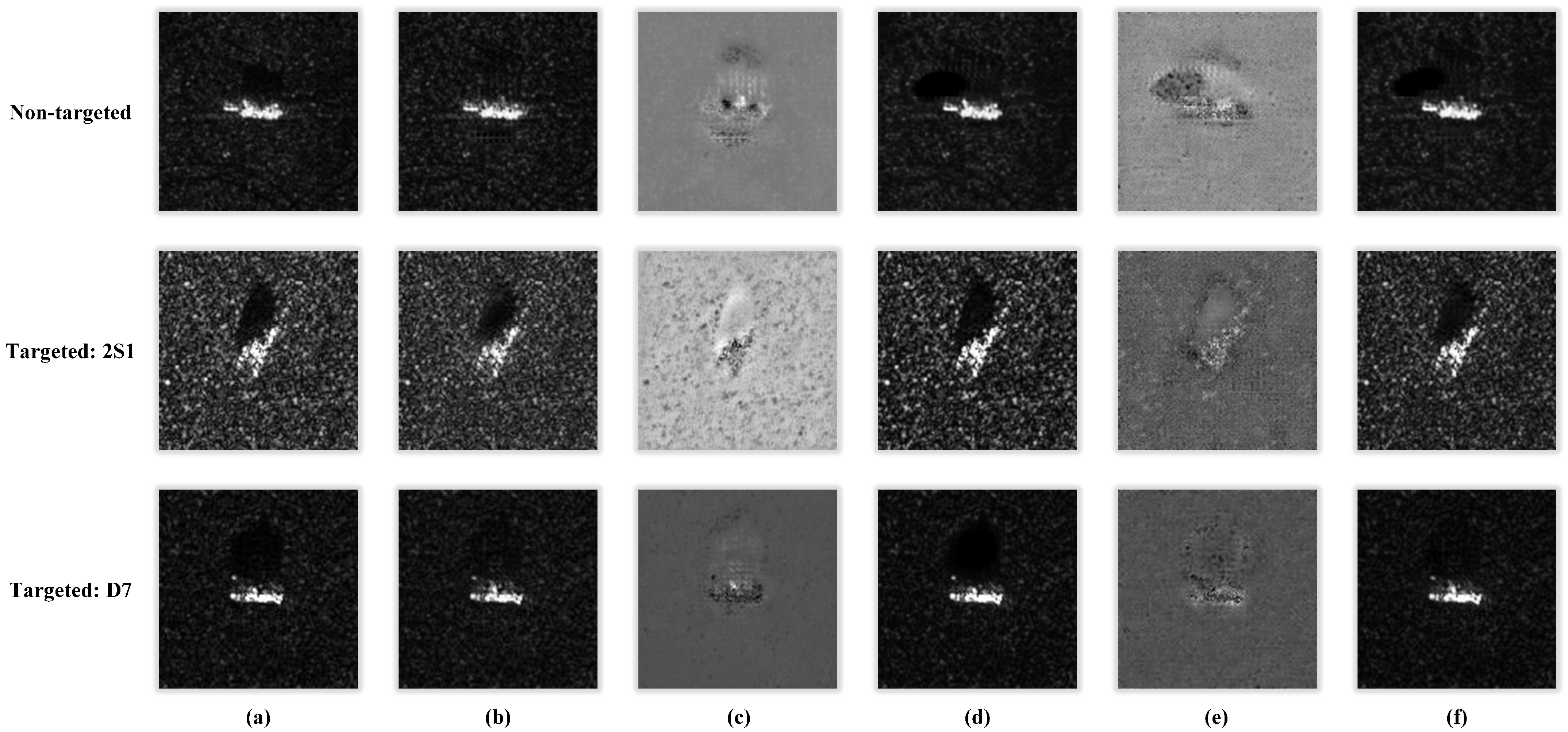
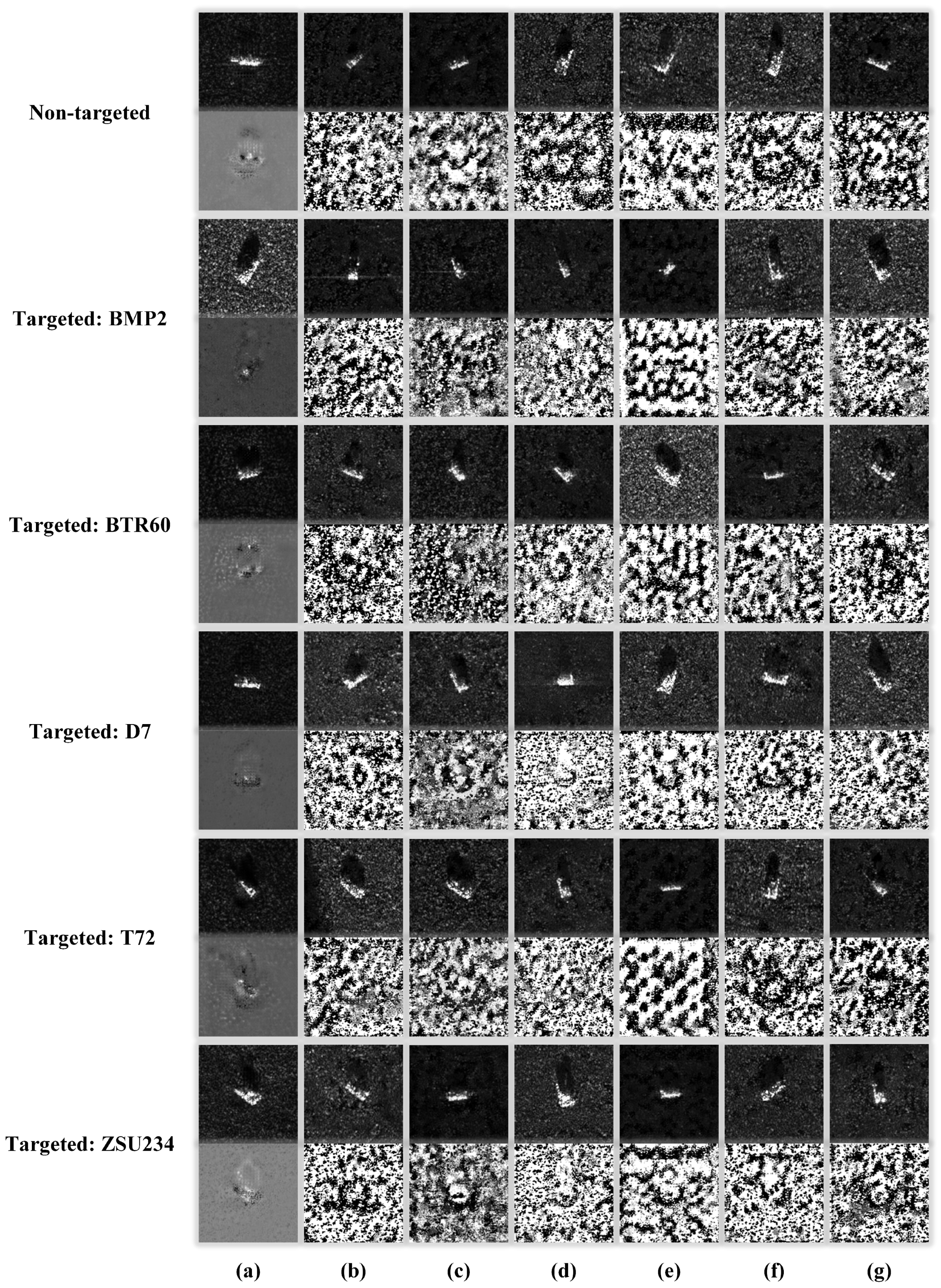
4.8. Visualization of Adversarial Examples

In this section, we took ResNet50 as the surrogate model and visualized the adversarial examples crafted by different methods in Figure 9. Obviously, the adversarial perturbations generated by our method are continuous, and mainly focus on the target region of SAR images. In contrast, the perturbations produced by baseline methods are quite discrete, and almost cover the global area of SAR images. First, from the perspective of feature extraction, since the features that have a greater impact on recognition results are mainly concentrated in the target region rather than the background clutter area, a focused disruption of key features is certainly a more efficient attack strategy. Second, from the perspective of physical feasibility, the fewer pixels modified in adversarial examples, the smaller range perturbed in reality, so localized perturbations are more feasible than global ones. In summary, the proposed method improves the efficiency and feasibility of adversarial attacks by focusing perturbations on the target region of SAR images.

5. Discussions

So far, the proposed method has been proven to be effective for SAR images. Further studies should verify its effectiveness in other fields, such as optical [40,41], infrared [42,43], and synthetic aperture sonar (SAS) [44,45,46,47] images, etc. Although different imaging principles lead to huge differences in the resolution, dimension, and target type of images, we argue that TAN can be well-suitable to these fields. The reason is that adversarial examples essentially attack the inherent vulnerability of DNN models, independent of the input data. However, the non-negligible challenge is how to realize these adversarial examples in the real world. Specifically, the physical implementation depends on the imaging principle, e.g., crafting adversarial patches against optical cameras, changing temperature against infrared devices, and emitting acoustic signals against SAS, etc. This is a worthwhile topic in the future.

6. Conclusions

This paper proposed a transferable adversarial network (TAN) to attack DNN-based SAR-ATR models, with the benefit that the transferability and the real-time performance of adversarial examples is significantly improved, which is of great significance for real-world black-box attacks. In the proposed method, we simultaneously trained two encoder–decoder models: a generator that learns the one-step forward mapping from original data to adversarial examples, and an attenuator that captures the most harmful deformations to malicious samples. It is motivated by enabling real-time attacks by one-step mapping original data to adversarial examples, and enhancing the transferability through a two-player game between the generator and attenuator. Experimental results demonstrated that our approach achieves state-of-the-art transferability with acceptable adversarial perturbations and minimum time costs compared to existing attack methods, making real-time black-box attacks without any prior knowledge a reality. Potential future work could consider attacking DNN-based SAR-ATR models under small sample conditions. In addition to improving the performance of attack algorithms, it makes sense to implement adversarial examples in the real world.

Author Contributions

Conceptualization, M.D. (Meng Du) and D.B.; methodology, M.D. (Meng Du); software, M.D. (Meng Du); validation, D.B., Y.S., B.S. and Z.W.; formal analysis, D.B. and M.D. (Mingyang Du); investigation, M.D. (Mingyang Du); resources, D.B.; data curation, M.D. (Meng Du); writing—original draft preparation, M.D. (Meng Du); writing—review and editing, M.D. (Meng Du), L.L. and D.B.; visualization, M.D. (Meng Du); supervision, D.B.; project administration, D.B.; funding acquisition, D.B. All authors have read and agreed to the published version of the manuscript.

Funding

This work was supported by the National Natural Science Foundation of China under Grant 62071476.

Institutional Review Board Statement

The study does not involve humans or animals.

Informed Consent Statement

The study does not involve humans.

Data Availability Statement

The experiments in this paper use public datasets, so no data are reported in this work.

Conflicts of Interest

The authors declare that they have no conflict of interest to report regarding the present study.

References

  1. Li, D.; Kuai, Y.; Wen, G.; Liu, L. Robust Visual Tracking via Collaborative and Reinforced Convolutional Feature Learning. In Proceedings of the IEEE/CVF Conference on Computer Vision and Pattern Recognition Workshops, Long Beach, CA, USA, 15–19 June 2019. [Google Scholar] [CrossRef]
  2. Kuai, Y.; Wen, G.; Li, D. Masked and dynamic Siamese network for robust visual tracking. Inf. Sci. 2019, 503, 169–182. [Google Scholar] [CrossRef]
  3. Cong, R.; Yang, N.; Li, C.; Fu, H.; Zhao, Y.; Huang, Q.; Kwong, S. Global-and-local collaborative learning for co-salient object detection. IEEE Trans. Cybern. 2022, 53, 1920–1931. [Google Scholar] [CrossRef] [PubMed]
  4. Tang, J.; Xiang, D.; Zhang, F.; Ma, F.; Zhou, Y.; Li, H. Incremental SAR Automatic Target Recognition With Error Correction and High Plasticity. IEEE J. Sel. Top. Appl. Earth Obs. Remote Sens. 2022, 15, 1327–1339. [Google Scholar] [CrossRef]
  5. Wang, L.; Yang, X.; Tan, H.; Bai, X.; Zhou, F. Few-Shot Class-Incremental SAR Target Recognition Based on Hierarchical Embedding and Incremental Evolutionary Network. IEEE Trans. Geosci. Remote Sens. 2023, 2023, 3248040. [Google Scholar] [CrossRef]
  6. Kwak, Y.; Song, W.J.; Kim, S.E. Speckle-Noise-Invariant Convolutional Neural Network for SAR Target Recognition. IEEE Geosci. Remote Sens. Lett. 2019, 16, 549–553. [Google Scholar] [CrossRef]
  7. Du, C.; Chen, B.; Xu, B.; Guo, D.; Liu, H. Factorized discriminative conditional variational auto-encoder for radar HRRP target recognition. Signal Process. 2019, 158, 176–189. [Google Scholar] [CrossRef]
  8. Vint, D.; Anderson, M.; Yang, Y.; Ilioudis, C.; Di Caterina, G.; Clemente, C. Automatic Target Recognition for Low Resolution Foliage Penetrating SAR Images Using CNNs and GANs. Remote Sens. 2021, 13, 596. [Google Scholar] [CrossRef]
  9. Huang, T.; Zhang, Q.; Liu, J.; Hou, R.; Wang, X.; Li, Y. Adversarial attacks on deep-learning-based SAR image target recognition. J. Netw. Comput. Appl. 2020, 162, 102632. [Google Scholar] [CrossRef]
  10. Szegedy, C.; Zaremba, W.; Sutskever, I.; Bruna, J.; Erhan, D.; Goodfellow, I.; Fergus, R. Intriguing properties of neural networks. arXiv 2013, arXiv:1312.6199. [Google Scholar]
  11. Goodfellow, I.J.; Shlens, J.; Szegedy, C. Explaining and harnessing adversarial examples. arXiv 2014, arXiv:1412.6572. [Google Scholar] [CrossRef]
  12. Kurakin, A.; Goodfellow, I.J.; Bengio, S. Adversarial examples in the physical world. In Artificial Intelligence Safety and Security; Chapman and Hall/CRC: London, UK, 2018; pp. 99–112. [Google Scholar]
  13. Moosavi-Dezfooli, S.M.; Fawzi, A.; Frossard, P. Deepfool: A simple and accurate method to fool deep neural networks. In Proceedings of the IEEE Conference on Computer Vision and Pattern Recognition, Las Vegas, NV, USA, 26 June–1 July 2016; pp. 2574–2582. [Google Scholar] [CrossRef] [Green Version]
  14. Papernot, N.; McDaniel, P.; Jha, S.; Fredrikson, M.; Celik, Z.B.; Swami, A. The limitations of deep learning in adversarial settings. In Proceedings of the 2016 IEEE European Symposium on Security and Privacy (EuroS&P), Saarbrücken, Germany, 21–24 March 2016; pp. 372–387. [Google Scholar] [CrossRef] [Green Version]
  15. Su, J.; Vargas, D.V.; Sakurai, K. One pixel attack for fooling deep neural networks. IEEE Trans. Evol. Comput. 2019, 23, 828–841. [Google Scholar] [CrossRef] [Green Version]
  16. Chen, P.Y.; Zhang, H.; Sharma, Y.; Yi, J.; Hsieh, C.J. Zoo: Zeroth order optimization based black-box attacks to deep neural networks without training substitute models. In Proceedings of the 10th ACM Workshop on Artificial Intelligence and Security, Dallas, TX, USA, 3 November 2017; pp. 15–26. [Google Scholar] [CrossRef] [Green Version]
  17. Chen, J.; Jordan, M.I.; Wainwright, M.J. Hopskipjumpattack: A query-efficient decision-based attack. In Proceedings of the 2020 IEEE Symposium on Security and Privacy (SP), San Francisco, CA, USA, 18–21 May 2020; pp. 1277–1294. [Google Scholar] [CrossRef]
  18. Papernot, N.; McDaniel, P.; Goodfellow, I. Transferability in machine learning: From phenomena to black-box attacks using adversarial samples. arXiv 2016, arXiv:1605.07277. [Google Scholar]
  19. Dong, Y.; Liao, F.; Pang, T.; Su, H.; Zhu, J.; Hu, X.; Li, J. Boosting adversarial attacks with momentum. In Proceedings of the IEEE Conference on Computer Vision and Pattern Recognition, Salt Lake City, UT, USA, 18–23 June 2018; pp. 9185–9193. [Google Scholar] [CrossRef] [Green Version]
  20. Lin, J.; Song, C.; He, K.; Wang, L.; Hopcroft, J.E. Nesterov accelerated gradient and scale invariance for adversarial attacks. arXiv 2019, arXiv:1908.06281. [Google Scholar]
  21. Xie, C.; Zhang, Z.; Zhou, Y.; Bai, S.; Wang, J.; Ren, Z.; Yuille, A.L. Improving transferability of adversarial examples with input diversity. In Proceedings of the IEEE/CVF Conference on Computer Vision and Pattern Recognition, Long Beach, CA, USA, 15–20 June 2019; pp. 2730–2739. [Google Scholar] [CrossRef]
  22. Wang, X.; He, K. Enhancing the transferability of adversarial attacks through variance tuning. In Proceedings of the IEEE/CVF Conference on Computer Vision and Pattern Recognition, Nashville, TN, USA, 20–25 June 2021; pp. 1924–1933. [Google Scholar] [CrossRef]
  23. Xu, Y.; Du, B.; Zhang, L. Assessing the threat of adversarial examples on deep neural networks for remote sensing scene classification: Attacks and defenses. IEEE Trans. Geosci. Remote Sens. 2020, 59, 1604–1617. [Google Scholar] [CrossRef]
  24. Xu, Y.; Ghamisi, P. Universal Adversarial Examples in Remote Sensing: Methodology and Benchmark. IEEE Trans. Geosci. Remote Sens. 2022, 60, 1–15. [Google Scholar] [CrossRef]
  25. Li, H.; Huang, H.; Chen, L.; Peng, J.; Huang, H.; Cui, Z.; Mei, X.; Wu, G. Adversarial examples for CNN-based SAR image classification: An experience study. IEEE J. Sel. Top. Appl. Earth Obs. Remote Sens. 2020, 14, 1333–1347. [Google Scholar] [CrossRef]
  26. Du, C.; Huo, C.; Zhang, L.; Chen, B.; Yuan, Y. Fast C&W: A Fast Adversarial Attack Algorithm to Fool SAR Target Recognition with Deep Convolutional Neural Networks. IEEE Geosci. Remote Sens. Lett. 2021, 19, 1–5. [Google Scholar] [CrossRef]
  27. Du, M.; Bi, D.; Du, M.; Xu, X.; Wu, Z. ULAN: A Universal Local Adversarial Network for SAR Target Recognition Based on Layer-Wise Relevance Propagation. Remote Sens. 2022, 15, 21. [Google Scholar] [CrossRef]
  28. Xia, W.; Liu, Z.; Li, Y. SAR-PeGA: A Generation Method of Adversarial Examples for SAR Image Target Recognition Network. IEEE Trans. Aerosp. Electron. Syst. 2022, 2022, 3206261. [Google Scholar] [CrossRef]
  29. Johnson, J.; Alahi, A.; Fei-Fei, L. Perceptual losses for real-time style transfer and super-resolution. In Computer Vision–ECCV 2016, Proceedings of the 14th European Conference, Amsterdam, The Netherlands, 11–14 October 2016; Proceedings, Part II 14; Springer: Cham, Switzerland, 2016; pp. 694–711. [Google Scholar] [CrossRef] [Green Version]
  30. Goodfellow, I.; Pouget-Abadie, J.; Mirza, M.; Xu, B.; Warde-Farley, D.; Ozair, S.; Courville, A.; Bengio, Y. Generative adversarial networks. Commun. ACM 2020, 63, 139–144. [Google Scholar] [CrossRef]
  31. Keydel, E.R.; Lee, S.W.; Moore, J.T. MSTAR extended operating conditions: A tutorial. Algorithms Synth. Aperture Radar Imag. III 1996, 2757, 228–242. [Google Scholar] [CrossRef]
  32. Huang, G.; Liu, Z.; Van Der Maaten, L.; Weinberger, K.Q. Densely connected convolutional networks. In Proceedings of the IEEE Conference on Computer Vision and Pattern recognition, Honolulu, HI, USA, 21–26 July 2017; pp. 4700–4708. [Google Scholar]
  33. Szegedy, C.; Liu, W.; Jia, Y.; Sermanet, P.; Reed, S.; Anguelov, D.; Erhan, D.; Vanhoucke, V.; Rabinovich, A. Going deeper with convolutions. In Proceedings of the IEEE Conference on Computer Vision and Pattern Recognition, Boston, MA, USA, 7–12 June 2015; pp. 1–9. [Google Scholar] [CrossRef] [Green Version]
  34. Szegedy, C.; Vanhoucke, V.; Ioffe, S.; Shlens, J.; Wojna, Z. Rethinking the inception architecture for computer vision. In Proceedings of the IEEE Conference on Computer Vision and Pattern Recognition, Las Vegas, NV, USA, 26 June–1 June 2016; pp. 2818–2826. [Google Scholar] [CrossRef] [Green Version]
  35. Howard, A.G.; Zhu, M.; Chen, B.; Kalenichenko, D.; Wang, W.; Weyand, T.; Andreetto, M.; Adam, H. Mobilenets: Efficient convolutional neural networks for mobile vision applications. arXiv 2017, arXiv:1704.04861. [Google Scholar]
  36. He, K.; Zhang, X.; Ren, S.; Sun, J. Deep residual learning for image recognition. In Proceedings of the IEEE Conference on Computer Vision and Pattern Recognition, Las Vegas, NV, USA, 27–30 June 2016; pp. 770–778. [Google Scholar]
  37. Zhang, X.; Zhou, X.; Lin, M.; Sun, J. Shufflenet: An extremely efficient convolutional neural network for mobile devices. In Proceedings of the IEEE Conference on Computer Vision and Pattern Recognition, Salt Lake City, UT, USA, 18–22 June 2018; pp. 6848–6856. [Google Scholar]
  38. Kingma, D.P.; Ba, J. Adam: A method for stochastic optimization. arXiv 2014, arXiv:1412.6980. [Google Scholar]
  39. Kim, H. Torchattacks: A pytorch repository for adversarial attacks. arXiv 2020, arXiv:2010.01950. [Google Scholar]
  40. Kang, J.; Wang, Z.; Zhu, R.; Xia, J.; Sun, X.; Fernandez-Beltran, R.; Plaza, A. DisOptNet: Distilling Semantic Knowledge From Optical Images for Weather-Independent Building Segmentation. IEEE Trans. Geosci. Remote Sens. 2022, 60, 1–15. [Google Scholar] [CrossRef]
  41. Liu, K.; Liang, Y. Underwater optical image enhancement based on super-resolution convolutional neural network and perceptual fusion. Opt. Express 2023, 31, 9688–9712. [Google Scholar] [CrossRef]
  42. Tang, L.; Yuan, J.; Ma, J. Image fusion in the loop of high-level vision tasks: A semantic-aware real-time infrared and visible image fusion network. Inf. Fusion 2022, 82, 28–42. [Google Scholar] [CrossRef]
  43. Liu, J.; Fan, X.; Huang, Z.; Wu, G.; Liu, R.; Zhong, W.; Luo, Z. Target-aware dual adversarial learning and a multi-scenario multi-modality benchmark to fuse infrared and visible for object detection. In Proceedings of the IEEE/CVF Conference on Computer Vision and Pattern Recognition, New Orleans, LA, USA, 18–24 June 2022; pp. 5802–5811. [Google Scholar]
  44. Kiang, C.W.; Kiang, J.F. Imaging on Underwater Moving Targets With Multistatic Synthetic Aperture Sonar. IEEE Trans. Geosci. Remote Sens. 2022, 60, 1–18. [Google Scholar] [CrossRef]
  45. Zhang, X.; Wu, H.; Sun, H.; Ying, W. Multireceiver SAS imagery based on monostatic conversion. IEEE J. Sel. Top. Appl. Earth Obs. Remote Sens. 2021, 14, 10835–10853. [Google Scholar] [CrossRef]
  46. Choi, H.m.; Yang, H.s.; Seong, W.j. Compressive underwater sonar imaging with synthetic aperture processing. Remote Sens. 2021, 13, 1924. [Google Scholar] [CrossRef]
  47. Pate, D.J.; Cook, D.A.; O’Donnell, B.N. Estimation of Synthetic Aperture Resolution by Measuring Point Scatterer Responses. IEEE J. Ocean. Eng. 2021, 47, 457–471. [Google Scholar] [CrossRef]
Figure 1. Transferability of adversarial examples.
Drones 07 00205 g001
Figure 2. Framework of TAN.
Drones 07 00205 g002
Figure 3. Training process of the generator.
Drones 07 00205 g003
Figure 4. Training process of the attenuator.
Drones 07 00205 g004
Figure 5. Structure of ResNet Generator.
Drones 07 00205 g005
Figure 6. Optical images (top) and SAR images (bottom) of the MSTAR dataset.
Drones 07 00205 g006
Figure 7. Confusion matrixes of DNN-based SAR-ATR models on the MSTAR dataset. (a) DenseNet121. (b) GoogLeNet. (c) InceptionV3. (d) Mobilenet. (e) ResNet50. (f) Shufflenet.
Drones 07 00205 g007
Figure 8. Visualization of attack results against ResNet50. (a) Original samples. (b) Adversarial examples. (c) Adversarial perturbations. (d) Attenuated samples. (e) Deformation distortion. (f) Attenuated adversarial examples. From top to bottom, the corresponding target classes are None, 2S1, and D7, respectively.
Drones 07 00205 g008
Figure 9. Visualization of adversarial examples against ResNet50. (a) TAN. (b) MIFGSM. (c) DIFGSM. (d) NIFGSM. (e) SINIFGSM. (f) VMIFGSM. (g) VNIFGSM. From top to bottom, the corresponding target classes are None, BMP2, BTR60, D7, T72, and ZSU234, respectively. For each attack, the first row shows adversarial examples, and the second row shows corresponding adversarial perturbations.
Drones 07 00205 g009
Table 1. Input–output relationships for each module of ResNet Generator.
ModuleInput SizeOutput Size
Input 1 × 128 × 128 64 × 128 × 128
Downsampling_1 64 × 128 × 128 128 × 64 × 64
Downsampling_2 128 × 64 × 64 256 × 32 × 32
Residual_1 ∼ 6 256 × 32 × 32 256 × 32 × 32
Upsampling_1 256 × 32 × 32 128 × 64 × 64
Upsampling_2 128 × 64 × 64 64 × 128 × 128
Output 64 × 128 × 128 1 × 128 × 128
Table 2. Details of the MSTAR dataset under SOC, including target class, serial, depression angle, and sample numbers.
Target ClassSerialTraining DataTesting Data
Depression AngleNumberDepression AngleNumber
2S1b01 17 299 15 274
BMP29566 17 233 15 196
BRDM2E-71 17 298 15 274
BTR60k10yt7532 17 256 15 195
BTR70c71 17 233 15 196
D792v13015 17 299 15 274
T62A51 17 299 15 273
T72132 17 232 15 196
ZIL131E12 17 299 15 274
ZSU234d08 17 299 15 274
Table 3. Non-targeted attack results of our method against DNN-based SAR-ATR models on the MSTAR dataset.
Surrogate A c c A c c ˜ A c c * A c c ˜ * L ˜ 2 L 2 *
DenseNet12198.72%1.90%81.53%24.03%3.5954.959
GoogLeNet98.06%3.83%89.78%36.11%2.8843.305
InceptionV396.17%0.82%89.41%19.62%3.5524.181
Mobilenet96.91%2.72%87.88%36.81%3.2184.083
ResNet5097.98%3.34%83.80%28.65%3.6844.568
Shufflenet96.66%3.46%84.30%23.66%3.3313.286
Mean97.42%2.68%86.12%28.15%3.3774.064
Table 4. Targeted attack results of our method against DNN-based SAR-ATR models on the MSTAR dataset.
Surrogate A c c A c c ˜ A c c * A c c ˜ * L ˜ 2 L 2 *
DenseNet12110.00%98.08%88.47%78.09%3.0863.587
GoogLeNet10.00%99.09%89.25%85.90%3.3774.289
InceptionV310.00%98.81%86.87%78.97%3.4533.495
Mobilenet10.00%97.40%88.38%81.37%3.2573.553
ResNet5010.00%97.69%87.29%82.10%3.4083.490
Shufflenet10.00%98.36%86.85%83.11%3.3453.874
Mean10.00%98.24%87.85%81.59%3.3213.714
Table 5. Attack performance of different methods against DNN-based SAR-ATR models on the MSTAR dataset.
SurrogateMethodNon-TargetedTargeted
A c c ˜ L ˜ 2 A c c ˜ L ˜ 2
DenseNet121TAN1.90%3.59598.08%3.086
MIFGSM0.00%3.55598.61%3.613
DIFGSM0.00%3.11695.39%2.816
NIFGSM0.21%3.71968.72%3.550
SINIFGSM1.15%3.67682.32%3.648
VMIFGSM0.00%3.66598.14%3.602
VNIFGSM0.08%3.69196.89%3.635
GoogLeNetTAN3.83%2.88499.09%3.377
MIFGSM0.04%3.61598.36%3.601
DIFGSM0.04%3.09094.47%2.830
NIFGSM0.41%3.67464.32%3.520
SINIFGSM4.04%3.64769.79%3.615
VMIFGSM0.04%3.58797.84%3.601
VNIFGSM0.37%3.58895.74%3.636
InceptionV3TAN0.82%3.55298.81%3.453
MIFGSM0.00%3.59996.00%3.563
DIFGSM0.04%3.01086.72%2.811
NIFGSM0.21%3.67151.66%3.397
SINIFGSM2.93%3.68962.46%3.593
VMIFGSM0.00%3.61491.54%3.577
VNIFGSM0.00%3.63284.02%3.605
MobilenetTAN2.72%3.21897.40%3.257
MIFGSM8.29%3.55799.86%3.538
DIFGSM6.64%2.82191.64%2.610
NIFGSM6.88%3.57580.05%3.519
SINIFGSM1.77%3.66485.14%3.662
VMIFGSM2.35%3.57299.40%3.499
VNIFGSM1.32%3.63595.58%3.582
ResNet50TAN3.34%3.68497.69%3.408
MIFGSM0.95%3.65997.08%3.613
DIFGSM0.33%3.14190.35%2.824
NIFGSM0.33%3.71045.34%3.501
SINIFGSM3.96%3.72071.64%3.652
VMIFGSM0.87%3.64496.17%3.618
VNIFGSM0.25%3.69294.17%3.632
ShufflenetTAN3.46%3.33198.36%3.345
MIFGSM0.00%3.567100.00%3.518
DIFGSM0.00%2.79097.54%2.599
NIFGSM0.16%3.63291.77%3.455
SINIFGSM0.00%3.66095.79%3.568
VMIFGSM0.00%3.617100.00%3.511
VNIFGSM0.04%3.65499.73%3.568
Table 6. Transferability of adversarial examples generated by different attack algorithms in non-targeted attacks.
SurrogateMethodDenseNet121GoogLeNetInceptionV3MobilenetResNet50Shufflenet
DenseNet121TAN1.90%4.25%7.46%9.93%9.11%12.90%
MIFGSM0.00%10.10%12.82%26.46%16.32%28.65%
DIFGSM0.00%8.16%11.46%26.01%19.17%30.83%
NIFGSM0.21%14.67%14.67%26.75%20.07%30.67%
SINIFGSM1.15%16.69%19.29%35.66%17.64%36.11%
VMIFGSM0.00%8.86%11.62%24.40%15.13%25.89%
VNIFGSM0.08%8.04%11.62%22.38%13.60%23.54%
GoogLeNetTAN6.88%3.83%8.16%23.62%10.51%26.88%
MIFGSM10.18%0.04%17.72%32.36%27.66%42.13%
DIFGSM8.33%0.04%14.47%32.52%24.73%38.66%
NIFGSM22.88%0.41%24.28%32.32%35.16%44.44%
SINIFGSM7.96%4.04%13.15%33.22%15.09%28.07%
VMIFGSM8.57%0.04%16.32%29.72%25.64%38.58%
VNIFGSM10.02%0.37%15.50%27.99%26.30%36.93%
InceptionV3TAN8.20%9.60%0.82%21.43%14.67%23.45%
MIFGSM19.25%35.00%0.00%39.45%33.14%42.54%
DIFGSM16.86%33.22%0.04%43.69%33.76%47.07%
NIFGSM32.11%34.46%0.21%42.09%43.08%44.89%
SINIFGSM27.37%38.05%2.93%49.22%41.18%56.06%
VMIFGSM18.51%26.92%0.00%34.46%31.04%37.18%
VNIFGSM21.68%26.38%0.00%33.80%34.50%37.63%
MobilenetTAN14.34%15.83%13.56%2.72%14.18%18.59%
MIFGSM65.99%59.32%53.59%8.29%55.56%59.77%
DIFGSM51.28%53.34%49.34%6.64%49.34%52.18%
NIFGSM65.75%58.66%51.85%6.88%52.31%55.56%
SINIFGSM64.67%45.14%49.01%1.77%51.81%58.37%
VMIFGSM62.49%52.10%50.45%2.35%49.63%52.84%
VNIFGSM56.27%50.04%43.61%1.32%43.82%48.19%
ResNet50TAN5.94%9.27%10.14%12.94%3.34%11.01%
MIFGSM14.59%24.15%17.72%16.90%0.95%26.42%
DIFGSM11.13%17.07%15.09%20.45%0.33%26.59%
NIFGSM21.72%28.19%20.28%19.74%0.33%29.43%
SINIFGSM26.50%24.15%22.59%30.50%3.96%33.84%
VMIFGSM13.31%22.42%16.36%15.95%0.87%23.33%
VNIFGSM15.00%22.67%16.45%14.47%0.25%22.63%
ShufflenetTAN17.72%23.54%16.49%22.22%17.85%3.46%
MIFGSM66.69%70.03%65.00%55.81%65.00%0.00%
DIFGSM53.46%57.58%55.32%51.44%55.44%0.00%
NIFGSM67.23%61.58%58.62%48.35%61.62%0.16%
SINIFGSM68.51%58.33%60.92%50.41%56.64%0.00%
VMIFGSM57.25%55.32%54.29%40.23%53.34%0.00%
VNIFGSM56.68%54.25%51.57%37.30%52.14%0.04%
Table 7. Transferability of adversarial examples generated by different attack algorithms in targeted attacks.
SurrogateMethodDenseNet121GoogLeNetInceptionV3MobilenetResNet50Shufflenet
DenseNet121TAN98.08%79.12%70.71%59.03%62.31%52.39%
MIFGSM98.61%52.47%49.05%39.47%43.78%37.62%
DIFGSM95.39%51.08%46.62%35.02%39.51%32.29%
NIFGSM68.72%33.06%27.61%22.18%25.78%22.92%
SINIFGSM82.32%40.62%33.17%29.95%31.93%30.59%
VMIFGSM98.14%48.94%44.10%33.56%39.29%34.06%
VNIFGSM96.89%48.78%46.03%34.70%39.80%35.52%
GoogLeNetTAN81.04%99.09%66.59%56.72%63.86%55.02%
MIFGSM61.56%98.36%47.57%34.16%37.57%29.75%
DIFGSM58.81%94.47%47.91%32.17%36.20%26.88%
NIFGSM31.46%64.32%25.34%19.85%23.14%19.63%
SINIFGSM41.97%69.79%34.39%28.21%29.77%25.48%
VMIFGSM53.37%97.84%42.19%30.67%34.94%26.36%
VNIFGSM56.26%95.74%43.96%32.31%36.11%29.49%
InceptionV3TAN75.11%71.56%98.81%67.23%63.62%54.57%
MIFGSM42.64%35.92%96.00%32.49%35.00%29.51%
DIFGSM42.99%33.70%86.72%31.16%34.13%28.20%
NIFGSM27.12%24.67%51.66%19.49%23.76%22.45%
SINIFGSM26.76%25.23%62.46%21.90%24.36%22.59%
VMIFGSM36.38%34.05%91.54%30.15%31.43%28.52%
VNIFGSM37.82%33.55%84.02%31.44%32.28%28.58%
MobilenetTAN61.30%57.66%61.53%97.40%60.97%63.11%
MIFGSM19.98%18.66%22.87%99.86%23.55%20.31%
DIFGSM23.96%21.92%23.79%91.64%24.51%22.65%
NIFGSM15.76%15.58%16.85%80.05%18.06%15.91%
SINIFGSM16.81%15.52%18.96%85.14%21.20%16.63%
VMIFGSM18.46%17.84%18.70%99.40%21.49%19.61%
VNIFGSM21.60%18.41%22.34%95.58%24.67%21.96%
ResNet50TAN71.39%71.54%71.02%73.68%97.69%66.26%
MIFGSM43.23%30.51%41.57%42.41%97.08%36.29%
DIFGSM45.18%34.25%42.37%39.40%90.35%34.36%
NIFGSM22.07%20.45%20.33%19.36%45.34%19.75%
SINIFGSM25.81%21.38%27.15%31.01%71.64%26.02%
VMIFGSM36.44%26.33%35.75%38.61%96.17%32.79%
VNIFGSM40.80%27.10%38.26%38.87%94.17%36.49%
ShufflenetTAN53.91%47.78%51.69%60.35%58.78%98.36%
MIFGSM18.29%16.43%17.06%19.46%17.20%100.00%
DIFGSM23.55%20.36%20.80%22.55%21.35%97.54%
NIFGSM13.96%13.06%13.14%14.47%13.66%91.77%
SINIFGSM15.83%15.23%15.34%19.42%16.05%95.79%
VMIFGSM17.58%16.34%17.09%21.65%18.46%99.94%
VNIFGSM19.43%17.97%18.68%22.87%19.98%99.73%
Table 8. Time cost of generating a single adversarial example through different attack algorithms in non-targeted attacks.
MethodDenseNet121GoogLeNetInceptionV3MobilenetResNet50ShufflenetMean
TAN0.002029 s0.002201 s0.002039 s0.002218 s0.002031 s0.002045 s0.002094 s
MIFGSM0.018285 s0.006351 s0.012636 s0.005093 s0.013445 s0.004451 s0.010044 s
DIFGSM0.018276 s0.006363 s0.012653 s0.005103 s0.013468 s0.004488 s0.010059 s
NIFGSM0.018312 s0.006354 s0.012646 s0.005111 s0.013477 s0.004456 s0.010059 s
SINIFGSM0.091032 s0.031499 s0.063015 s0.024865 s0.067202 s0.021676 s0.049882 s
VMIFGSM0.109252 s0.037827 s0.075580 s0.029803 s0.080479 s0.025968 s0.059818 s
VNIFGSM0.109184 s0.037804 s0.075483 s0.029776 s0.080560 s0.025907 s0.059786 s
Table 9. Time cost of generating a single adversarial example through different attack algorithms in targeted attacks.
MethodDenseNet121GoogLeNetInceptionV3MobilenetResNet50ShufflenetMean
TAN0.002070 s0.002069 s0.002036 s0.002055 s0.002087 s0.002097 s0.002069 s
MIFGSM0.018281 s0.006353 s0.012634 s0.005088 s0.013451 s0.004446 s0.010042 s
DIFGSM0.018291 s0.006369 s0.012652 s0.005104 s0.013490 s0.004488 s0.010065 s
NIFGSM0.018306 s0.006358 s0.012661 s0.005105 s0.013486 s0.004460 s0.010063 s
SINIFGSM0.091064 s0.031539 s0.063066 s0.024871 s0.067216 s0.021664 s0.049903 s
VMIFGSM0.109262 s0.037860 s0.075579 s0.029776 s0.080481 s0.025984 s0.059823 s
VNIFGSM0.109176 s0.037819 s0.075502 s0.029798 s0.080546 s0.025923 s0.059794 s
Disclaimer/Publisher’s Note: The statements, opinions and data contained in all publications are solely those of the individual author(s) and contributor(s) and not of MDPI and/or the editor(s). MDPI and/or the editor(s) disclaim responsibility for any injury to people or property resulting from any ideas, methods, instructions or products referred to in the content.

