Robust Control for UAV Close Formation Using LADRC via Sine-Powered Pigeon-Inspired Optimization

Abstract

This paper designs a robust close-formation control system with dynamic estimation and compensation to advance unmanned aerial vehicle (UAV) close-formation flights to an engineer-implementation level. To characterize the wake vortex effect and analyze the sweet spot, a continuous horseshoe vortex method with high estimation accuracy is employed to model the wake vortex. The close-formation control system will be implemented in the trailing UAV to steer it to the sweet spot and hold its position. Considering the dynamic characteristics of the trailing UAV, the designed control system is divided into three control subsystems for the longitudinal, altitude, and lateral channels. Using linear active-disturbance rejection control (LADRC), the control subsystem of each channel is composed of two cascaded first-order LADRC controllers. One is responsible for the outer-loop position control and the other is used to stabilize the inner-loop attitude. This control system scheme can significantly reduce the coupling effects between channels and effectively suppress the transmission of disturbances caused by the wake vortex effect. Due to the cascade structure of the control subsystem, the correlation among the control parameters is very high. Therefore, sine-powered pigeon-inspired optimization is proposed to optimize the control parameters for the control subsystem of each channel. The simulation results for two UAV close formations show that the designed control system can achieve stable and robust dynamic performance within the expected error range to maximize the aerodynamic benefits for a trailing UAV.

1. Introduction

In recent years, there has been growing interest in the close formation of unmanned aerial vehicles (UAVs) within the UAV formation community [1,2,3,4,5]. Its potential benefits include improving coordination, reducing radar cross-sections, enhancing obstacle avoidance, and saving energy. In close-formation flight, the trailing UAV can utilize the upwash of the wake vortex induced by the leading UAV to increase lift and reduce drag [6]. As a result, the trailing UAV can save energy, which has been demonstrated through theoretical analysis [7], observed in wind-tunnel experiments [8], and confirmed by flight tests [9]. These works also indicate that a robust formation flight-control system with high accuracy and excellent performance is crucial to both the implementation of UAV close-formation flight and maximization of the benefits of the formation aerodynamics. This is because the flight stability of the trailing UAV significantly deteriorates after being disturbed by the wake vortex effect, which can lead to flight safety issues. Furthermore, the region within $10\%$ of the wing span of the optimal relative position is defined as the position range of the trailing UAV allowed by close-formation flight. Once the trailing UAV is unable to remain in the region and hold its position, more than $30\%$ of the benefits of the formation aerodynamics will be lost [6]. It should be noted that the optimal relative position is also called the sweet spot of the trailing UAV in close-formation flight.

The design of robust close-formation control systems has been investigated using various methods, including adaptive control [10], backstepping control [11], sliding-mode control [12], robust control [13], etc. In adaptive control, the predictions for the wake vortex effect must be availabel to counteract it online. However, the adaptive law is only able to address the matched portion of the wake vortex effect. Backstepping control is generally employed to stabilize the nominal model of the trailing UAV since the method itself is not robust. To further realize the dynamic compensation for the wake vortex effect, backstepping control needs to be combined with a disturbance estimator, which will complicate the structure of the control system and increase the difficulty of tuning the control parameters. Compared with the above two nonlinear control methods, sliding-mode control and robust control are robust to the wake vortex effect. However, they require a priori knowledge of the gradients and boundaries of the wake vortex effect for proper control gains to guarantee stability. Furthermore, the robust close formation control systems developed using these two control methods cannot work in the optimal state most of the time since they are unable to dynamically compensate for the wake vortex effect. Therefore, these designs are relatively conservative for close formation flight.

In this paper, we aim to develop a robust close-formation control system with dynamic estimation and compensation to advance UAV close-formation flight to an engineer-implementation level. To characterize the wake vortex effect and analyze the sweet spot, a continuous-horseshoe vortex method with high estimation accuracy is employed to model the wake vortex [14]. Furthermore, the computational efficiency of this modeling method is sufficient for real-time implementation. The estimated wake vortex effect is integrated into a nonlinear high-fidelity UAV model to describe the dynamic characteristics of the trailing UAV under the disturbance of the wake vortex effect. Active-disturbance rejection control (ADRC) is a new feedback linearization method proposed by Han that is based on the classical PID control principle [15]. The core idea of ADRC is to consider the various internal and external uncertainties of the control object as the total disturbance. Thereafter, an extended-state observer (ESO) and state feedback controller are constructed to dynamically estimate and compensate for the total disturbance, respectively. This control method has promising engineering potential as it does not use any prior information about the disturbance and requires only minimal model knowledge of the control object [16,17]. However, the design of a nonlinear ADRC has some difficulties in parameter tuning and theory analysis due to the existence of strong nonlinear functions. Gao simplified the nonlinear ADRC to the linear ADRC (LADRC) [18] to make it more suitable for engineering applications. The convergence of the linear ESO (LESO) and the stability of the closed-loop LADRC have been proven under the assumption that the differentiation of the total disturbance is bounded [19]. Motivated by the facts stated above, we consider using the LADRC to design a robust close-formation control system. In close-formation flight, it is assumed that the leading UAV maintains a level and stable flight path while the trailing UAV is far away from the sweet spot at the beginning. The robust close-formation control system will be implemented in the trailing UAV to steer it to the sweet spot and hold its position. In light of the dynamic characteristics of the trailing UAV, the control system is divided into three control subsystems for the longitudinal, altitude, and lateral channels. Considering the strength of the wake vortex effect, the control subsystem of each channel is composed of two cascade controllers, namely an outer-loop position LADRC controller and an inner-loop attitude LADRC controller. According to the bandwidth theory proposed by Gao, the estimation and compensation of the LADRC controller depend on the bandwidth of the LESO and the gain of the state feedback controller, respectively. Furthermore, these two control parameters of the inner- and outer-loop LADRC controller must be considered together to balance their roles in the cascade structure. The manual tuning method of the control parameters is not only time-consuming but also challenging to achieve optimal control performance, especially when knowledge and experience are limited.

Unlike the manual tuning method, the evolutionary algorithm has proven to be feasible and effective for the parameter tuning of various research problems [20,21]. Pigeon-inspired optimization (PIO) was proposed by Duan [22] as a special evolutionary algorithm inspired by pigeon-homing behavior. Because of its easy implementation and fast convergence, PIO has been widely used to search for the optimal values of control parameters [23,24,25]. However, PIO often encounters the local optimum and prematurely converges since the appropriate adjustment of global exploration and local exploitation is not considered. For this reason, sine-powered controlled inertia weights are employed as an adjustment strategy to overcome the local optimum and enhance the global searching capability [26]. This improved pigeon-inspired optimization algorithm is known as SCPIO. Therefore, we utilize SCPIO to simultaneously tune the control parameters of the inner- and outer-loop LADRC controllers for the control subsystem of each channel. Using SCPIO, the developed robust close-formation control system can guarantee robust dynamic and error-bounded stable performance. Furthermore, the developed robust close-formation control system follows the wake vortex model with high estimation accuracy and the nonlinear high-fidelity UAV model, making it more effective and reliable for engineering applications.

The rest of this paper is organized as follows. Section 2 presents the wake vortex model and the six-degrees-of-freedom (6-DOF) nonlinear dynamic model of the trailing UAV under the disturbance of the wake vortex effect. Section 3 introduces the basic principle of the first-order LADRC. The robust close-formation control system with dynamic estimation and compensation is designed using the first-order LADRC in Section 4. The SCPIO algorithm-based control system parameter optimization is described in Section 5. The simulation results are presented in Section 5. Finally, the conclusions are presented in Section 6.

2. Close Formation Modeling

In close-formation flight, it is assumed that the leading UAV maintains a level and stable flight path and the trailing UAV is far away from the sweet spot at the beginning. The robust close-formation control system will be implemented in the trailing UAV to steer it to the sweet spot and hold its position, as shown in Figure 1. Under this condition, the model description of the whole formation can be broken down into two separate parts. The first is the wake vortex model, which should be able to accurately describe the velocity field of the wake vortex generated by the leading UAV. The second is the trailing UAV model, which can characterize the dynamics of a UAV affected by the wake vortex.

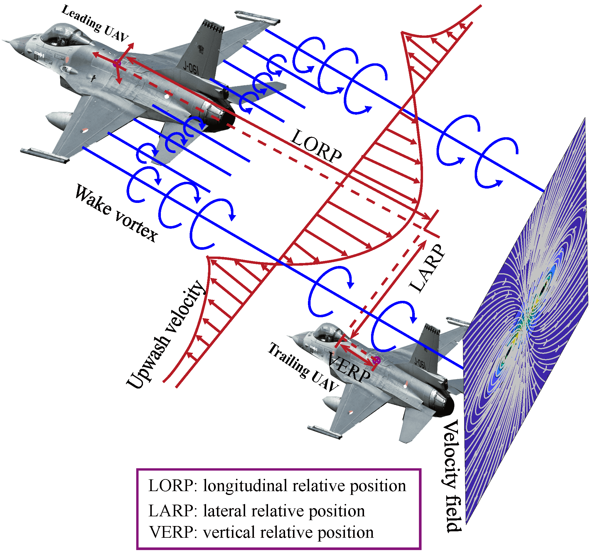
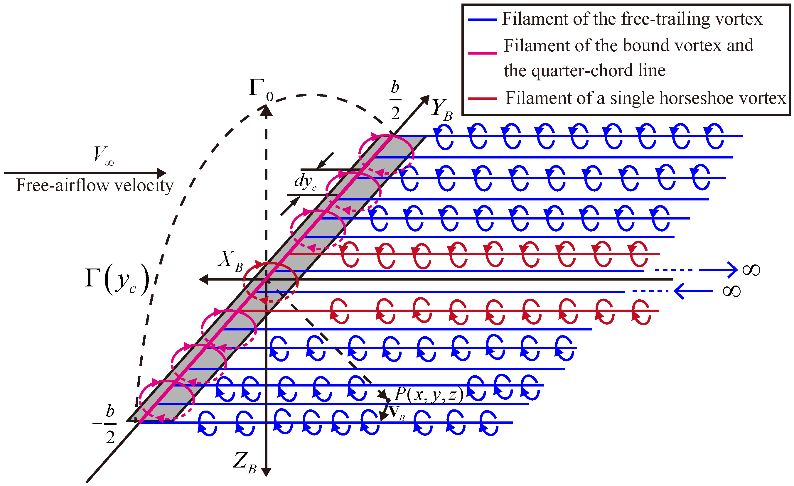
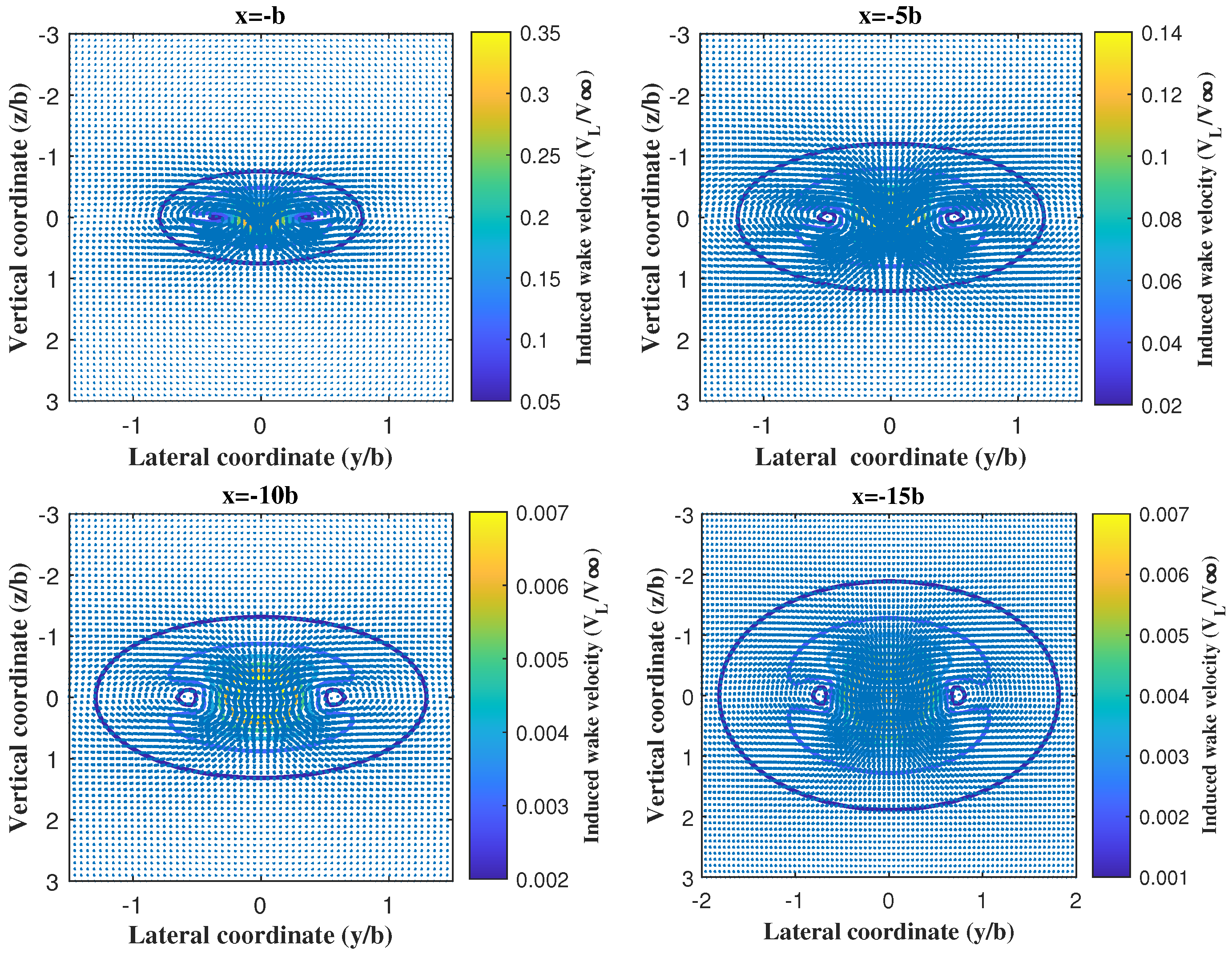
2.1. Wake Vortex Model

Taking into account the estimation accuracy and computational efficiency for real-time implementation, a continuous-horseshoe vortex method is employed to model the wake vortex. According to its modeling approach, the wake vortex comprises an infinite number of continuously distributed semi-infinite horseshoe vortices. Considering the structure of the horseshoe vortex, the wake vortex is divided into a bound vortex and a free-trailing vortex. The bound vortex adheres to the wing surface and the filaments follow along the quarter-chord line. The free-trailing vortex falls off the wing surface and the filaments extend downstream to infinity parallel to the velocity vector of the leading UAV.

In the case of an approximately rectangular wing, the lift of a UAV presents an elliptic distribution along the quarter-chord line. Therefore, the circulation distribution of the wake vortex is assumed to be

$$\Gamma \left(y_c\right)={\Gamma }_0\sqrt{1-{\left(\frac{2y_c}{b}\right)}^2},(-b/2\le y_c\le b/2)$$

(1)

where $y_c$ is the lateral coordinate of the point on the quarter-chord line and ${\Gamma }_0=2V_{\infty }S{C}_L/$$\left(b\pi \right)$ is the circulation at the wing root, with $V_{\infty }$ being the magnitude of the free-airflow velocity, S and b being the area and span of the wing, and $C_L$ denoting the lift coefficient. For an arbitrary point $P(x,y,z)$ inside the wake vortex, the velocity induced by a single straight vortex filament is obtained as follows according to the Kutta–Joukowski theorem and the Biot–Savart law,

$$\mathit{v}(x,y,z)=\frac{\Gamma \left(y_c\right)}{4\pi h}(cos{\theta }_0-cos{\theta }_{\infty })·\kappa ·\mathit{n}$$

(2)

where ${\theta }_0$ and ${\theta }_{\infty }$ are the initial and final angles formed by point P and the vortex filament, h is the perpendicular distance from point P to the vortex filament, $\kappa$ denotes the decrease in the strength of the wake vortex, and $\mathit{n}$ is the unit vector of the induced velocity.

Following the continuous-horseshoe vortex method, the magnitude of the wake velocity is calculated by integrating the induced velocity of the single straight vortex filament along the quarter-chord line. Therefore, the body frame $\mathcal{F}=\{O_B,X_B,Y_B,Z_B\}$ of the leading UAV is established to determine the location and orientation of the vortex filament. As illustrated in Figure 2, the origin $O_B$ is defined at the center of gravity (CG) of the leading UAV. $X_B$ points toward the nose of the leading UAV, $Y_B$ points toward the right wing, and $Z_B$ points toward the fuselage belly. It should be noted that the body frame is fixed to the leading UAV. On this basis and taking into account the geometric relationship between the angle and position in (2), the velocity components at point P in the body frame of the leading UAV are given by

$$\begin{array}{c}\hfill \left\{\begin{array}{cc}{V}_{f_{Y_B}}=\hfill & {\displaystyle {\int }_{-b/2}^{b/2}\kappa ·\mu ·\frac{\Gamma \left(y_c\right)z}{4\pi [{(y-y_c)}^2+z^2+r_c^2]}}\hfill \\ \hfill & ·\left(1-\frac{x}{\sqrt{x^2+{(y-y_c)}^2+z^2}}\right)·\mathrm{d}{y}_c\hfill \\ V_{f_{Z_B}}=\hfill & {\displaystyle {\int }_{-b/2}^{b/2}\kappa ·\mu ·\frac{\Gamma \left(y_c\right)(y-y_c)}{4\pi [{(y-y_c)}^2+z^2+r_c^2]}}\hfill \\ \hfill & ·\left(1-\frac{x}{\sqrt{x^2+{(y-y_c)}^2+z^2}}\right)·\mathrm{d}{y}_c\hfill \end{array}\right.\end{array}$$

(3)

$$\begin{array}{c}\hfill \left\{\begin{array}{cc}{V}_{b_{X_B}}=\hfill & {\displaystyle {\int }_{-b/2}^0\kappa ·\mu ·\frac{\Gamma \left(y_c\right)z}{4\pi (x^2+z^2)}}\hfill \\ \hfill & ·\left(\frac{y-y_c}{\sqrt{x^2+{(y-y_c)}^2+z^2}}-\frac{y+y_c}{\sqrt{x^2+{(y+y_c)}^2+z^2}}\right)·\mathrm{d}{y}_c\hfill \\ V_{b_{Z_B}}=\hfill & {\displaystyle {\int }_{-b/2}^0\kappa ·\mu ·\frac{\Gamma \left(y_c\right)x}{4\pi (x^2+z^2)}}\hfill \\ \hfill & ·\left(\frac{y-y_c}{\sqrt{x^2+{(y-y_c)}^2+z^2}}-\frac{y+y_c}{\sqrt{x^2+{(y+y_c)}^2+z^2}}\right)·\mathrm{d}{y}_c\hfill \end{array}\right.\end{array}$$

(4)

where $V_{f_{Y_B}}$ and $V_{f_{Z_B}}$ are induced by all filaments of the free-trailing vortex on the $Y_B$-axis and $Z_B$-axis, respectively; $V_{b_{X_B}}$ and $V_{b_{Z_B}}$ are induced by all filaments of the bound vortex on the $X_B$-axis and $Z_B$-axis, respectively; $r_c$ is the core radius of the free-trailing vortex introduced to eliminate the possible singular problem; and $\mu$ is the interaction coefficient of filaments. The wake velocity at point P is defined as ${\mathit{V}}_B=[V_{X_B},V_{Y_B},V_{Z_B}]$, where $V_{X_B}$, $V_{Y_B}$, and $V_{Z_B}$ are the velocity components on the $X_B$, $Y_B$, and $Z_B$ axes, respectively. Therefore, $V_{X_B}=V_{b_{X_B}}$,$V_{Y_B}=V_{f_{Y_B}}$, and $V_{Z_B}=V_{b_{Z_B}}+V_{f_{Z_B}}$. Note that $V_{X_B}$, $V_{Y_B}$, and $V_{Z_B}$ are also known as the backwash, sidewash, and upwash velocities, respectively.

The wake vortex effect refers to the forces and moments generated by the wake vortex of the leading UAV on the trailing UAV. Therefore, the wake vortex effect can be estimated according to the change in the attack angle for the trailing UAV. Let $\Delta \alpha$ represent the increment in the attack angle at an arbitrary point on the quarter-chord line of the trailing wing, which can be obtained using the wake velocity calculated above [14]. Note that the aerodynamic and geometric parameters used in the following equation to estimate the wake vortex effect are for the trailing UAV.

Based on a statistical strategy, the induced lift and drag are written as

$$\begin{array}{c}\hfill \left\{\begin{array}{c}\Delta L=q_{\infty }S{C}_{L_{\alpha }}\Delta \overline{\alpha }\hfill \\ \Delta D=q_{\infty }S\left({\left(C_L+C_{L_{\alpha }}\Delta \overline{\alpha }\right)}^2-C_L^2\right)/\left(\pi AR\right)\hfill \end{array}\right.\end{array}$$

(5)

where $\Delta \overline{\alpha }=\frac{1}{N}{\sum }_{i=1}^N\Delta {\alpha }_i$ is the average increment of the attack angle, with N being the number of statistical points; $q_{\infty }$ represents the dynamic pressure; $C_L$ is the lift coefficient; $C_{L_{\alpha }}$ is the lift curve slope; S is the wing area; and $AR$ is the aspect ratio of the wing that can be calculated by $AR=b^2/S$.

Unlike the induced forces, the arm of force at the statistical point must be taken into account for the calculation of the induced moments. Therefore, one has

$$\begin{array}{c}\hfill \left\{\begin{array}{c}\Delta \mathcal{L}=q_{\infty }S\left(\frac{1}{N}\sum _{i=1}^N{C}_{L_{\alpha }}\Delta {\alpha }_i\left(-y_{c_i}\right)\right)\hfill \\ \Delta \mathcal{M}=q_{\infty }S\left(\frac{1}{N}\sum _{i=1}^N{C}_{L_{\alpha }}\Delta {\alpha }_i\left(x_0-\left|y_{c_i}\right|tan\Lambda \right)\right)\hfill \end{array}\right.\end{array}$$

(6)

where $\Delta \mathcal{L}$ and $\Delta \mathcal{M}$ are the induced rolling and pitching moments, respectively; $y_{c_i}$ is the lateral arm of force at the i-th statistical point; $\Lambda$ is the sweep angle of the wing; and $x_0$ is the lateral coordinate of the aerodynamic center.

The wake vortex effect is introduced into the dynamic and kinematic equations of the trailing UAV in the form of the induced forces and moments. It should be noted that this statistical strategy can improve the calculation efficiency while ensuring estimation accuracy compared to the continuous calculation method.

Remark 1. 

The generated side force and yawing moment are mainly caused by the sidewash velocity acting on the vertical tail of the trailing UAV. However, both the sidewash velocity and the area of the vertical tail are very small. Therefore, the induced side force and yawing moment can be ignored.

2.2. Trailing UAV Model

The highly nonlinear wake vortex effect encountered by the trailing UAV eliminates the possibility of using a simple linear model to achieve an accurate characterization of UAV dynamics while flying in close formation. Therefore, the 6-DOF nonlinear high-fidelity aircraft model, which was utilized in [27], is employed. To incorporate the wake vortex effect, we modified the dynamic and kinematic equations of the trailing UAV,

$$\begin{array}{c}\hfill \left\{\begin{array}{cc}{\dot{x}}_E=\hfill & (u+\Delta u)\left(\cos \theta \cos \psi \right)\hfill \\ \hfill & +(v+\Delta v)(\sin \varphi \cos \psi \sin \theta -\cos \varphi \sin \psi )\hfill \\ \hfill & +(w+\Delta w)(\cos \varphi \sin \theta \cos \psi +\sin \varphi \sin \psi )\hfill \\ {\dot{y}}_E=\hfill & (u+\Delta u)\left(\sin \psi \cos \theta \right)\hfill \\ \hfill & +(v+\Delta v)(\sin \psi \sin \theta \sin \varphi +\cos \psi \cos \varphi )\hfill \\ \hfill & +(w+\Delta w)(\sin \psi \sin \theta \cos \varphi -\cos \psi \sin \varphi )\hfill \\ {\dot{z}}_E=\hfill & (u+\Delta u)\sin \theta -(v+\Delta v)\left(\cos \theta \sin \varphi \right)\hfill \\ \hfill & -(w+\Delta w)\left(\cos \theta \cos \varphi \right)\hfill \end{array}\right.\end{array}$$

(7)

$$\begin{array}{c}\hfill \left\{\begin{array}{cc}\dot{V}=\hfill & \frac{1}{m}(-(D+\Delta D)+F_T\cos \alpha \cos \beta )\hfill \\ \hfill & +g(-\cos \alpha \cos \beta \sin \theta +\sin \beta \sin \varphi \cos \theta \hfill \\ \hfill & +\sin \alpha \cos \beta \cos \varphi \cos \theta )\hfill \\ \dot{\alpha }=\hfill & q-(p\cos \alpha +r\sin \alpha )\tan \beta \hfill \\ \hfill & +\frac{1}{mV\cos \beta }(-(L+\Delta L)-F_T\sin \alpha )\hfill \\ \hfill & +\frac{1}{V\cos \beta }\left(g(\sin \alpha \sin \theta +\cos \alpha \cos \varphi \cos \theta )\right)\hfill \\ \dot{\beta }=\hfill & p\sin \alpha -r\cos \alpha +\frac{1}{mV}(Y-F_T\cos \alpha \sin \beta )\hfill \\ \hfill & +\frac{1}{V}\left(g\right(\cos \alpha \sin \beta \sin \theta +\cos \beta \sin \varphi \cos \theta \hfill \\ & -\sin \alpha \sin \beta \cos \varphi \cos \theta \left)\right)\hfill \end{array}\right.\end{array}$$

(8)

$$\begin{array}{c}\hfill \left\{\begin{array}{c}\dot{\varphi }=p+\tan \theta (q\sin \varphi +r\cos \varphi )\hfill \\ \dot{\theta }=q\cos \varphi -r\sin \varphi \hfill \\ \dot{\psi }=\sec \theta (q\sin \varphi +r\cos \varphi )\hfill \end{array}\right.\end{array}$$

(9)

$$\begin{array}{c}\hfill \left\{\begin{array}{c}\dot{p}=(c_{1}r+c_{2}p)q+c_3(\mathcal{L}+\Delta \mathcal{L})+c_4\mathcal{N}\hfill \\ \dot{q}=c_{5}pr-c_6(p^2-r^2)+c_7(\mathcal{M}+\Delta \mathcal{M})\hfill \\ \dot{r}=(c_{8}p-c_{2}r)q+c_4(\mathcal{L}+\Delta \mathcal{L})+c_9\mathcal{N}\hfill \end{array}\right.\end{array}$$

(10)

where $x_E$, $y_E$, and $z_E$ are the position coordinates in the inertial frame; V represents the velocity in the wind frame; $\alpha$ and $\beta$ are the aerodynamic angles; $\varphi$, $\theta$, and $\psi$ denote the attitude angles; p, q, and r are the angular rates; u, v, and w are the velocity components in the body frame, with $u=V\cos \alpha \cos \beta$, $v=V\sin \beta$, and $w=V\sin \alpha \cos \beta$; $\Delta u$, $\Delta v$, and $\Delta w$ refer to the components of the wake velocity in the body frame of the trailing UAV, which can be obtained by transforming ${\mathit{V}}_B$; L, D, Y and $\mathcal{L}$, $\mathcal{M}$, $\mathcal{N}$ represent the aerodynamic forces and moments, whose calculation processes are presented in [28]; $c_1$ to $c_9$ are the inertia coefficients, whose expressions are also demonstrated in [28]; m and g are the mass and gravity acceleration, respectively; and $\Delta L$, $\Delta D$ and $\Delta \mathcal{L}$, $\Delta \mathcal{M}$ are the induced forces and moments. The control inputs of the model are defined as the thrust $F_T$, the elevator ${\delta }_e$, the aileron ${\delta }_a$, and the rudder ${\delta }_r$.

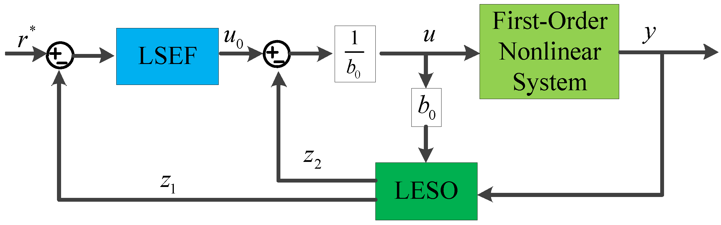
3. Structure of the First-Order LADRC

In this section, the first-order LADRC is investigated for the close-formation control system. The core idea of the LADRC is to estimate and compensate for various internal and external uncertainties of the control object by regarding them as a total disturbance. The LADRC is composed of two important parts, namely the linear extended-state observer (LESO) and the linear state-error feedback controller (LSEF).

Consider the following form of the first-order nonlinear system:

$$\begin{array}{c}\hfill \left\{\begin{array}{c}\dot{x}=f(x,t)+d\left(t\right)+bu\hfill \\ y=x\hfill \end{array}\right.\end{array}$$

(11)

where $f(x,t)$ is the internal uncertainty, $d\left(t\right)$ represents the external disturbance, x and y are the state and output of the system, u is the control input, and b is the gain. For the above nonlinear system, the overall control structure of the first-order LADRC is illustrated in Figure 3. Let $x_1=x,x_2=f(x,t)+d\left(t\right)+(b-b_0)u$, where $b_0$ is an estimate of the real b. Regard $x_2$ as the total disturbance of the system and call it the extended state. By assuming ${\dot{x}}_2=\xi$, the original nonlinear system can be transformed into an integral chain system that includes the total disturbance, as follows:

$$\begin{array}{c}\hfill \left\{\begin{array}{c}{\dot{x}}_1=x_2+b_{0}u\hfill \\ {\dot{x}}_2=\xi \hfill \\ y=x_1\hfill \end{array}\right.\end{array}$$

(12)

Then, the design process of the LESO and the LSEF are described for the transformed integral chain system.

LESO. The system state and total disturbance can be estimated using the LESO. A second-order extended-state observer is designed as

$$\begin{array}{c}\hfill \left\{\begin{array}{c}\epsilon =z_1-y\hfill \\ {\dot{z}}_1=z_2+l_1\epsilon +b_{0}u\hfill \\ {\dot{z}}_2=l_2\epsilon \hfill \end{array}\right.\end{array}$$

(13)

where $z_1$ and $z_2$ are the estimated values of the state $x_1$ and the total disturbance $x_2$, respectively, and $l_1$ and $l_2$ are the observer gains to be adjusted. It should be noted that the transformed integral chain system can be observed by the LESO if $l_1$ and $l_2$ are selected appropriately. The bandwidth method proposed by Gao is employed to determine the observer gains,

$$\begin{array}{c}\hfill \left\{\begin{array}{c}{l}_1=2\omega \hfill \\ l_2={\omega }^2\hfill \end{array}\right.\end{array}$$

(14)

where $\omega$ is the observer bandwidth.

LSEF. Based on the LESO, the total disturbance can be compensated for using the LSEF. The control signal after disturbance compensation is designed as

$$\begin{array}{c}\hfill u=\frac{u_0-z_2}{b_0}\end{array}$$

(15)

where $u_0$ is the control output of the LSEF. By ignoring the estimation error of $z_2\to x_2$ and substituting (15) into (12), one has

$$\begin{array}{c}\hfill \left\{\begin{array}{c}\dot{x}=u_0\hfill \\ y=x\hfill \end{array}\right.\end{array}$$

(16)

The transfer relationship from $u_0$ to y becomes integral. So far, the dynamic linearization for the original nonlinear system is realized by real-time disturbance estimation and compensation. For the integral system, the LSEF is designed as

$$\begin{array}{c}\hfill u_0=k_p(r^{*}-z_1)\end{array}$$

(17)

where $r^{*}$ is the reference signal and $k_p$ is the feedback gain.

Remark 2. 

The convergence of the LESO and the stability of the closed-loop LADRC have been proven under the assumption that the differentiation of the total disturbance is bounded. Furthermore, the estimation and compensation capacity for the total disturbance depends on the bandwidth of the LESO and the gain of the LSEF, respectively.

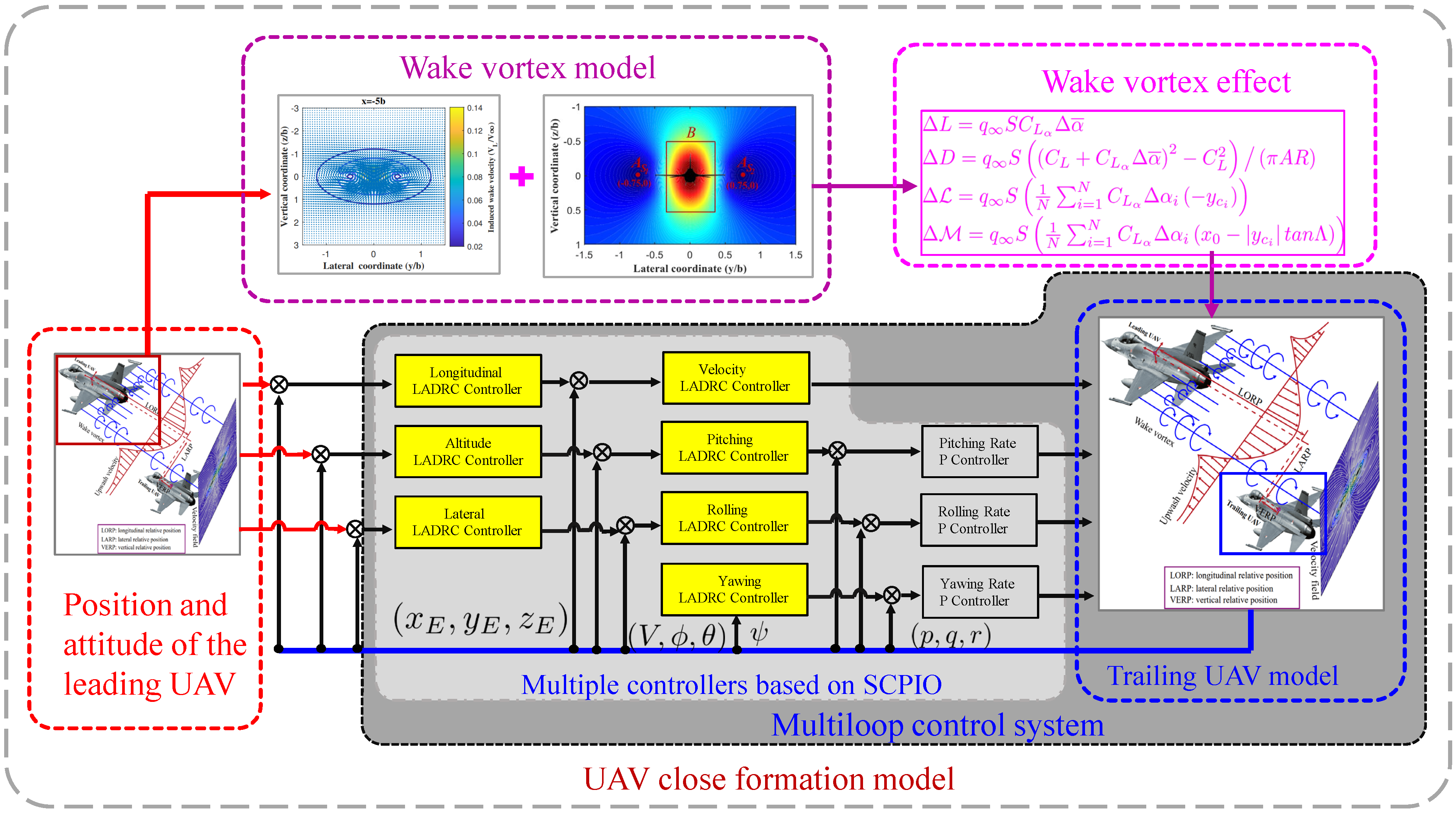
4. Robust Control System Design

From the modified model, the flight dynamics of the trailing UAV would be seriously disturbed by the wake vortex effect. Therefore, the robust close-formation control system is essential for enhancing flight stability and acquiring the maximum aerodynamic benefits.

4.1. Control Objective

The robust close-formation control system is implemented on the trailing UAV to steer it to the sweet spot and hold its position. The position of the sweet spot relative to the leading UAV is defined as $(\Delta x_{E_d},\Delta y_{E_d},\Delta z_{E_d})$ in the inertial frame. The tracking errors of the relative position components are calculated by

$$\begin{array}{c}\hfill \left\{\begin{array}{c}{e}_{x_E}=\Delta x_{E_d}-\Delta x_E\hfill \\ e_{y_E}=\Delta y_{E_d}-\Delta y_E\hfill \\ e_{z_E}=\Delta z_{E_d}-\Delta z_E\hfill \end{array}\right.\end{array}$$

(18)

where $\Delta x_E$, $\Delta y_E$, and $\Delta z_E$ are the actual relative position components of the trailing UAV. To acquire the maximum aerodynamic benefit, the control objectives for the three relative position components are specified as $\underset{t\to \infty }{lim}{e}_{x_E}=0$, $\underset{t\to \infty }{lim}{e}_{y_E}=0$, and $\underset{t\to \infty }{lim}{e}_{z_E}=0$. It should be noted that the control error of each relative position component is required to be less than $0.1b$ for an engineering application.

4.2. Control System Design

Given the dynamic characteristics of the trailing UAV, the control system is divided into three control subsystems for the longitudinal, altitude, and lateral channels. Considering the strength of the wake vortex effect, the control subsystem of each channel is composed of two cascade controllers, namely an outer-loop position LADRC controller and an inner-loop attitude LADRC controller. The overall scheme of the control system is shown in Figure 4. Although these channels are coupled with each other, the coupling effect can be incorporated into the total disturbance of the channel. Therefore, the control subsystems for these channels are designed independently using the first-order LADRC. It should be noted that the action mechanism of the control system is to receive the relative position components of the sweet spot and translate them into the control inputs for the trailing UAV.

Longitudinal Channel. According to the modified model, the longitudinal position $x_E$ is mainly related to the velocity V, which mainly depends on the thrust $F_T$. Therefore, the longitudinal channel can be divided into two cascade subsystems with strict-feedback form: the outer-loop longitudinal position subsystem and the inner-loop velocity subsystem. The outer-loop longitudinal position subsystem is defined by a first-order nonlinear system. The longitudinal position is considered the output and the velocity serves as the virtual input. The inner-loop velocity subsystem, on the other hand, is described by a first-order nonlinear system in which the velocity is the output variable and the input is provided by the thrust. Considering the principle of the first-order LADRC, the longitudinal channel is further transformed into a chain system including two first-order integral subsystems. They are

$$\begin{array}{c}\hfill \left\{\begin{array}{c}{\dot{x}}_E=f_{x_E}+b_{x_E}V\hfill \\ \dot{V}=f_V+b_V{F}_T\hfill \end{array}\right.\end{array}$$

(19)

where $f_{x_E}$ and $f_V$ are the total disturbance of the outer-loop longitudinal position subsystem and the inner-loop velocity subsystem, respectively, and $b_{x_E}=Vcos(\theta -\alpha )$ and $b_V=\frac{cos\alpha }{m}$ are the subsystem gains. The first-order LADRC controller is designed for each subsystem to dynamically estimate and compensate for the total disturbance, which can effectively suppress the transmission of the disturbance caused by the wake vortex effect. The specific forms are

$$\left\{\begin{array}{c}{\epsilon }_{x_E}=x_E-z_{1_{x_E}}\hfill \\ {\dot{z}}_{1_{x_E}}=z_{2_{x_E}}+l_{1_{x_E}}{\epsilon }_{x_E}\hfill \\ +b_{x_E}{V}^{*}\hfill \\ {\dot{z}}_{2_{x_E}}=l_{2_{x_E}}{\epsilon }_{x_E}\hfill \\ l_{1_{x_E}}=2{\omega }_{x_E}\hfill \\ l_{2_{x_E}}={\omega }_{x_E}^2\hfill \\ u_{0_{x_E}}=k_{p_{x_E}}(x_E^{*}-z_{1_{x_E}})\hfill \\ V^{*}=\left(u_{0_{x_E}}-z_{2_{x_E}}\right)/b_{x_E}\hfill \end{array}\right.\left\{\begin{array}{c}{\epsilon }_V=V-z_{1_V}\hfill \\ {\dot{z}}_{1_V}=z_{2_V}+l_{1_V}{\epsilon }_V\hfill \\ +b_V{F}_T\hfill \\ {\dot{z}}_{2_V}=l_{2_V}{\epsilon }_V\hfill \\ l_{1_V}=2{\omega }_V\hfill \\ l_{2_V}={\omega }_V^2\hfill \\ u_{0_V}=k_{p_V}(V^{*}-z_{1_V})\hfill \\ F_T=\left(u_{0_V}-z_{2_V}\right)/b_V\hfill \end{array}\right.$$

(20)

where $x_E^{*}$ is the reference signal of the outer-loop longitudinal position LADRC controller, $V^{*}$ is not only the output of the outer-loop longitudinal position LADRC controller but also the reference signal of the inner-loop velocity LADRC controller, $F_T$ is the output of the inner-loop velocity LADRC controller, and the meanings of the other parameters are consistent with those in Section 3.

Altitude Channel. Based on the modified model, the altitude $z_E$ is mainly determined by the pitching angle $\theta$, which is only controlled by the pitching angle rate q. Therefore, the altitude channel consists of two cascade subsystems with strict-feedback form: the outer-loop altitude subsystem and the inner-loop pitching-angle subsystem. Using the same transformation method as the longitudinal channel, the chain system of the altitude channel is

$$\begin{array}{c}\hfill \left\{\begin{array}{c}{\dot{z}}_E=f_{z_E}+b_{z_E}\theta \hfill \\ \dot{\theta }=f_{\theta }+b_{\theta }q\hfill \end{array}\right.\end{array}$$

(21)

where $f_{z_E}$ and $f_{\theta }$ are the total disturbance of the outer-loop altitude subsystem and the inner-loop pitching-angle subsystem, respectively, and $b_{z_E}=V(\pi /180)$ and $b_{\theta }=1$ are the subsystem gains. Similarly, the first-order LADRC controller of each subsystem is designed as

$$\left\{\begin{array}{c}{\epsilon }_{z_E}=z_E-z_{1_{z_E}}\hfill \\ {\dot{z}}_{1_{z_E}}=z_{2_{z_E}}+l_{1_{z_E}}{\epsilon }_{z_E}\hfill \\ +b_{z_E}{\theta }^{*}\hfill \\ {\dot{z}}_{2_{z_E}}=l_{2_{z_E}}{\epsilon }_{z_E}\hfill \\ l_{1_{z_E}}=2{\omega }_{z_E}\hfill \\ l_{2_{z_E}}={\omega }_{z_E}^2\hfill \\ u_{0_{z_E}}=k_{p_{z_E}}(z_E^{*}-z_{1_{z_E}})\hfill \\ {\theta }^{*}=\left(u_{0_{z_E}}-z_{2_{z_E}}\right)/b_{z_E}\hfill \end{array}\right.\left\{\begin{array}{c}{\epsilon }_{\theta }=\theta -z_{1_{\theta }}\hfill \\ {\dot{z}}_{1_{\theta }}=z_{2_{\theta }}+l_{1_{\theta }}{\epsilon }_{\theta }\hfill \\ +b_{\theta }{q}^{*}\hfill \\ {\dot{z}}_{2_{\theta }}=l_{2_{\theta }}{\epsilon }_{\theta }\hfill \\ l_{1_{\theta }}=2{\omega }_{\theta }\hfill \\ l_{2_{\theta }}={\omega }_{\theta }^2\hfill \\ u_{0_{\theta }}=k_{p_{\theta }}({\theta }^{*}-z_{1_{\theta }})\hfill \\ q^{*}=\left(u_{0_{\theta }}-z_{2_{\theta }}\right)/b_{\theta }\hfill \end{array}\right.$$

(22)

where $z_E^{*}$ is the reference signal of the outer-loop altitude LADRC controller, ${\theta }^{*}$ is not only the output of the outer-loop altitude LADRC controller but also the reference signal of the inner-loop pitching-angle LADRC controller, and $q^{*}$ is the output of the inner-loop pitching-angle LADRC controller.

Lateral Channel. Unlike the longitudinal and altitude channel, the lateral channel is further decomposed into two subchannels, namely the rolling subchannel and the yawing subchannel. Note that these two subchannels are closely coupled.

For the rolling subchannel, the lateral position $y_E$ is mainly related to the rolling angle $\varphi$, which is only affected by the rolling-angle rate p. Therefore, the rolling subchannel can be divided into two cascade subsystems with strict-feedback form: the outer-loop lateral-position subsystem and the inner-loop rolling-angle subsystem. Similarly, the chain system of the rolling subchannel is

$$\begin{array}{c}\hfill \left\{\begin{array}{c}{\dot{y}}_E=f_{y_E}+b_{y_E}\varphi \hfill \\ \dot{\varphi }=f_{\varphi }+b_{\varphi }p\hfill \end{array}\right.\end{array}$$

(23)

where $f_{y_E}$ and $f_{\varphi }$ are the total disturbance of the outer-loop lateral-position subsystem and the inner-loop rolling-angle subsystem, respectively, and $b_{y_E}=Vcos\alpha cos\beta cos\theta (\pi /180)$ and $b_{\varphi }=1$ are the subsystem gains. The first-order LADRC controller of each subsystem is formulated as

$$\left\{\begin{array}{c}{\epsilon }_{y_E}=y_E-z_{1_{y_E}}\hfill \\ {\dot{z}}_{1_{y_E}}=z_{2_{y_E}}+l_{1_{y_E}}{\epsilon }_{y_E}\hfill \\ +b_{y_E}{\varphi }^{*}\hfill \\ {\dot{z}}_{2_{y_E}}=l_{2_{y_E}}{\epsilon }_{y_E}\hfill \\ l_{1_{y_E}}=2{\omega }_{y_E}\hfill \\ l_{2_{y_E}}={\omega }_{y_E}^2\hfill \\ u_{0_{y_E}}=k_{p_{y_E}}(y_E^{*}-z_{1_{y_E}})\hfill \\ {\varphi }^{*}=\left(u_{0_{y_E}}-z_{2_{y_E}}\right)/b_{y_E}\hfill \end{array}\right.\left\{\begin{array}{c}{\epsilon }_{\varphi }=\varphi -z_{1_{\varphi }}\hfill \\ {\dot{z}}_{1_{\varphi }}=z_{2_{\varphi }}+l_{1_{\varphi }}{\epsilon }_{\varphi }\hfill \\ +b_{\varphi }{p}^{*}\hfill \\ {\dot{z}}_{2_{\varphi }}=l_{2_{\varphi }}{\epsilon }_{\varphi }\hfill \\ l_{1_{\varphi }}=2{\omega }_{\varphi }\hfill \\ l_{2_{\varphi }}={\omega }_{\varphi }^2\hfill \\ u_{0_{\varphi }}=k_{p_{\varphi }}({\varphi }^{*}-z_{1_{\varphi }})\hfill \\ p^{*}=\left(u_{0_{\varphi }}-z_{2_{\varphi }}\right)/b_{\varphi }\hfill \end{array}\right.$$

(24)

where $y_E^{*}$ is the reference signal of the outer-loop lateral-position LADRC controller, ${\varphi }^{*}$ is not only the output of the outer-loop lateral-position LADRC controller but also the reference signal of the inner-loop rolling-angle LADRC controller, and $p^{*}$ is the output of the inner-loop rolling-angle LADRC controller.

The yawing subchannel only includes the yawing-angle system. The chain system of the yawing subchannel is given as

$$\begin{array}{cc}\hfill & \dot{\psi }=f_{\psi }+b_{\psi }r\hfill \end{array}$$

(25)

where $\psi$ is the yawing angle, r is the yawing-angle rate, and $f_{\psi }$ is the total disturbance of the yawing-angle system. Due to the coupling effect of the rolling and yawing subchannels, the yawing is disturbed as rolling occurs. Therefore, the first-order LADRC controller is designed to compensate for this disturbance. The specific form is

$$\left\{\begin{array}{c}{\epsilon }_{\psi }=\psi -z_{1_{\psi }}\hfill \\ {\dot{z}}_{1_{\psi }}=z_{2_{\psi }}+l_{1_{\psi }}{\epsilon }_{\psi }+b_{\psi }{r}^{*}\hfill \\ {\dot{z}}_{2_{\psi }}=l_{2_{\psi }}{\epsilon }_{\psi }\hfill \\ l_{1_{\psi }}=2{\omega }_{\psi }\hfill \\ l_{2_{\psi }}={\omega }_{\psi }^2\hfill \\ u_{0_{\psi }}=-k_{p_{\psi }}{z}_{1_{\psi }}\hfill \\ r^{*}=\frac{u_{0_{\psi }}-z_{2_{\psi }}}{b_{\psi }}\hfill \end{array}\right.$$

(26)

where $r^{*}$ is the output of the yawing-angle LADRC controller.

Remark 3. 

According to the dynamic characteristics of the trailing UAV, the attitude rates of the altitude and lateral channels still need to be controlled. Therefore, a simple proportional (P) control is employed to add an attitude-rate control loop inside the attitude control loop. A trial-and-error tuning method is adopted to tune parameter P. The detailed design process of the attitude-rate control loop is omitted.

4.3. Stability Analysis of the Control System

To ensure the stability of the multiloop control system, this subsection mainly analyzes the stability of the entire error-feedback closed-loop control subsystem designed in Section 4.2. Before proceeding to the formal analysis, a theorem about the LESO of the LADRC is introduced.

Theorem 1. 

Assume that the total disturbance f of the system is differentiable and let $h=\dot{f}$. If h is bounded, there exists a constant ${\sigma }_i>0$ and a finite $T>0$ such that $|{\tilde{x}}_i\left(t\right)|\le {\sigma }_i,i=1,2,\cdots ,n+1,\forall t>T>0$ and $\omega >0$.

Proof. 

The proof of the theorem was previously established by Zhiqiang Gao [19] and is omitted here for brevity. □

According to Theorem 1, the observers designed in (20), (22), (24), and (26) are all stable. Building on this foundation, the stability analysis of the entire error-feedback closed-loop subsystem is described below. Construct a Lyapunov function of the following form for the multiloop control system of the UAV close-formation model:

$$V\left(\mathit{x}\right)=\frac{1}{2}{\mathit{e}}_1^T{\mathit{e}}_1+\frac{1}{2}{\mathit{e}}_2^T{\mathit{e}}_2+\frac{1}{2}{\mathit{e}}_3^T{\mathit{e}}_3$$

(27)

where $\mathit{x}$ represents the state variables of the multiloop control system and ${\mathit{e}}_1$, ${\mathit{e}}_2$, and ${\mathit{e}}_3$ are the tracking errors of the position loop, attitude loop, and angular-rate loop, respectively. Therefore, the entire multiloop control system is asymptotically stable as long as $\dot{V}\left(\mathit{x}\right)<0$. Next, this is proven by adding each loop incrementally from the inner loop to the outer loop.

Angular-Rate Loop Stability Analysis. The tracking error of the angular-rate loop is ${\mathit{e}}_3={\mathit{x}}_3^c-{\mathit{x}}_3$, where ${\mathit{x}}_3^c={[P^c,Q^c,R^c]}^T$ is the command signal. For this error, the Lyapunov function $V_3\left({\mathit{x}}_3\right)$ is constructed as follows:

$$V\left({\mathit{x}}_3\right)=\frac{1}{2}{\mathit{e}}_3^T{\mathit{e}}_3$$

(28)

To accelerate the response speed, the attitude angular-rate loop adopts the P control. By tuning the appropriate values ${\mathit{k}}_3=[k_p,k_Q,k_R]$ for the P parameters of each control channel, it can be guaranteed that $\dot{V}\left({\mathit{x}}_3\right)<0$. This implies that the tracking error ${\mathit{e}}_3$ converges asymptotically to zero and ${\mathit{x}}_3$ converges asymptotically to ${\mathit{x}}_3^c$.

Attitude Loop Stability Analysis. The tracking error of the attitude loop is defined as ${\mathit{e}}_2={\mathit{x}}_2^c-{\widehat{\mathit{x}}}_2$, where ${\mathit{x}}_2=[V,\varphi ,\theta ,\psi ]$ is the state variable of the attitude loop and ${\widehat{\mathit{x}}}_2$ denotes the estimated values of the state variables from the designed LESO. For the attitude loop, construct the following Lyapunov function

$$\begin{array}{c}\hfill V({\mathit{x}}_2,{\mathit{x}}_3)=\frac{1}{2}{\mathit{e}}_2^T{\mathit{e}}_2+\frac{1}{2}{\mathit{e}}_3^T{\mathit{e}}_3=\frac{1}{2}{\mathit{e}}_2^T{\mathit{e}}_2+V\left({\mathit{x}}_3\right)\end{array}$$

(29)

It should be pointed out that because the attitude loop includes the angular-rate loop, its tracking error must be taken into account when designing the Lyapunov function for the attitude loop. Assuming that the observation errors of the states and total disturbances are ${\sigma }_{2_1}$ and ${\sigma }_{2_2}$, then ${\widehat{\mathit{x}}}_2={\mathit{x}}_2+{\sigma }_{2_1}$ and ${\widehat{\mathit{f}}}_2={\mathit{f}}_2+{\sigma }_{2_2}$. For the error ${\mathit{e}}_3$, the state ${\mathit{x}}_3$ of the angular-rate loop converges asymptotically to the command signal ${\mathit{x}}_3^c$. Assuming that the convergence error is ${\epsilon }_3$, then ${\mathit{u}}_2={\mathit{x}}_3^c={\mathit{x}}_3+{\epsilon }_3$, i.e., ${\mathit{x}}_3={\mathit{u}}_2-{\epsilon }_3$. Combining the control variable ${\mathit{u}}_2$ of the attitude loop in (20), (22), (24), and (26), the derivative of the Lyapunov function is calculated by

$$\begin{array}{cc}\hfill \dot{V}({\mathit{x}}_2,{\mathit{x}}_3)=& {\mathit{e}}_2^T{\dot{\mathit{e}}}_2+\dot{V}\left({\mathit{x}}_3\right)\hfill \\ \hfill =& {\mathit{e}}_2^T({\dot{\mathit{x}}}_2^c-{\dot{\mathit{x}}}_2-{\dot{\sigma }}_{2_1})+\dot{V}\left({\mathit{x}}_3\right)\hfill \\ \hfill =& {\mathit{e}}_2^T({\dot{\mathit{x}}}_2^c-{\mathit{f}}_2-{\mathit{b}}_2{\mathit{x}}_2-{\dot{\sigma }}_{2_1})+\dot{V}\left({\mathit{x}}_3\right)\hfill \\ \hfill =& {\mathit{e}}_2^T({\dot{\mathit{x}}}_2^c-{\mathit{f}}_2-{\mathit{b}}_2({\mathit{u}}_2-{\epsilon }_3)-{\dot{\sigma }}_{2_1})+\dot{V}\left({\mathit{x}}_3\right)\hfill \\ \hfill =& {\mathit{e}}_2^T({\dot{\mathit{x}}}_2^c-{\mathit{b}}_2{\mathit{b}}_2^{-1}({\mathit{k}}_2{\mathit{e}}_2+{\dot{\mathit{x}}}_2^c-{\mathit{f}}_2-{\sigma }_{2_2})+{\mathit{b}}_2{\epsilon }_3-{\dot{\sigma }}_{2_1})+\dot{V}\left({\mathit{x}}_3\right)\hfill \\ \hfill =& {\mathit{e}}_2^T(-{\mathit{k}}_2{\mathit{e}}_2+{\mathit{b}}_2{\epsilon }_3+{\sigma }_{2_2}-{\dot{\sigma }}_{2_1})+\dot{V}\left({\mathit{x}}_3\right)\hfill \\ \hfill \le & -\parallel {\mathit{e}}_2^T\parallel ({\mathit{k}}_2\parallel {\mathit{e}}_2\parallel -\parallel {\mathit{b}}_2{\epsilon }_3+{\sigma }_{2_2}-{\dot{\sigma }}_{2_1}\parallel )+\dot{V}\left({\mathit{x}}_3\right)\hfill \end{array}$$

(30)

where ${\mathit{b}}_2$ is the control-gain vector of the attitude loop and ${\mathit{k}}_2$ is the error-proportional coefficient vector of the attitude angles. It should be noted that due to the existence of $\dot{V}\left({\mathit{x}}_3\right)$, the error-proportional coefficient of the attitude loop also includes ${\mathit{k}}_3$. Due to the convergence of the LESO and the angular-rate loop, ${\epsilon }_3,{\sigma }_{2_2}$, and ${\dot{\sigma }}_{2_1}$ are all bounded. Therefore, by tuning the appropriate values for ${\mathit{k}}_2$ and ${\mathit{k}}_3$, it can be ensured that $\dot{V}({\mathit{x}}_2,{\mathit{x}}_3)<0$. This implies that the tracking error ${\mathit{e}}_2$ asymptotically converges to zero and ${\widehat{\mathit{x}}}_2$ asymptotically converges to ${\mathit{x}}_2^c$. Furthermore, as ${\widehat{\mathit{x}}}_2$ asymptotically converges to ${\mathit{x}}_2$, the attitude-angle state ${\mathit{x}}_2$ asymptotically converges to ${\mathit{x}}_2^c$. It is worth noting that the velocity loop of the attitude loop does not include the angular-rate loop but rather takes the thrust of the trailing UAV as input. However, the error analysis process for the velocity loop is similar to that of other attitude-angle variables. Therefore, there is no separate analysis for the velocity loop.

Position Loop Stability Analysis. Similarly, the tracking error of the position loop is ${\mathit{e}}_1={\mathit{x}}_1^c-{\widehat{\mathit{x}}}_1$, where ${\mathit{x}}_1=[x_E,y_E,z_E]$. For this error, the Lyapunov function for the position loop is constructed using the same structure as previously mentioned

$$V({\mathit{x}}_1,{\mathit{x}}_2,{\mathit{x}}_3)=\frac{1}{2}{\mathit{e}}_1^T{\mathit{e}}_1+\frac{1}{2}{\mathit{e}}_2^T{\mathit{e}}_2+\frac{1}{2}{\mathit{e}}_3^T{\mathit{e}}_3=\frac{1}{2}{\mathit{e}}_1^T{\mathit{e}}_1+V({\mathit{x}}_2,{\mathit{x}}_3)$$

(31)

It is essential to point out that the Lyapunov function of the position loop is exactly the Lyapunov function of the multiloop control system (27). Assuming that the observation errors of the states and the total disturbances are ${\mathit{\sigma }}_{1_1}$ and ${\mathit{\sigma }}_{1_2}$, then ${\widehat{\mathit{x}}}_1={\mathit{x}}_1+{\mathit{\sigma }}_{1_1}$ and ${\widehat{\mathit{f}}}_1={\mathit{f}}_1+{\mathit{\sigma }}_{1_2}$. For the error ${\mathit{e}}_2$, the state ${\mathit{x}}_2$ of the angular-rate loop converges asymptotically to the command signal ${\mathit{x}}_2^c$. Assuming that the convergence error is ${\mathit{\epsilon }}_2$, then ${\mathit{u}}_1={\mathit{x}}_2^c={\mathit{x}}_2+{\mathit{\epsilon }}_2$, i.e., ${\mathit{x}}_2={\mathit{u}}_1-{\mathit{\epsilon }}_2$. Similar to the analysis process for the attitude loop, the derivative of the Lyapunov function is given by

$$\begin{array}{cc}\hfill \dot{V}({\mathit{x}}_1,{\mathit{x}}_2,{\mathit{x}}_3)=& {\mathit{e}}_1^T(-{\mathit{k}}_1{\mathit{e}}_1+{\mathit{b}}_1{\mathit{\epsilon }}_2+{\mathit{\sigma }}_{1_2}-{\dot{\mathit{\sigma }}}_{1_1})+\dot{V}({\mathit{x}}_2,{\mathit{x}}_3)\hfill \\ \hfill \le & -\parallel {\mathit{e}}_1^T\parallel ({\mathit{k}}_1\parallel {\mathit{e}}_1\parallel -\parallel {\mathit{b}}_1{\mathit{\epsilon }}_2+{\mathit{\sigma }}_{1_2}-{\dot{\mathit{\sigma }}}_{1_1}\parallel )+\dot{V}({\mathit{x}}_2,{\mathit{x}}_3)\hfill \end{array}$$

(32)

Therefore, one can draw a similar conclusion that by tuning the appropriate values for ${\mathit{k}}_1$, ${\mathit{k}}_2$, and ${\mathit{k}}_3$, it can be ensured that $\dot{V}({\mathit{x}}_1,{\mathit{x}}_2,{\mathit{x}}_3)<0$, which means that the derivative of the Lyapunov function of the multiloop control system for the UAV close-formation model is $\dot{V}\left(\mathit{x}\right)<0$.

In summary, the entire multiloop control system for the UAV close-formation model is asymptotically stable.

5. Sine-Powered Pigeon-Inspired Optimization

In the designed control system, each first-order LADRC controller has two control parameters, namely the feedback gain $k_{p_{*}}$ and the observer bandwidth ${\omega }_{*}$ ($*=x_E,V,z_E,\theta ,y_E,\varphi ,\psi$). Therefore, the control subsystem of the longitudinal and altitude channels contains four control parameters and the control subsystem of the lateral channel includes six control parameters. Due to the cascade structure of the control subsystem, the correlation among the control parameters is very high. To consider all control parameters together and find their optimal values, the tuning of the control parameters is restructured as an optimization problem. Sine-powered controlled PIO is utilized to optimize the control parameters of the control subsystem of each channel.

5.1. Standard PIO Algorithm

The standard PIO algorithm is divided into the map and compass operator and the landmark operator to perform a search based on the homing behavior of pigeons. Using the two operators can achieve better performance in searching for the global optimal position. It is assumed that there are $N^{pig}$ pigeons in the $D^{pig}$-dimension search space. The position and velocity of the i-th pigeon are ${\mathit{X}}_i^{pig}=[x_{i_1}^{pig},x_{i_2}^{pig},\cdots ,x_{i_{D^{pig}}}^{pig}]$ and ${\mathit{V}}_i^{pig}=[v_{i_1}^{pig},v_{i_2}^{pig},\cdots ,v_{i_{D^{pig}}}^{pig}]$, respectively. They are updated in each iteration.

Map and Compass Operator. In the map and compass operator, the new position and velocity of the i-th pigeon at the $N_C$-th iteration are calculated by

$$\begin{array}{c}\hfill \left\{\begin{array}{c}{\mathit{V}}_i^{pig}\left(N_C\right)={\mathit{V}}_i^{pig}(N_C-1)e^{-R{N}_C}\hfill \\ +rand·\left({\mathit{X}}_{gbest}^{pig}-{\mathit{X}}_i^{pig}(N_C-1)\right)\hfill \\ {\mathit{X}}_i^{pig}\left(N_C\right)={\mathit{X}}_i^{pig}(N_C-1)+{\mathit{V}}_i^{pig}\left(N_C\right)\hfill \end{array}\right.\end{array}$$

(33)

where R is the map and compass factor; $rand$ represents a random number with $rand\in [0,1]$; and ${\mathit{X}}_{gbest}^{pig}$ is the current global optimal position, which can be obtained by comparing the fitness value with all the positions of the pigeons. When the number of iterations reaches $N_{C_{1max}}^{pig}$, stop the current operator and proceed to the landmark operator.

Landmark Operator. In the landmark operator, the pigeon with the lowest fitness value will be abandoned. This decreases the number of pigeons by half in each iteration and the remaining pigeons update their positions according to the center of the pigeons, which can be described as

$$\begin{array}{c}\hfill \left\{\begin{array}{c}{N}^{pig}\left(N_C\right)=\frac{N^{pig}(N_C-1)}{2}\hfill \\ {\mathit{X}}_c^{pig}\left(N_C\right)=\frac{{\sum }_{i=1}^{N^{pig}\left(N_C\right)}{\mathit{X}}_i^{pig}(N_C-1)Fit\left({\mathit{X}}_i^{pig}(N_C-1)\right)}{{\sum }_{i=1}^{N^{pig}\left(N_C\right)}Fit\left({\mathit{X}}_i^{pig}(N_C-1)\right)}\hfill \\ {\mathit{X}}_i^{pig}\left(N_C\right)={\mathit{X}}_i^{pig}(N_C-1)\hfill \\ +rand·({\mathit{X}}_c^{pig}\left(N_C\right)-{\mathit{X}}_i^{pig}(N_C-1))\hfill \end{array}\right.\end{array}$$

(34)

where ${\mathit{X}}_c^{pig}$ denotes the center position of all the pigeons. Note that $Fit\left({\mathit{X}}_i^{pig}(N_C-1)\right)=1/fit\left({\mathit{X}}_i^{pig}(N_C-1)\right)$, where $fit(·)$ is the fitness function. The whole algorithm ends after another $N_{C_{2max}}^{pig}$ iterations.

5.2. SCPIO Algorithm

In the map and compass operator of the standard PIO, the map and compass factor R can balance the global exploration and local exploitation of the whole pigeon group. Global exploration is strengthened if R is relatively large; conversely, local exploitation can be enhanced. However, a fixed R is always adopted in the map and compass operator of the standard PIO. As a result, R has not made a contribution to the balance of global exploration and local exploitation. Therefore, a sine-powered controlled improvement strategy is employed to adjust R dynamically with the iterations. The adjustment formula is written as

$$\begin{array}{c}\hfill \left\{\begin{array}{c}R\left(N_C\right)=r\left(N_C\right)·\sin \left(\pi R(N_C-1)\right)\hfill \\ r\left(N_C\right)=r_{max}-N_C·(r_{max}-r_{min})/N_{C_{max}}\hfill \end{array}\right.\end{array}$$

(35)

where r is the control parameter in the range of $(0,1)$; $r_{max}$ and $r_{min}$ are the specified maximum and minimum values, respectively; and $N_{C_{max}}^{pig}$ represents the maximum number of iterations. The random nature of R is gradually weakened with the iterations. This indicates that the dynamic adjustment strategy of R retains the advantages of traversing and randomizing the weight in the early iterations, which urges the pigeons to perform extensive global exploration. In the later iterations, the pigeons gather around the global optimal position and the low flight velocity enables the pigeons to perform a fine search. Furthermore, the new position of each pigeon is obtained by simply adding the previous position ${\mathit{X}}_i^{pig}(N_C-1)$ and the current velocity ${\mathit{V}}_i^{pig}\left(N_C\right)$ in the map and compass operator of the standard PIO. Although the global exploration and local exploitation of the algorithm have been balanced by adjusting R dynamically, this balance may be conservative since the relationship between the position and velocity is not considered. According to [26], the position-update formula with the dynamic weight is given as follows

$$\begin{array}{cc}\hfill {\mathit{X}}_i^{pig}\left(N_C\right)=& {\omega }_i^{pig}\left(N_C\right)·{\mathit{X}}_i^{pig}(N_C-1)\hfill \\ \hfill & +{\omega }_i^{pi{g}^{{}^{\prime }}}\left(N_C\right)·{\mathit{V}}_i^{pig}\left(N_C\right)\hfill \\ \hfill & +rand·\sigma \left(N_C\right)·{\mathit{X}}_{gbest}^{pig}\hfill \end{array}$$

(36)

where ${\omega }_i^{pig}$ and ${\omega }_i^{pi{g}^{{}^{\prime }}}$ are the dynamic weights of the position and velocity of the i-th pigeon, respectively, and $\sigma$ is the acceleration coefficient. They are calculated by

$$\begin{array}{c}\hfill \left\{\begin{array}{c}{\omega }_i^{pig}\left(N_C\right)=\sigma \left(N_C\right)=\frac{exp\left(\frac{fit\left({\mathit{X}}_i^{pig}\left(N_C\right)\right)}{\overline{fit\left(N_C\right)}}\right)}{{\left(1+exp\left(-\frac{fit\left({\mathit{X}}_i^{pig}\left(N_C\right)\right)}{\overline{fit\left(N_C\right)}}\right)\right)}^{N_C}}\hfill \\ {\omega }_i^{pi{g}^{{}^{\prime }}}\left(N_C\right)=1-{\omega }_i^{pig}\left(N_C\right)\hfill \end{array}\right.\end{array}$$

(37)

where $\overline{fit\left(N_C\right)}$ is the average fitness value of all pigeons at the $N_C$-th iteration.

Note that the standard PIO that has been improved by using the sine-powered controlled strategy is abbreviated as SCPIO.

Remark 4. 

In the landmark operator of the standard PIO, all pigeons will move toward the center position, which implies that the movement direction of each pigeon is definite. Therefore, there is little room for improvement according to the action mechanism of the landmark operator. Considering this fact, SCPIO still adopts the landmark operator of the standard PIO.

5.3. Construction of the Fitness Function

According to the control objective, the integrated-time absolute error (ITAE) criterion is employed to construct the performance index, namely the fitness function, for the optimal design of the control system. On the one hand, the ITAE criterion includes two factors: time and error, which can take into account both the dynamic performance and stable performance of the control system and simultaneously ensure the response speed and stable accuracy. On the other hand, the ITAE criterion emphasizes the effect of the recent response, which can minimize the influence of the large initial error on the dynamic process. Furthermore, the attitude ITAE criterion of the trailing UAV is also incorporated into the fitness function to reduce the attitude oscillation in the position responses. Since the control system is composed of three control subsystems for different channels, the parameter optimization of the control system is transformed into the parameter optimization of three control subsystems.

Therefore, the fitness functions of three control subsystems for different channels are given as follows

$$\begin{array}{c}\hfill \left\{\begin{array}{c}{\displaystyle J_{Lon}=k_{e_{x_E}}{\int }_0^{t_T}t|e_{x_E}|\mathrm{d}t+k_{\Delta V}{\int }_0^{t_T}t|\Delta V|\mathrm{d}t}\hfill \\ {\displaystyle J_{Alt}=k_{e_{z_E}}{\int }_0^{t_T}t|e_{z_E}|\mathrm{d}t+k_{\Delta \theta }{\int }_0^{t_T}t|\Delta \theta |\mathrm{d}t}\hfill \\ {\displaystyle J_{Lat}=k_{e_{y_E}}{\int }_0^{t_T}t|e_{y_E}|\mathrm{d}t+k_{\Delta \varphi }{\int }_0^{t_T}t|\Delta \varphi |\mathrm{d}t}\hfill \\ {\displaystyle +k_{\Delta \psi }{\int }_0^{t_T}t|\Delta \psi |\mathrm{d}t}\hfill \end{array}\right.\end{array}$$

(38)

where $fi{t}_{Lon}$, $fi{t}_{Alt}$, and $fi{t}_{Lat}$ are the fitness functions of the longitudinal, altitude, and lateral channel, respectively; $e_{x_E}$, $e_{z_E}$, and $e_{y_E}$ are the tracking errors between the sweet spot and the actual relative position; $\Delta V$, $\Delta \theta$, $\Delta \varphi$, and $\Delta \psi$ are the velocity and attitude disturbances; $k_{*}(\ast =e_{x_E},e_{z_E},e_{y_E},\Delta V,\Delta \theta ,\Delta \varphi ,\Delta \psi )$ represents the weight coefficient; and $t_T$ denotes the simulation termination time of the control system. By minimizing the fitness function, the optimal control parameters of the control subsystem can be obtained.

5.4. Optimization Procedure

Since the control subsystem is designed independently according to the channel, the parameter optimization of the control subsystem for the longitudinal channel is taken as an example. Using the SCPIO algorithm, the detailed optimization procedures for the optimal control parameters are described as follows:

Step 1. 

Initialize the SCPIO parameters, including the number of pigeons $N^{pig}$, the dimension of thesearch space $D^{pig}$, the maximum and minimum values of the map and compass factor $r_{max}$ and $r_{min}$, the iteration numbers of two operators $N_{C_{1max}}^{pig}$ and $N_{C_{2max}}^{pig}$, and the position ${\mathit{X}}_i^{pig}$ and velocity ${\mathit{V}}_i^{pig}$ of all pigeons.

Step 2. 

Drive the close-formation simulation system using the pigeons in Step 1 to calculate the fitness function. Compare the fitness value and find the current optimal position.

Step 3. 

Conduct the iteration. If $N_C\le N_{C_{1max}}^{pig}$, perform the improved map and compass operator to update the pigeons. Then, drive the close-formation simulation system using the updated pigeons to calculate the fitness function. Update the optimal position by comparing the new fitness values with the current optimal one. When $N_{C_{1max}}^{pig}<N_C$, perform the landmark operator to continue the similar optimization process.

Step 4. 

Once the iteration time reaches $N_{C_{1max}}^{pig}+N_{C_{2max}}^{pig}$, terminate the algorithm and output the optimal position ${\mathit{X}}_{gbest}^{pig}$.

The pseudocode of the above steps is given in Algorithm 1.

Algorithm 1: SCPIO.

6. Simulation Results and Analysis

In this section, the simulation verification is conducted for a leading-trailing UAV close formation based on the F-16 aircraft model that serves two main purposes. The first is to determine the location of the sweet spot for the trailing UAV in close-formation flight. This is achieved by analyzing the variations in the wake vortex effect with the relative position to the leading UAV based on the established wake vortex model. The second is to validate the tracking performance of the designed robust close-formation control system via the SCPIO under the wake vortex effect. Furthermore, the robust close-formation control system based on a PI structure is used for comparison to more intuitively display the advantages of the designed control system. Both the inner and outer loops of the longitudinal and lateral channels adopt the P controller. The PI controller is developed for the outer loop of the altitude channel and the inner loop still adopts the P controller. Similarly, the parameter of each controller for the three channels also needs to be tuned.

In the simulation results, it is assumed that the leading UAV maintains a level and stable flight path at a speed of 152 m/s and an altitude of 4605 m, with attack and pitch angles of 4.5 deg. The initial flight states of the trailing UAV are $x_E\left(0\right)=0$ m, $y_E\left(0\right)=0$ m, $z_E\left(0\right)=4572$ m, $V\left(0\right)=152$ m/s, $\alpha \left(0\right)=4.5$ deg, $\beta \left(0\right)=0$ deg, $\varphi \left(0\right)=0$ deg, $\theta \left(0\right)=4.5$ deg, $\psi \left(0\right)=0$ deg, $p\left(0\right)=0$ deg/s, $q\left(0\right)=0$ deg/s, and $r\left(0\right)=0$ deg/s. The initial relative position between the leading and trailing UAV is set to $\Delta \mathit{P}(\Delta x_E,\Delta y_E,\Delta z_E)=[-14b,-2.9b,-3.6b]$. The modeling parameters of the wake vortex are specified as $V_{\infty }=152$ m/s, $\mu =1.6$, $C_L=0.2134$, and $C_{L_{\alpha }}=0.0422$, $N=100$. The aerodynamic derivatives, mass properties, and structural parameters of the F-16 aircraft model are given in [27]. The robust close-formation control system is applied to the trailing UAV to steer it to the sweet spot.

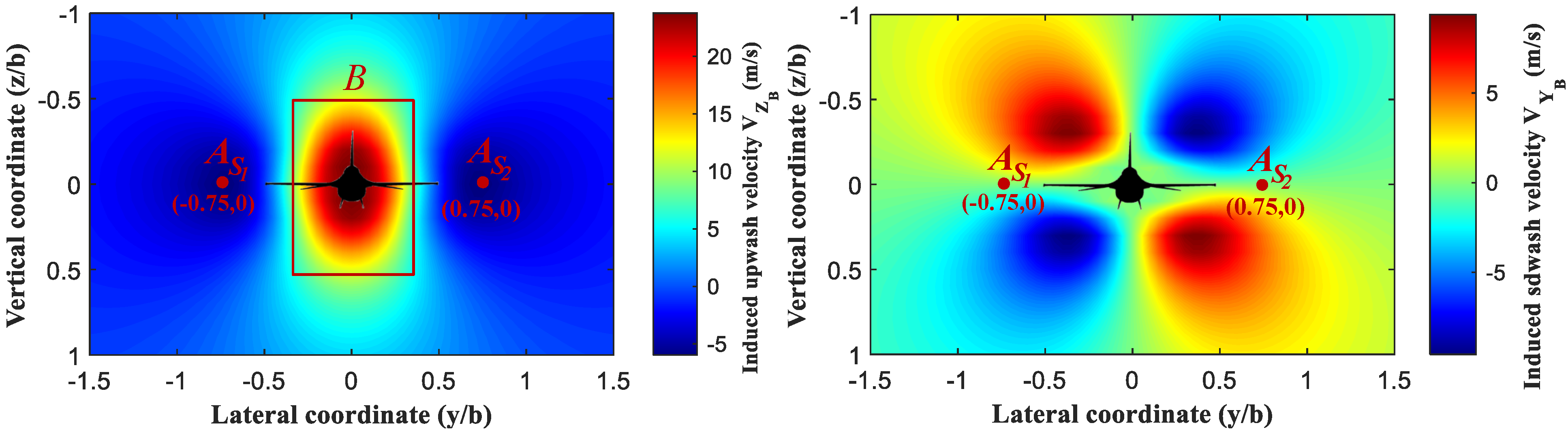
6.1. Analysis of the Sweet Spot

According to the continuous-horseshoe vortex method, the intensity of the wake vortex can be described as a function of the position in the body frame of the leading UAV. The variation of the dimensionless velocity field induced by the wake vortex with the longitudinal position is illustrated in Figure 5. We can see that the intensity of the induced velocity field decreases significantly with the negative increase in the longitudinal position. Furthermore, the intensity decays almost to zero when $x<-10b$, which implies that the wake vortex effect disappears completely. Therefore, the downstream longitudinal position should not exceed $10b$ if one wants to utilize the wake vortex effect of the leading UAV. The position of the sweet spot relative to the leading UAV is denoted as $(\Delta x_{B_d},\Delta y_{B_d},\Delta z_{B_d})$ in the body frame of the leading UAV. Considering the fuselage length of the UAV and the minimum safe spacing of close formation, the longitudinal relative position component $\Delta x_{B_d}$ of the sweet spot is set at $-3b$ to maximize the wake vortex effect. The variation of the induced velocity with the lateral and vertical positions calculated at $x=-3b$ is demonstrated in Figure 6. Two sweet spots $A_{s_1}$ and $A_{s_2}$ can be seen and their positions are consistent with earlier findings [6]. At the sweet spot, the maximum induced upwash velocity occurs and the induced sidewash velocity is relatively small. Therefore, the lateral and vertical relative position components are $\Delta y_{B_d}=\pm 0.75b$ and $\Delta z_{B_d}=0$, respectively. The trailing UAV should be driven toward the sweet spot and maintained in that position during close-formation flight. Note that the region designated by B is the area with the maximum downwash velocity, where the trailing UAV should be forbidden to appear. This means that the robust close-formation control system needs to have high control accuracy for the trailing UAV. Note that the position of the sweet spot is analyzed by the separation distance relative to the leading UAV, which makes the position independent of the coordinate frame. Therefore, the relative position $(\Delta x_{E_d},\Delta y_{E_d},\Delta z_{E_d})$ of the sweet spot in the inertial frame is still $(-3b,\pm 0.75b,0)$.

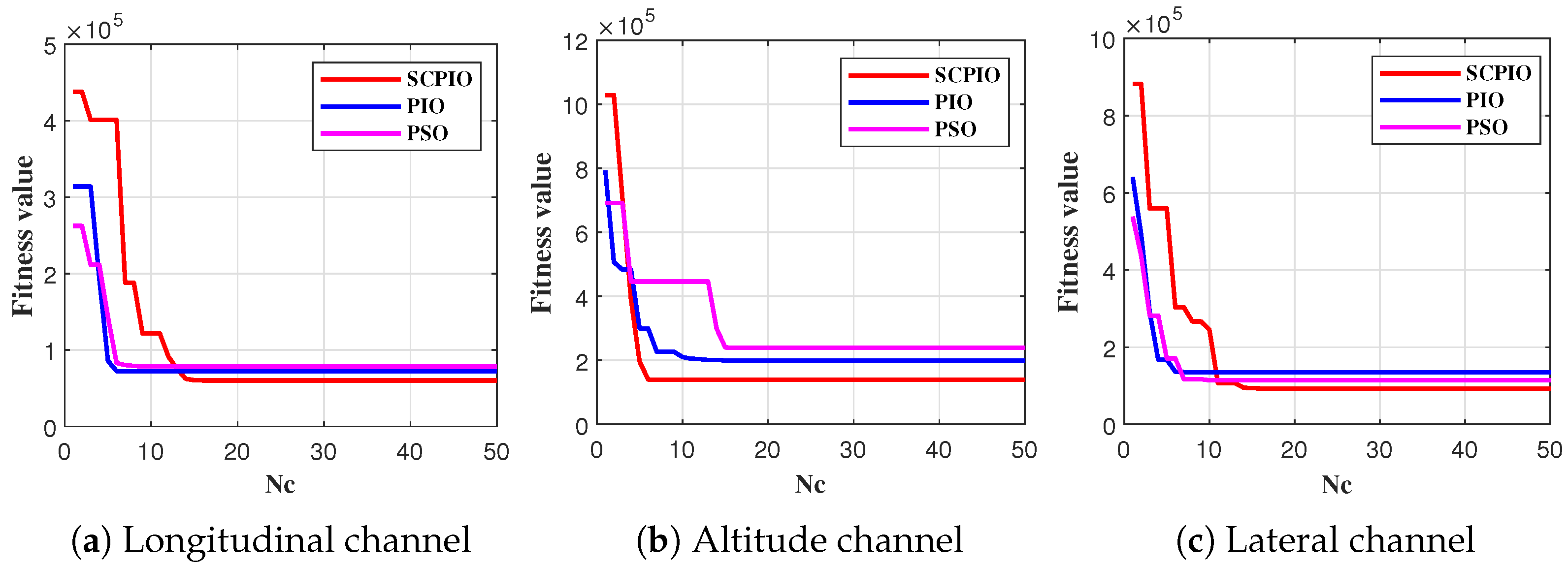
6.2. Implementation of Control System Optimization

Since the tracking and anti-disturbance performance of the designed robust control system depends on the control parameters of the control subsystem of each channel, the proposed SCPIO is used to search for their optimal values rather than a manual search. Then, the optimization results are compared to those of the standard PIO [22] and particle swarm optimization (PSO) [29] to validate the proposed SCPIO, which ensures the optimization of the control parameters. The parameters of each optimization algorithm are presented in

Table 1. Parameters of each optimization algorithm.

Algorithm	Parameter	Description	Value
PSO	$N_{C_{max}}$	Maximum iterative number	50
	$N_{PSO}$	Number of particles	100
	${\omega }_{PSO}$	Inertia weight	0.4
	$c_1$	Self-learning factor	2
	$c_2$	Group-learning factor	2
PIO, SCPIO	$N_{C_{1max}}^{pig}$	Iteration number of the map and compass operator	30
	$N_{C_{2max}}^{pig}$	Iteration number of the landmark operator	20
	$N^{pig}$	Number of pigeons	100
	R	Map and compass factor	0.4
	$[r_{min},r_{max}]$	Range of the control parameter of the sine map	[0.1, 0.9]

. Considering the amplitude range of the wake vortex effect and the response characteristics of the outer-loop position and the inner-loop attitude, the search sets of the observer bandwidths of the position and attitude loops are given as $\left\{{\omega }_{*(\ast =x_E,y_E,z_E)}\right|0<{\omega }_{*}<1\}$ and $\left\{{\omega }_{*(\ast =V,\theta ,\varphi ,\psi )}\right|5<{\omega }_{*}<10\}$, respectively. According to the expected dynamic characteristics of the control system, the controller gains are set to $k_{p_{*(\ast =x_E,z_E)}}\in [0.055,0.085]$, $k_{p_{y_E}}\in [0.01,0.04]$, and $k_{p_{*(\ast =\theta ,\varphi ,\psi )}}\in [0.7,1.4]$, $k_{p_V}\in [0.1,0.4]$, respectively. Note that the optimization of the control parameters is performed according to the divided channel. Furthermore, only the wake vortex effect of the corresponding channel is added to the UAV dynamic model in the optimization. The position and attitude weight coefficients of each channel are given as $k_{*(\ast =e_{x_E},\Delta V)}=1$, $k_{*(\ast =e_{z_E},\Delta \theta )}=1$ and $k_{e_{y_E}}=1$, $k_{\Delta \varphi }=10$, and $k_{\Delta \psi }=100$. The simulation termination time of the control system is set to $t_T=400$ s. Each optimization algorithm is run 10 times and the optimization result with the smallest fitness value was selected as the result of the optimization algorithm. The optimal values are presented in

Table 2. Optimal values of each optimization algorithm (The SCPIO algorithm and its optimized results are highlighted in bold).

Channel	Control Parameters	Algorithm	Optimal Values	Fitness Value
Longitudinal	$[K_{p_{x_E}},{\omega }_{x_E},K_{p_V},{\omega }_V]$	SCPIO	[0.0712, 0.11, 0.26, 6.12]	60,126
		PIO	[0.0634, 0.16, 0.23, 6.56]	72,151
		PSO	[0.0607, 0.20, 0.21, 6.81]	78,136
Altitude	$[K_{p_{z_E}},{\omega }_{z_E},K_{p_{\theta }},{\omega }_{\theta }]$	SCPIO	[0.06854, 0.71, 1.05, 8.21]	139,842
		PIO	[0.07345, 0.64, 1.16, 7.78]	199,774
		PSO	[0.07562, 0.61, 1.24, 7.46]	239,729
Lateral	$[K_{p_{y_E}},{\omega }_{y_E},K_{p_{\varphi }},{\omega }_{\varphi }$, $K_{p_{\psi }},{\omega }_{\psi }]$	SCPIO	[0.0254, 0.27, 0.98, 7.04, 1.10, 7.58]	93,251
		PIO	[0.0207, 0.30, 0.87, 7.43, 1.21, 7.42]	134,696
		PSO	[0.0318, 0.25, 1.25, 6.78, 1.00, 7.63]	113,974

and the evolution curves are illustrated in Figure 7. The proposed SCPIO has the strongest optimization ability, indicating that control parameters optimized with SCPIO can lead to the best performance of the control system in terms of tracking accuracy and rejection ability. By observing the optimal values of each optimization algorithm, a common phenomenon is apparent, that is, the bandwidths of the inner- and outer-loop extended-state observers of the altitude and lateral channels are larger than the bandwidth of the longitudinal channel. This indicates that the wake vortex effect is quite strong in these two channels.

In the robust close-formation control system based on a PI structure, the proposed SCPIO is also utilized to search for the optimal values of the control parameters to ensure that the comparison results are more fair and convincing. The fitness function of each channel and the parameters of the algorithm are the same as those of the designed control system. Similar to the above analysis and optimization process, the obtained optimal values are presented in

Table 3. Optimal values for the robust close-formation control system based on a PI structure.

Channel	Control Parameters	Algorithm	Optimal Values	Fitness Value
Longitudinal	$[K_{p_{x_E}}^{PI},K_{p_V}^{PI}]$	SCPIO	[0.1024, 250.7534]	28,146
Altitude	$[K_{p_{z_E}}^{PI},K_{i_{z_E}}^{PI},K_{p_{\theta }}^{PI}]$	SCPIO	[0.0021, 0.0005, 1.1568]	39,084
Lateral	$[K_{p_{y_E}}^{PI},K_{p_{\varphi }}^{PI},K_{p_{\psi }}^{PI}]$	SCPIO	[0.08791, 1.1326, 2.9736]	10,211

. Note that the fitness value of the lateral channel at the optimal position is less than those of the other two channels. This is because the optimal values of the control parameters can make the position and attitude accurately converge to the given command and initial state, respectively.

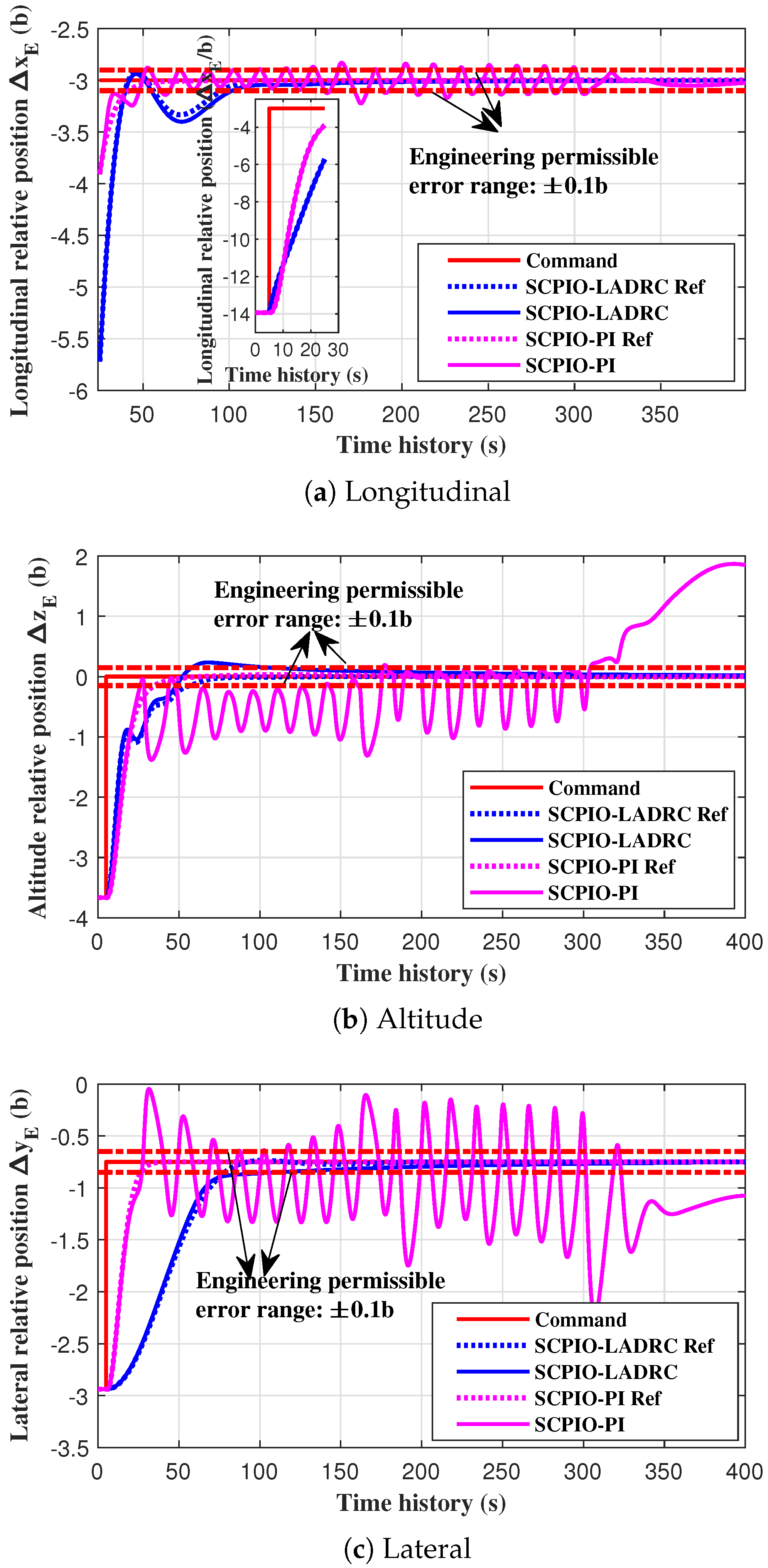
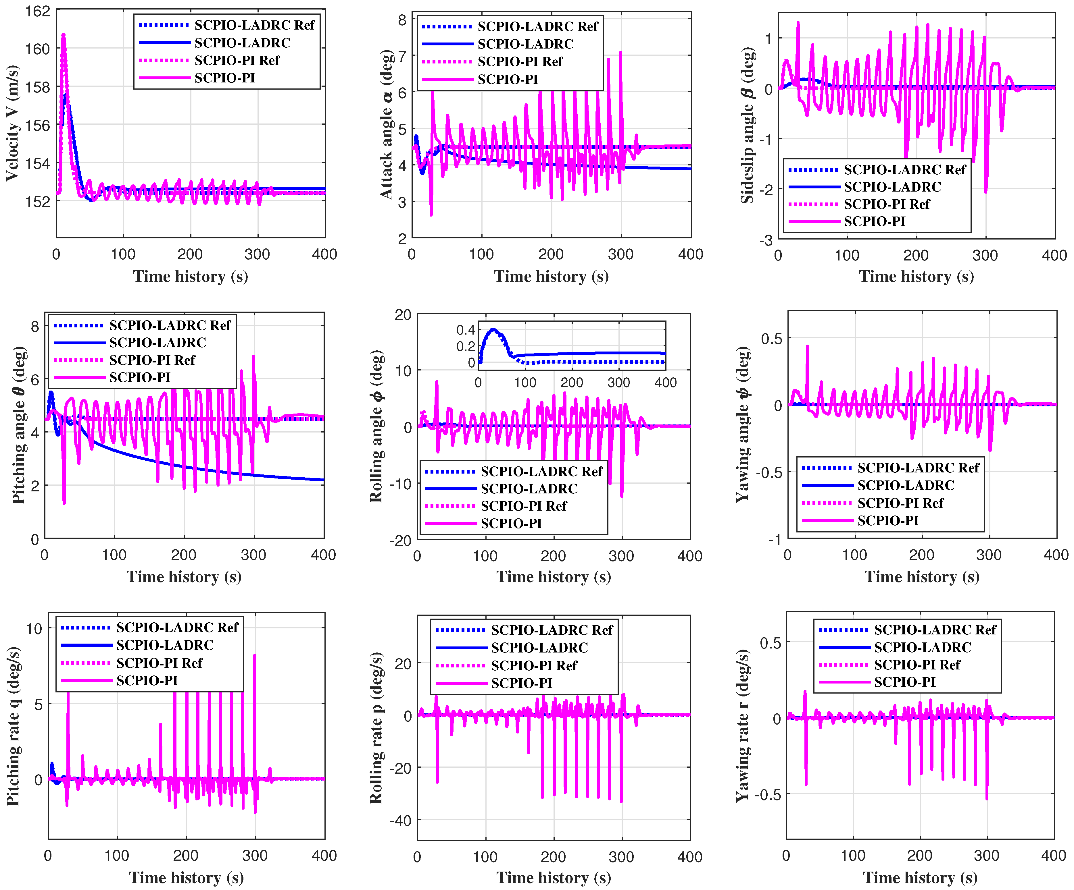
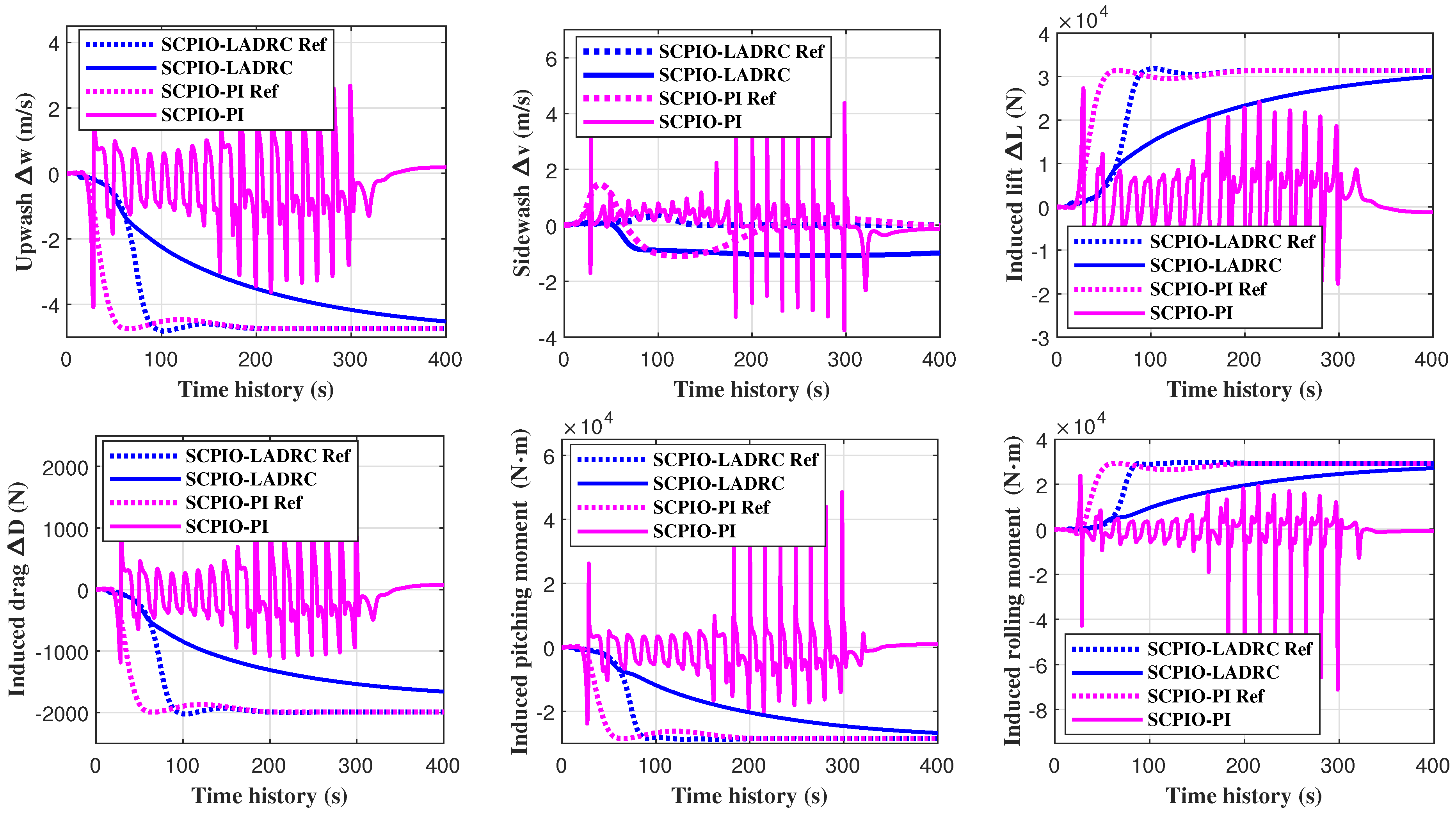
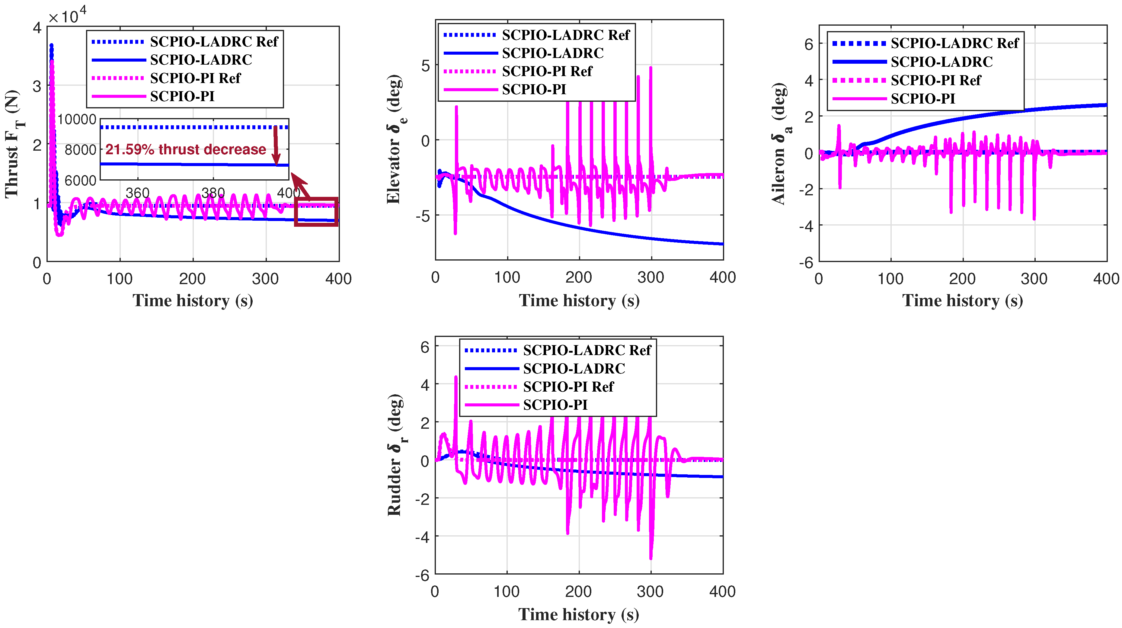
6.3. Tracking-Performance Validation

In order to validate the tracking performance of the designed robust close-formation control system under the wake vortex effect, two qualitative criteria are introduced, dynamic performance and stable performance. Furthermore, the tracking performance of the robust close-formation control system based on a PI structure under the wake vortex effect is also discussed for comparative analysis. On the other hand, the reference-tracking responses of the two control systems are generated without considering the wake vortex effect. Note that in the following demonstration of the simulation results, SCPIO-LADRC represents the proposed design and SCPIO-PI denotes the PI structure. SCPIO-LADRC Ref and SCPIO-PI Ref are the respective reference tracking responses.

The relative position tracking responses of the trailing UAV with respect to the leading UAV are demonstrated in Figure 8. The proposed design and the PI structure have almost the same reference-tracking responses. However, the dynamic performance of the PI structure deteriorates considerably when the wake vortex effect is added, indicating that the PI structure has almost no anti-disturbance ability. Even worse, the relative position not only significantly deviates from the sweet spot but also shows no sign of convergence at the end of the simulation. Compared to the PI structure, there is no significant difference between the tracking responses of the proposed design and its reference responses. This demonstrates the strong ability of the proposed design to suppress the disturbances caused by the wake vortex effect. Furthermore, it should also be noted that the dynamic performance of the proposed design deteriorates in terms of the setting time. For the expected control error of $\pm 0.1b$, however, the setting time increases slightly compared to that of the reference response. From the perspective of stable performance, the proposed design can guarantee that the relative position accurately converges to the sweet spot. On the other hand, the relative position components of the disturbed altitude and lateral channels under the PI structure have a large amplitude oscillation around the sweet spot. Therefore, these two channels need a high frequency for the extended-state observer, which further validates the optimization results of SCPIO.

The inner-loop state responses of the trailing UAV, including the velocity V, aerodynamic angles $\alpha$, $\beta$, attitude angles $\varphi$, $\theta$, $\psi$, and angular rates $p,q,r$, are illustrated in Figure 9. Similar to the results of the tracking responses, dynamic performance under the PI structure cannot be guaranteed. This is because the disturbances caused by the wake vortex effect can be divided into the induced forces acting on the outer-loop position subsystem and the induced moments acting on the inner-loop attitude subsystem. Owing to the induced moments, there are serious high-frequency oscillations and spikes in the inner-loop attitude subsystem. Furthermore, it should be noted that the poor inner-loop dynamic performance is a leading cause of the significant deterioration of the outer-loop dynamic performance. In contrast, the inner-loop state responses of the trailing UAV based on the proposed design exhibit smooth and stable convergence behavior. This means that the influences of the inner-loop disturbances on the dynamic performances are not transmitted to the outer loop. In conclusion, the LADRC controller is also used in the inner loop to form a cascade control system with the outer-loop LADRC controller, which can realize hierarchical suppression for the strong external disturbances caused by the wake vortex effect and significantly improve the tracking performance of the outer loop.

According to the established wake vortex model, the wake vortex effect can be considered a function of the relative position and attitude between the leading and trailing UAVs. If the trailing UAV has different tracking trajectories to converge to the sweet spot, the time histories of the wake vortex effect are also different, as shown in Figure 10. Under the control of the PI structure, the trailing UAV experienced more aggressive variations in the wake vortex effect. This is due to the fact the PI structure control has poor dynamic performance after being disturbed by the wake vortex effect, which makes the trailing UAV oscillate considerably around the sweet spot. The oscillations make the trailing UAV periodically fly through the downwash and upwash wake vortex regions, thereby inducing the more aggressive wake vortex effect. In turn, the more aggressive wake vortex effect can cause further deterioration in the control performance. The time responses of the control inputs under the two different control systems are shown in Figure 11. For the PI structure, severe control inputs are generated to counteract the disturbance of the more aggressive wake vortex effect as much as possible, which can cause actuator faults. However, through the proposed design, the disturbance of the wake vortex effect can be suppressed with less control effort. From the perspective of the control inputs, therefore, the proposed design is much more efficient than the PI structure. Furthermore, the proposed design leads to a $21.59\%$ decrease in the thrust input at the sweet spot, indicating that the trailing UAV could potentially save about $21.59\%$ of energy during close-formation flight.

7. Conclusions

In this paper, a robust close-formation control system with dynamic estimation and compensation is designed for UAV close-formation flight. The designed control system is divided into three control subsystems for the longitudinal, altitude, and lateral channels. The control subsystem of each channel is composed of two cascaded first-order LADRC controllers. One is responsible for the outer-loop position control and the other is used to stabilize the inner-loop attitude. This control system scheme can significantly reduce the coupling effect between channels and effectively suppress the transmission of the disturbance caused by the wake-vortex effect. A continuous-horseshoe vortex method with high estimation accuracy is employed to estimate the wake-vortex effect. The wake-vortex effect decreases significantly with the negative increase in the longitudinal position. Therefore, the longitudinal separation distance between the leading and trailing UAV should not exceed $10b$ if one wants to utilize the wake-vortex effect. The estimated wake-vortex effect is integrated into a nonlinear high-fidelity UAV model to describe the dynamic characteristics of the trailing UAV under the disturbance of the wake-vortex effect. SCPIO is utilized to simultaneously optimize the control parameters for the control subsystem of each channel, which can help the subsystem to achieve optimal performance. Compared to the conventional PI structure, the designed robust close-formation control system achieves error-bounded stable and robust dynamic performance. Furthermore, the control system follows the wake-vortex model with high estimation accuracy and the nonlinear high-fidelity UAV model, making it more suitable for engineering applications. In the future, engineering verification will be conducted to assess its practicality.

References

1. Zhan, G.; Gong, Z.; Lv, Q.; Zhou, Z.; Wang, Z.; Yang, Z.; Zhou, D. Flight Test of Autonomous Formation Management for Multiple Fixed-Wing UAVs Based on Missile Parallel Method. Drones 2022, 6, 99. [Google Scholar] [CrossRef]
2. Li, S.; Li, Y.; Zhu, J.; Liu, B. Predefined Location Formation: Keeping Control for UAV Clusters Based on Monte Carlo Strategy. Drones 2022, 7, 29. [Google Scholar] [CrossRef]
3. Xu, D.; Guo, Y.; Yu, Z.; Wang, Z.; Lan, R.; Zhao, R.; Xie, X.; Long, H. PPO-Exp: Keeping Fixed-Wing UAV Formation with Deep Reinforcement Learning. Drones 2022, 7, 28. [Google Scholar] [CrossRef]
4. Jiang, Y.; Bai, T.; Wang, Y. Formation Control Algorithm of Multi-UAVs Based on Alliance. Drones 2022, 6, 431. [Google Scholar] [CrossRef]
5. Luo, Y.; Bai, A.; Zhang, H. Distributed formation control of UAVs for circumnavigating a moving target in three-dimensional space. Guid. Navig. Control 2021, 1, 2150014. [Google Scholar] [CrossRef]
6. Zhang, Q.; Liu, H.H. Aerodynamics Modeling and Analysis of Close Formation Flight. J. Aircr. 2017, 54, 2192–2204. [Google Scholar] [CrossRef]
7. Kent, T.E.; Richards, A.G. Analytic Approach to Optimal Routing for Commercial Formation Flight. J. Guid. Control Dyn. 2015, 38, 1872–1884. [Google Scholar] [CrossRef]
8. Bangash, Z.A.; Sanchez, R.P.; Ahmed, A.; Khan, M.J. Aerodynamics of Formation Flight. J. Aircr. 2006, 43, 907–912. [Google Scholar] [CrossRef]
9. Hanson, C.E.; Pahle, J.; Reynolds, J.R.; Andrade, S.; Nelson, B. Experimental Measurements of Fuel Savings During Aircraft Wake Surfing. In Proceedings of the 2018 Atmospheric Flight Mechanics Conference, Atlanta, GA, USA, 25–29 June 2018. [Google Scholar]
10. Zhang, Q.; Liu, H.H. Aerodynamic Model-Based Robust Adaptive Control for Close Formation Flight. Aerosp. Sci. Technol. 2018, 79, 5–16. [Google Scholar] [CrossRef]
11. Zhang, Q.; Liu, H.H. UDE-Based Robust Command Filtered Backstepping Control for Close Formation Flight. IEEE Trans. Ind. Electron. 2018, 65, 8818–8827. [Google Scholar] [CrossRef]
12. Galzi, D.; Shtessel, Y. Closed-Coupled Formation Flight Control Using Quasi-Continuous High-Order Sliding-Mode. In Proceedings of the 2007 American Control Conference, New York, NY, USA, 9–13 July 2007. [Google Scholar]
13. Liu, C.; Jiang, B.; Zhang, K. Adaptive Fault-Tolerant H-Infinity Output Feedback Control for Lead–Wing Close Formation Flight. IEEE Trans. Syst. Man Cybern. Syst. 2020, 50, 2804–2814. [Google Scholar] [CrossRef]
14. Yuan, G.; Xia, J.; Duan, H. A Continuous Modeling Method via Improved Pigeon-Inspired Optimization for Wake vVortices in UAVs Close Formation Flight. Aerosp. Sci. Technol. 2022, 120, 107259. [Google Scholar] [CrossRef]
15. Han, J. From PID to Active Disturbance Rejection Control. IEEE Trans. Ind. Electron. 2009, 56, 900–906. [Google Scholar] [CrossRef]
16. Zhang, Y.; Chen, Z.; Zhang, X.; Sun, Q.; Sun, M. A Novel Control Scheme for Quadrotor UAV Based upon Active Disturbance Rejection Control. Aerosp. Sci. Technol. 2018, 79, 601–609. [Google Scholar] [CrossRef]
17. Ahi, B.; Nobakhti, A. Hardware Implementation of an ADRC Controller on a Gimbal Mechanism. IEEE Trans. Control Syst. Technol. 2018, 26, 2268–2275. [Google Scholar] [CrossRef]
18. Gao, Z. Scaling and Bandwidth-Parameterization Based Controller Tuning. In Proceedings of the American Control Conference, Minneapolis, MN, USA, July 2003; Available online: https://www.semanticscholar.org/paper/Scaling-and-bandwidth-parameterization-based-tuning-Gao/4f4d7b650767e01138a6969b97e5e2601779fb4c (accessed on 20 March 2023).
19. Zheng, Q.; Gaol, L.Q.; Gao, Z. On Stability Analysis of Active Disturbance Rejection Control for Nonlinear Time-Varying Plants with Unknown Dynamics. In Proceedings of the 46th IEEE Conference on Decision and Control, New Orleans, LA, USA, 12–14 December 2007. [Google Scholar]
20. Qi, Y.; Liu, J.; Yu, J. Dynamic Modeling and Hybrid Fireworks Algorithm-Based Path Planning of an Amphibious Robot. Guid. Navig. Control 2022, 2, 2250002. [Google Scholar] [CrossRef]
21. Zhu, K.; Han, B.; Zhang, T. Multi-UAV Distributed Collaborative Coverage for TargetSearch Using Heuristic Strategy. Guid. Navig. Control 2021, 1, 2150002. [Google Scholar] [CrossRef]
22. Duan, H.; Qiao, P. Pigeon-Inspired Optimization: A New Swarm Intelligence Optimizer for Air Robot Path Planning. Int. J. Intell. Comput. 2014, 7, 24–37. [Google Scholar] [CrossRef]
23. Tong, B.; Wei, C.; Shi, Y. Fractional Order Darwinian Pigeon-Inspired Optimization for Multi-UAV Swarm Controller. Guid. Navig. Control 2022, 2, 2250010. [Google Scholar] [CrossRef]
24. Duan, H.; Zhao, J.; Deng, Y.; Shi, Y.; Ding, X. Dynamic Discrete Pigeon-Inspired Optimization for Multi-UAV Cooperative Search-Attack Mission Planning. IEEE Trans. Aerosp. Electron. Syst. 2021, 57, 706–720. [Google Scholar] [CrossRef]
25. Huo, M.; Duan, H.; Fan, Y. Pigeon-Inspired Circular Formation Control for Multi-UAV System with Limited Target Information. Guid. Navig. Control 2021, 1, 2150004. [Google Scholar] [CrossRef]
26. Chen, K.; Zhou, F.; Liu, A. Chaotic Dynamic Weight Particle Swarm Optimization for Numerical Function Optimization. Knowl. Based Syst. 2018, 139, 23–40. [Google Scholar] [CrossRef]
27. Sonneveldt, L. Nonlinear F-16 Model Description; Delft University of Technology: Delft, The Netherlands, 2006. [Google Scholar]
28. Richard, S.R. Nonlinear F-16 Simulation Using Simulink and Matlab; University of Minnesota: Minneapolis, MN, USA, 2003. [Google Scholar]
29. Poli, R.; Kennedy, J.; Blackwell, T. Particle Swarm Optimization: An Overview. Swarm Intell. 2007, 1, 33–57. [Google Scholar] [CrossRef]
Figure 1. UAV close-formation flight.
Drones 07 00238 g001
Figure 2. Composition of the wake vortex.
Drones 07 00238 g002
Figure 3. General structure block of the first-order LADRC.
Drones 07 00238 g003
Figure 4. Overall scheme of the control system.
Drones 07 00238 g004
Figure 5. Sectional views of dimensionless velocity field induced by the wake vortex at different longitudinal positions.
Drones 07 00238 g005
Figure 6. Variation of the induced velocity with lateral and vertical position (x = −3b).
Drones 07 00238 g006
Figure 7. Evolution curves of each optimization algorithm.
Drones 07 00238 g007
Figure 8. Relative position tracking responses of the trailing UAV with respect to the leading UAV.
Drones 07 00238 g008
Figure 9. Velocity, aerodynamic angles, attitude angles, and attitude rate responses of the trailing UAV.
Drones 07 00238 g009
Figure 10. Time histories of the wake vortex effect experienced by the trailing UAV.
Drones 07 00238 g010
Figure 11. Time responses of the control inputs.
Drones 07 00238 g011