
Multi-Conflict-Based Optimal Algorithm for Multi-UAV Cooperative Path Planning


Abstract
:1. Introduction
- (1)
- Considering the constraint information of UAVs, the complex environment of multiple UAVs was modeled.
- (2)
- A sparse A * algorithm was designed to meet the flight constraints of UAVs, which reduces the search space and shortens the search time.
- (3)
- The collaborative conflict between multiple UAVs was defined; the priority of different collaborative conflicts is set; and the heuristic information was designed to guide the constraint tree to grow in the direction of conflict resolution to improve the algorithm’s convergence time.
2. Problem Description
2.1. Path Cost Analysis
2.1.1. Path Length Cost Function
2.1.2. Path Threat Cost Function
- (1)
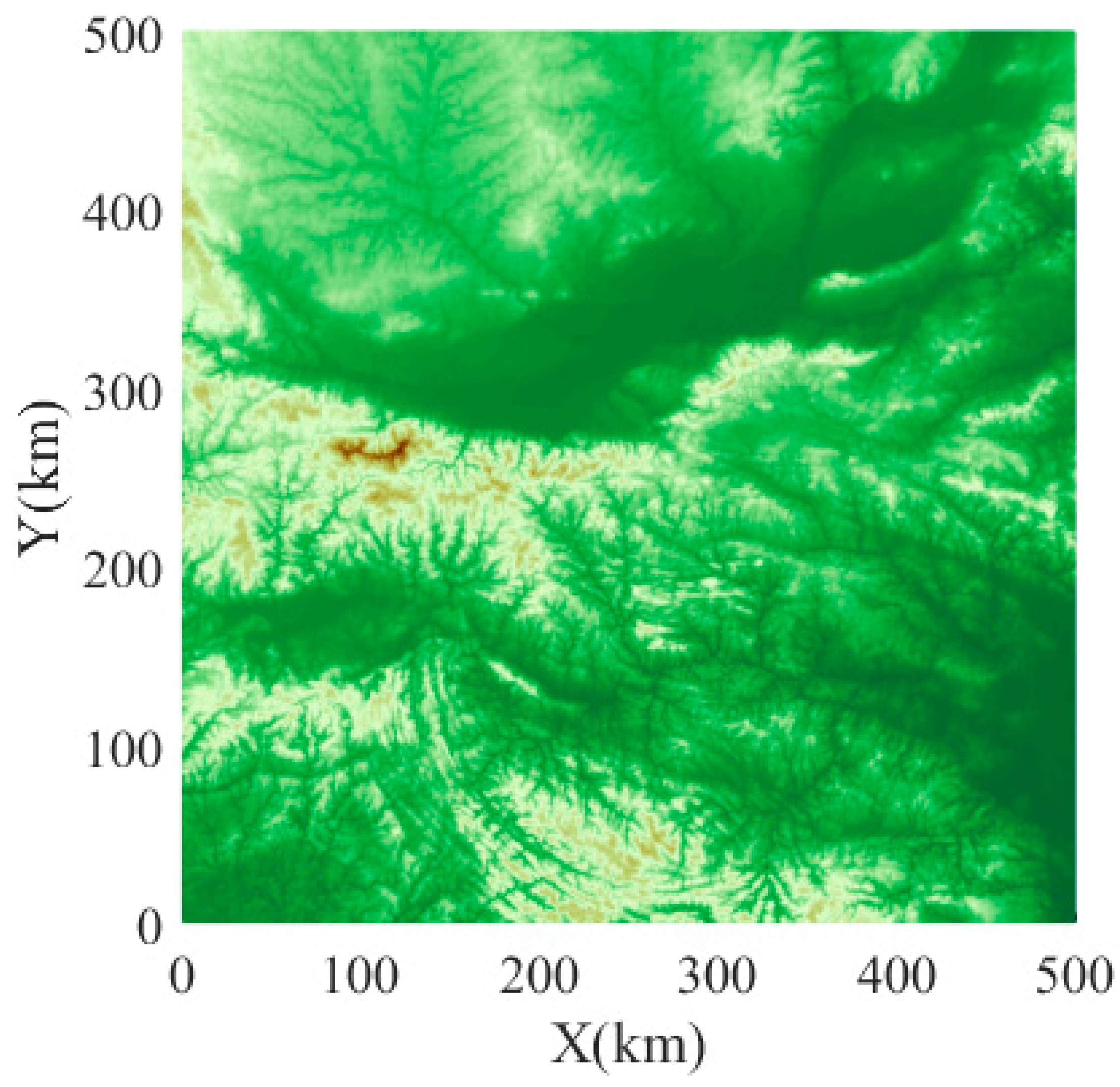
- Terrain threat model and cost analysis
- (2)
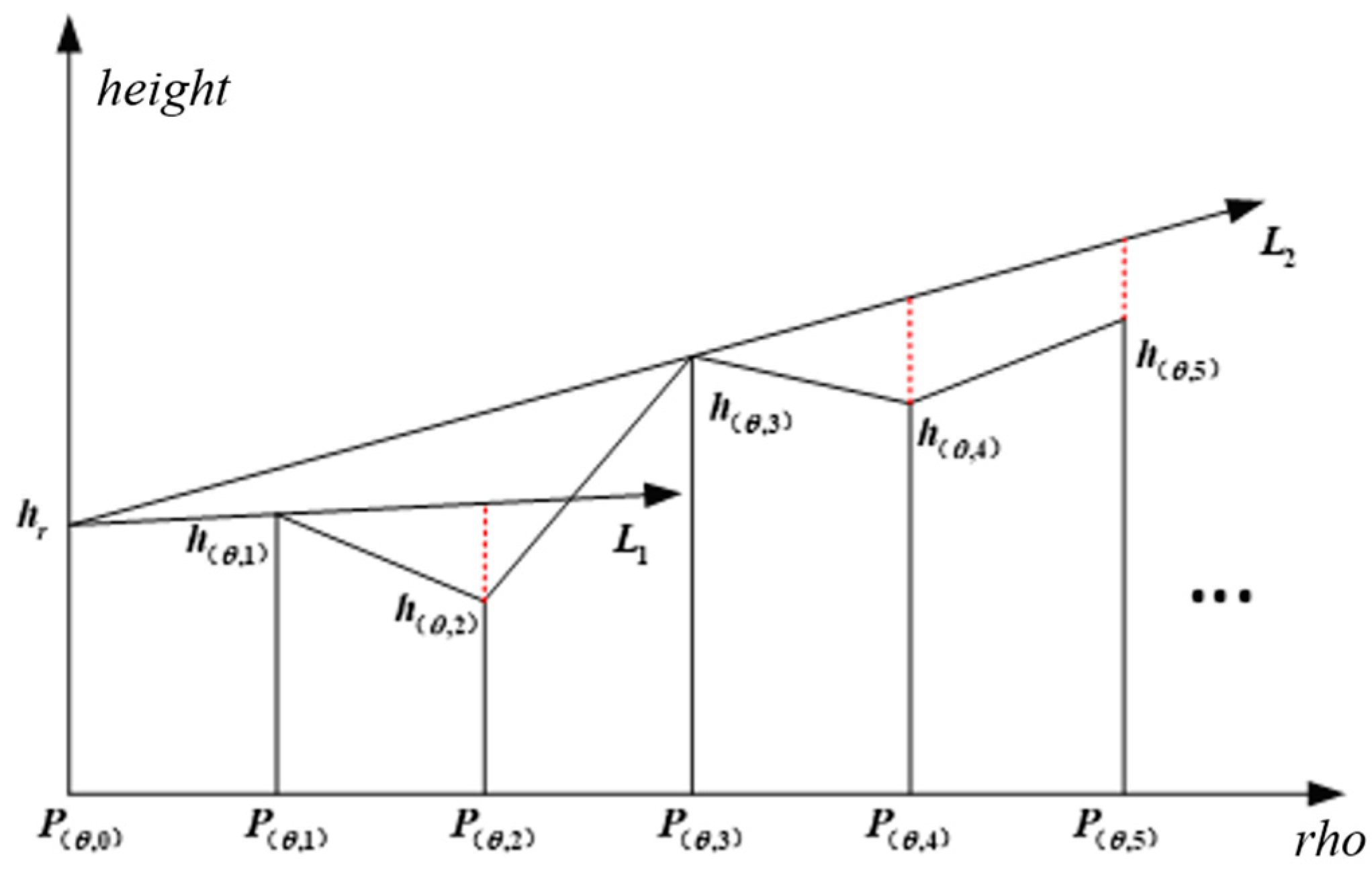
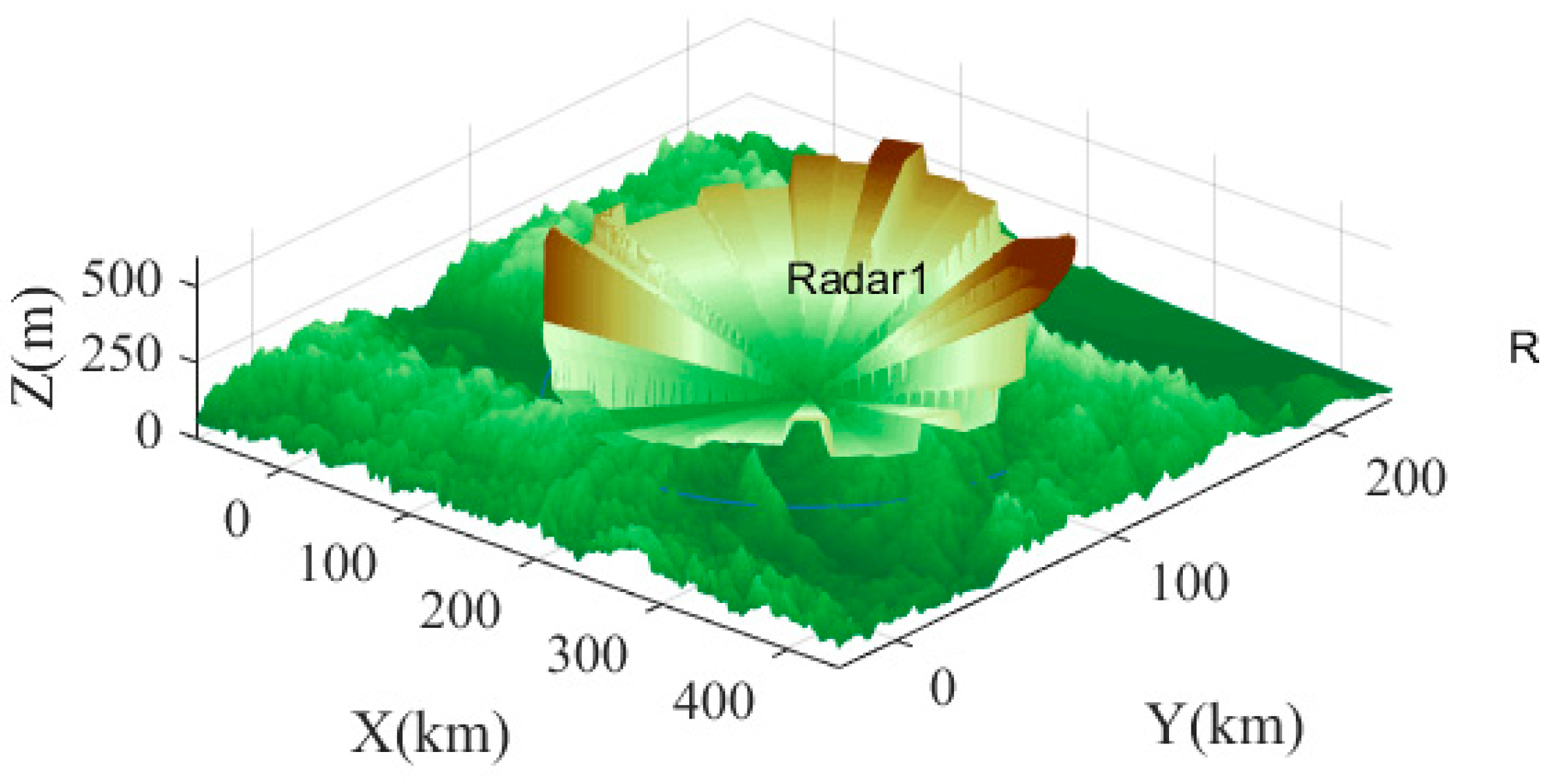
- Air defense radar model and analysis
- (a)
- Calculate the radar ray equation
- (b)
- Calculate the height of the radar blind spot
- (3)
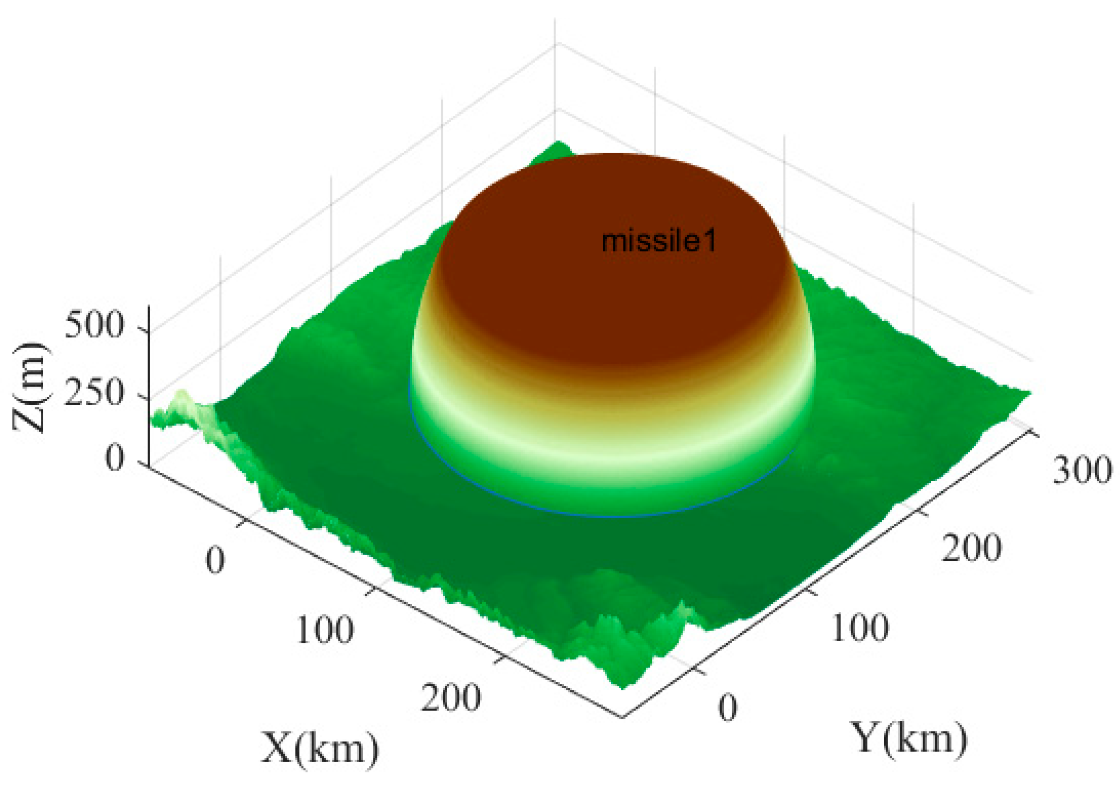
- Surface-to-air missile threat model and analysis
- (4)
- Anti-aircraft artillery threat model and analysis
- (5)
- No-fly zone threat model and analysis
2.2. Constraint Analysis
2.2.1. UAV Flight Constraint Analysis
- (1)
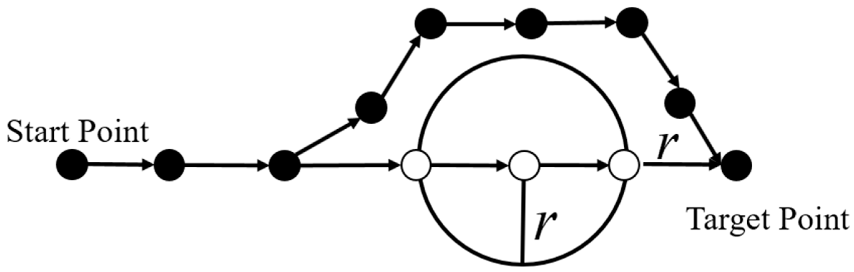
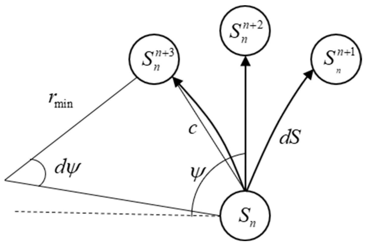
- Minimum turning radius
- (2)
- Minimum path segment length
- (3)
- Maximum path slope angle
- (4)
- Minimum ground height
2.2.2. Constraint Analysis
- (1)
- Time cooperative constraint analysis
- (2)
- Space cooperative constraint analysis
3. Multi-Conflict-Based Optimal Algorithm
3.1. Conflict Based Search
| Algorithm 1 Pseudocode of the CBS algorithm. |
| Input: MAPF instance ; Find path for each agent through A*; ; Insert into ; While Find the tree node with the minimal cost in ; if has conflicts, find the conflict which occurs first in ; Remove from ; for in : Create a new constraint set ; ; ; ; Find path for agent through A*; ; Insert into ; if does not have conflicts, . |
3.2. Algorithm Design of MCBS
3.2.1. High Level Search
- (1)
- Conflict detection and constraint generation
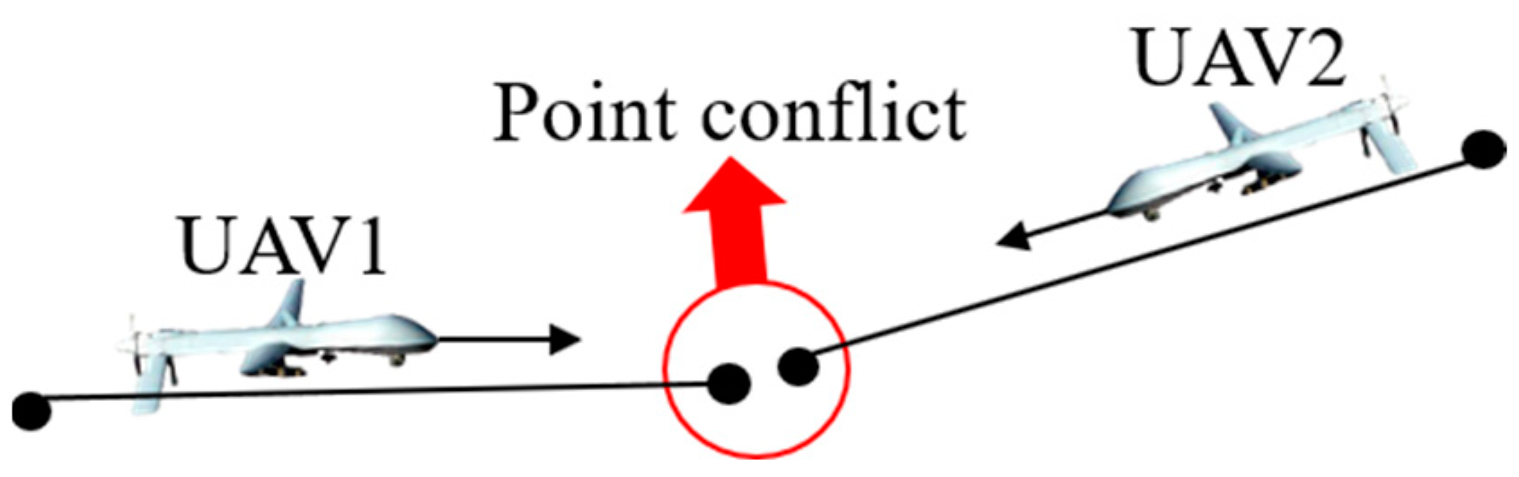
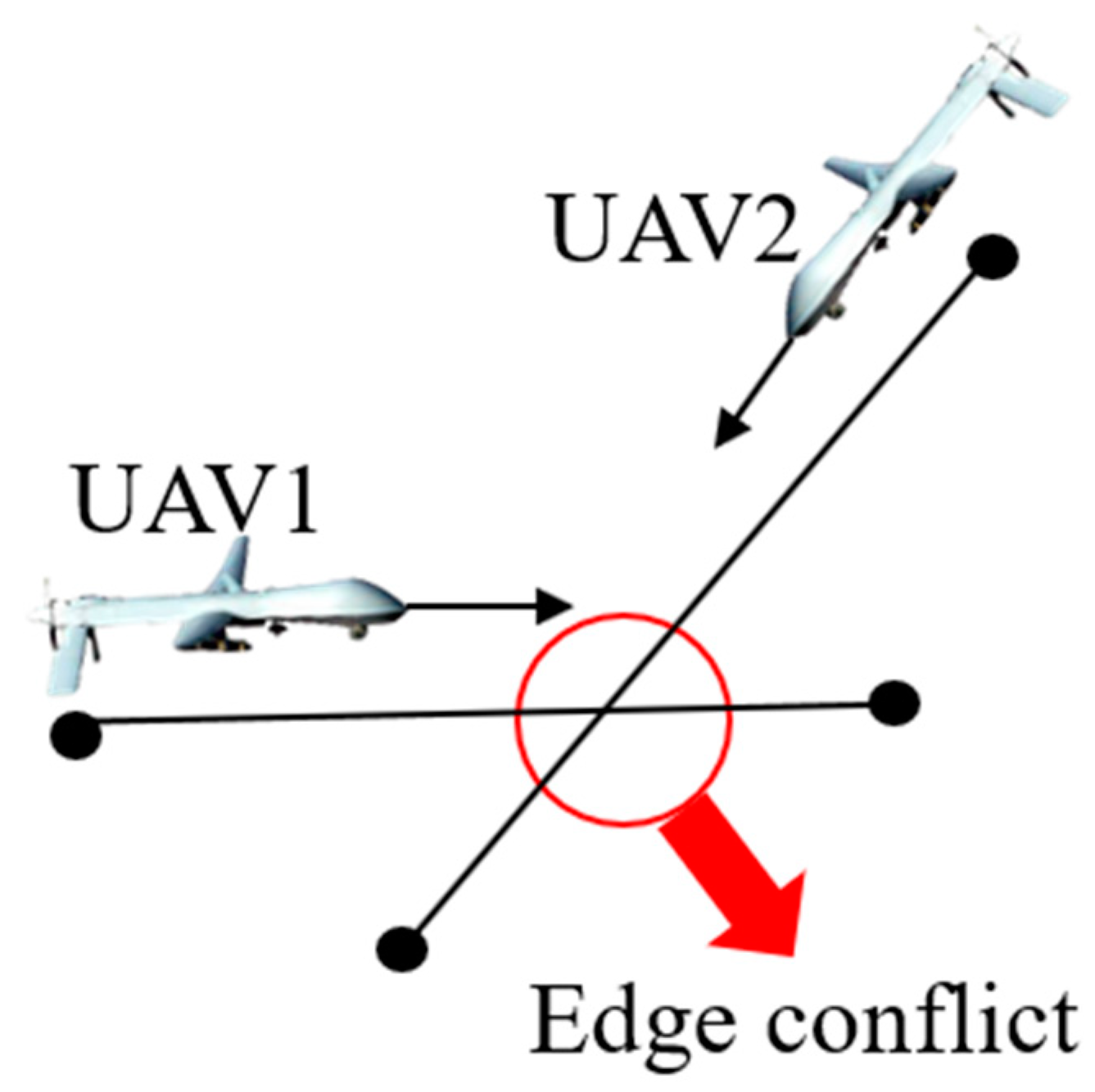
- (a)
- Space conflict
- (b)
- Time conflict
- (2)
- The constraint tree
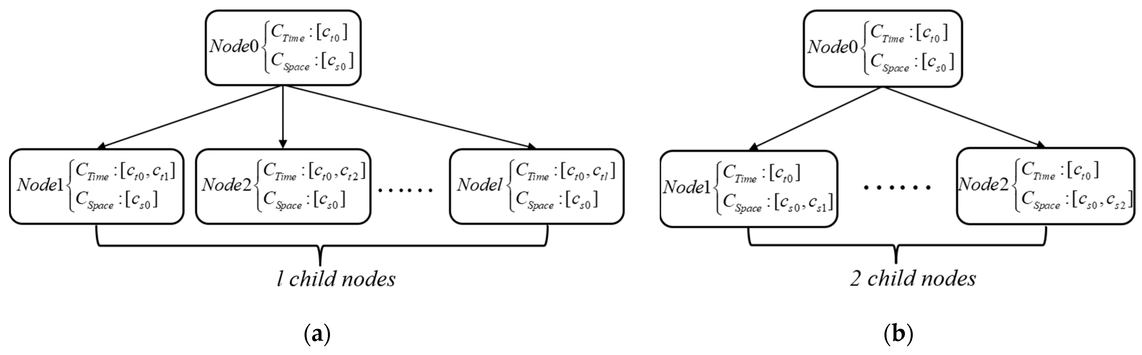
- (3)
- Create tree nodes
- (4)
- Tree node cost
- (5)
- Conflict resolution
3.2.2. Low Level Search
- (1)
- Waypoint cost function
- (2)
- Waypoint extension
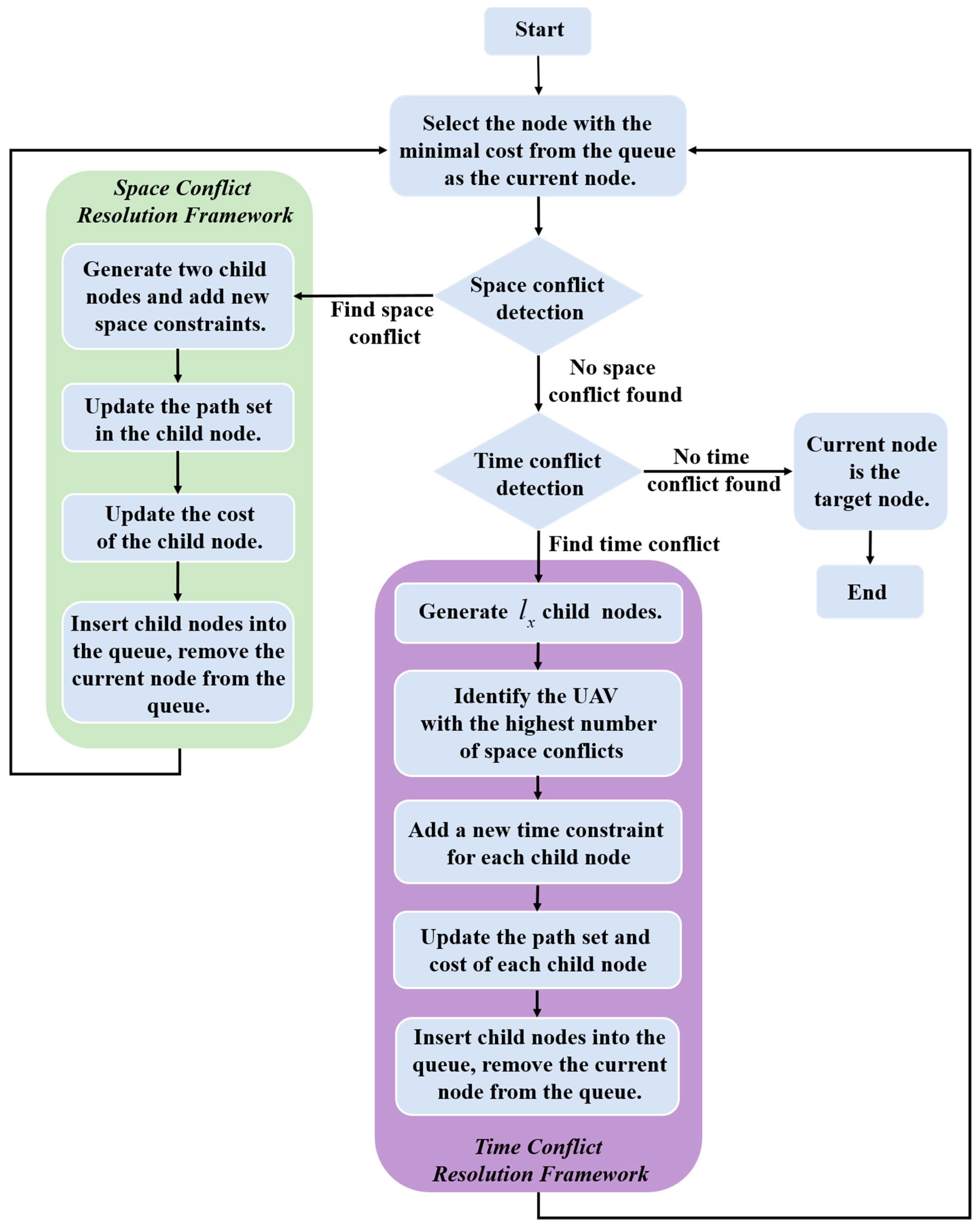
3.3. Algorithm Procedure
| Algorithm 2 Pseudocode of proposed algorithms. |
| Input: number of UAV, starting points, target points, , . Output: optimal solution that satisfies flight constraints and cooperative constraints. ; ; Find path for UAV through low level search; ; insert into ; while find the tree node with the minimal cost in ; if has space conflicts, find the space conflict which occurs first in ; remove from ; for in create a new space constraint set ; ; ; Find path for UAV through low level search; ; insert into ; if does not have space conflicts but has time conflicts , remove from ; for i = Create a new time constraint set ; ; ; ; ; Find path for UAV through low level search; ; insert into ; if has neither space conflicts nor time conflicts, ; then, . |
4. Simulation Studies
4.1. Environmental and Parametric
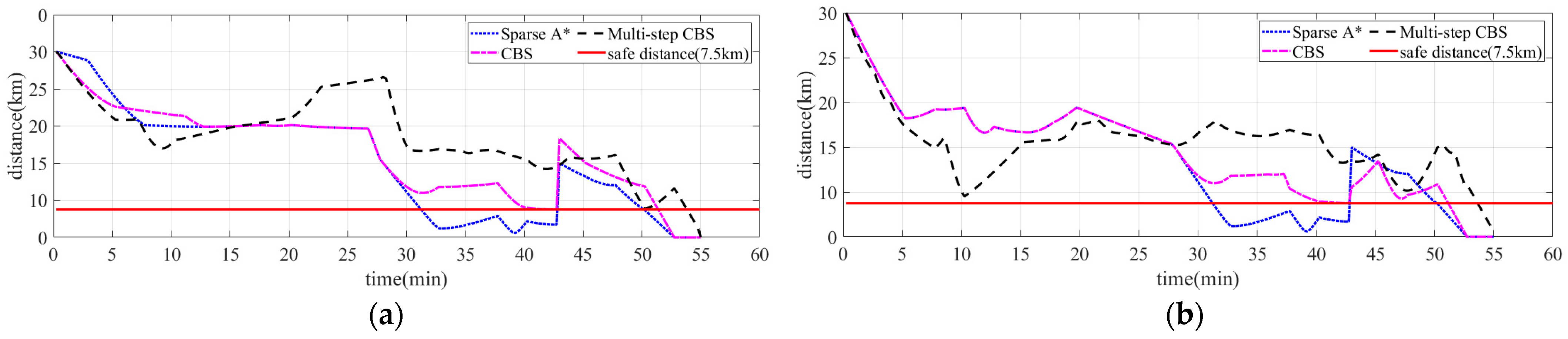
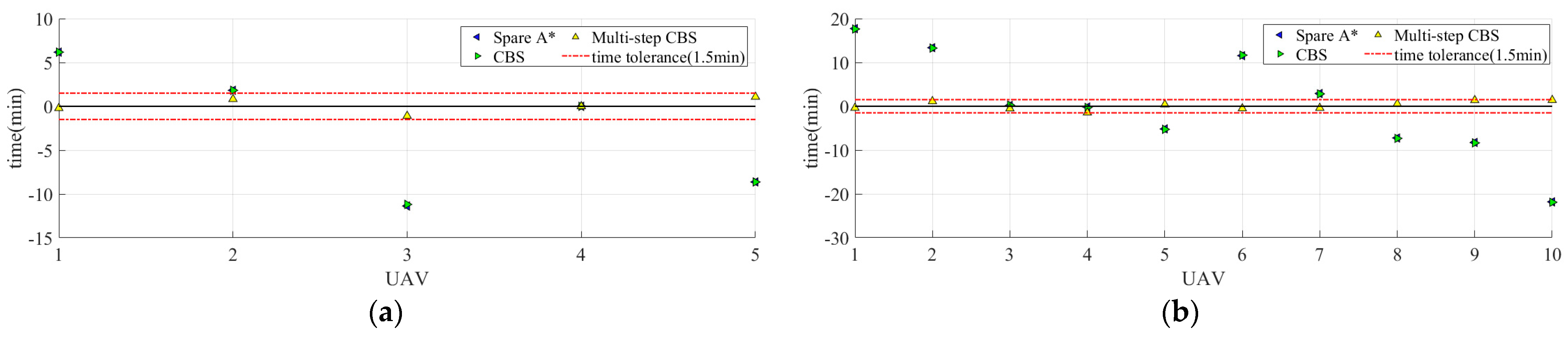
4.2. Algorithm Comparative Analysis
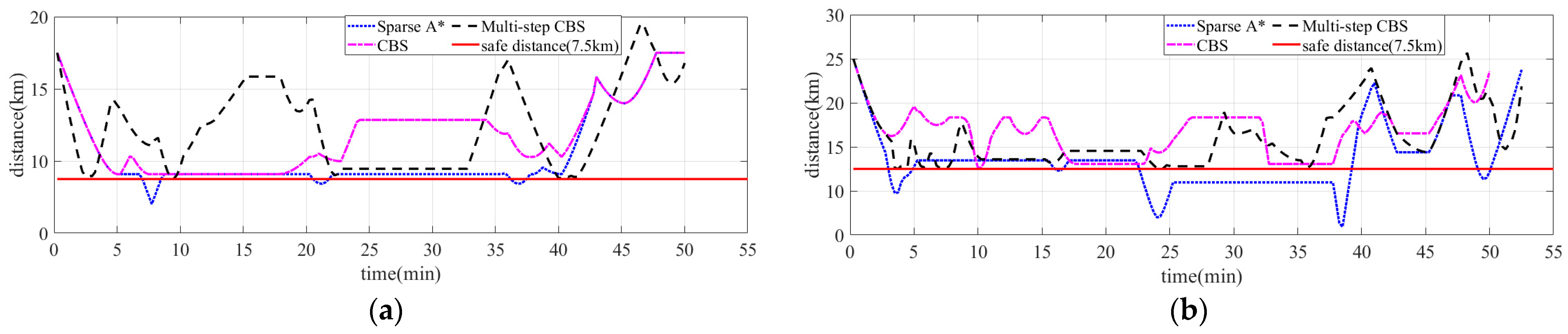
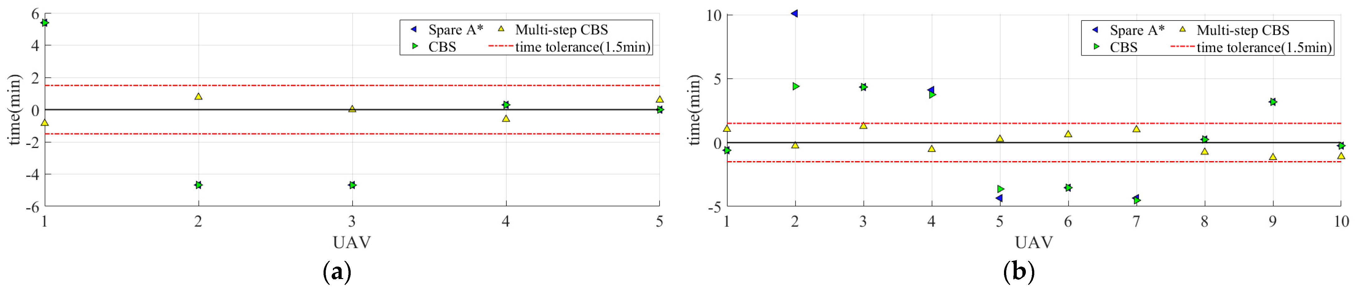
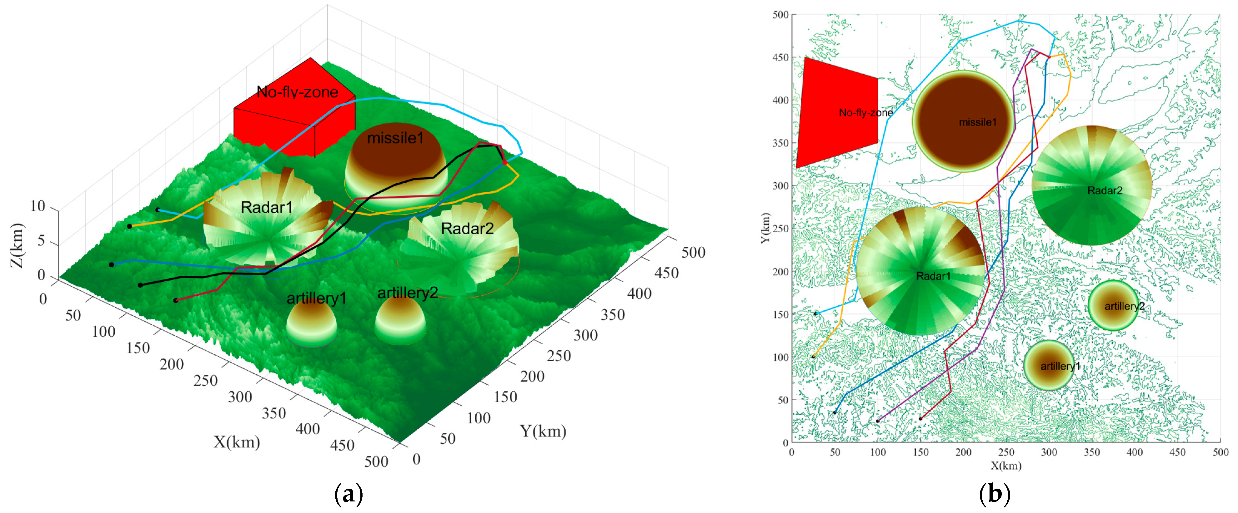
- (1)
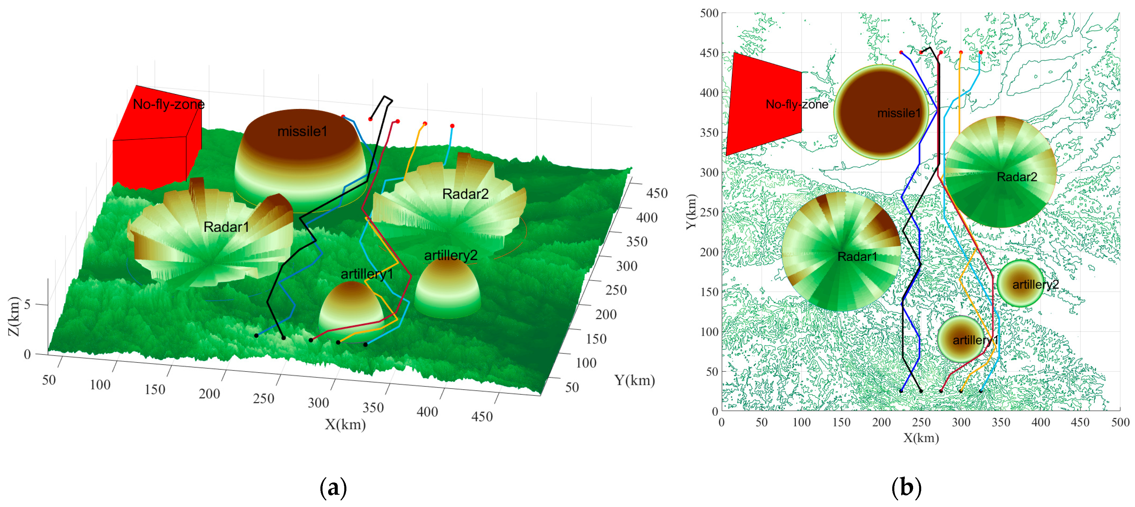
- Allocation task
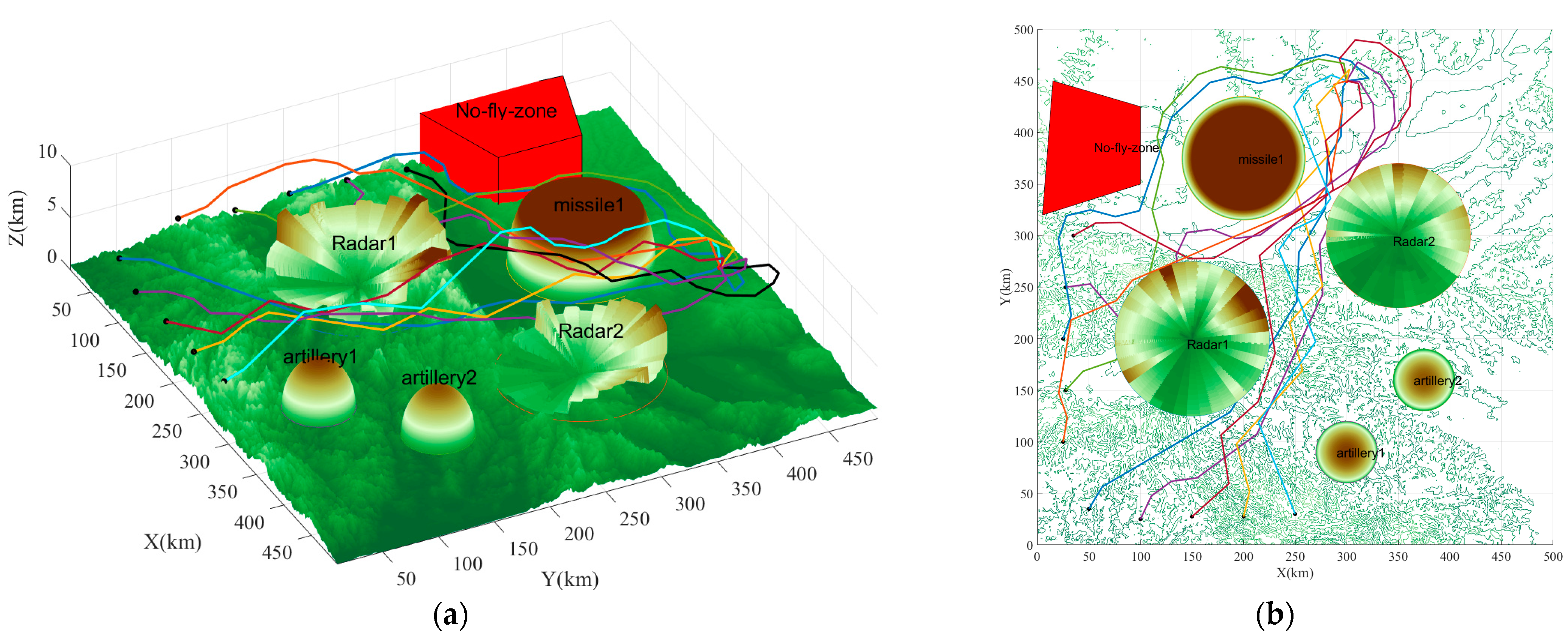
- (2)
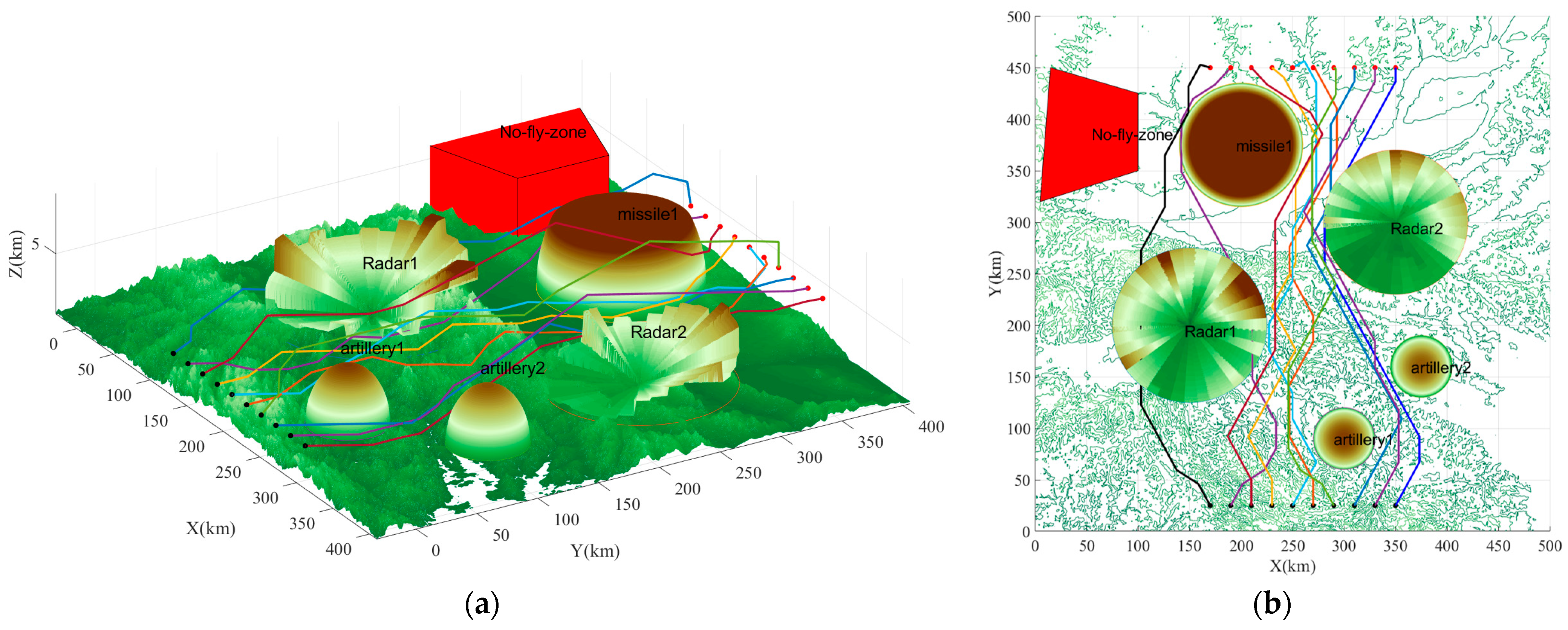
- Rendezvous task
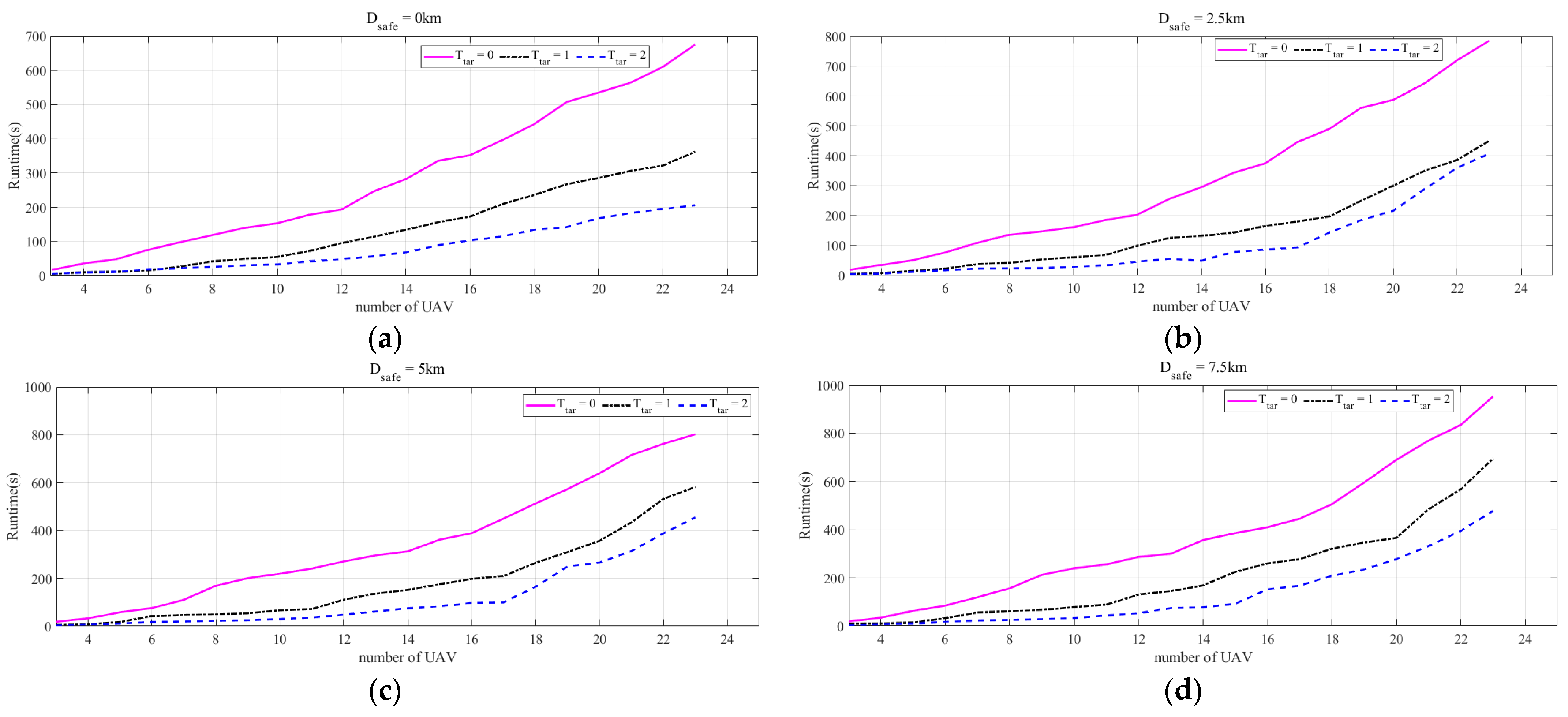
4.3. Parametric Analysis
4.3.1. Task Parameter Analysis
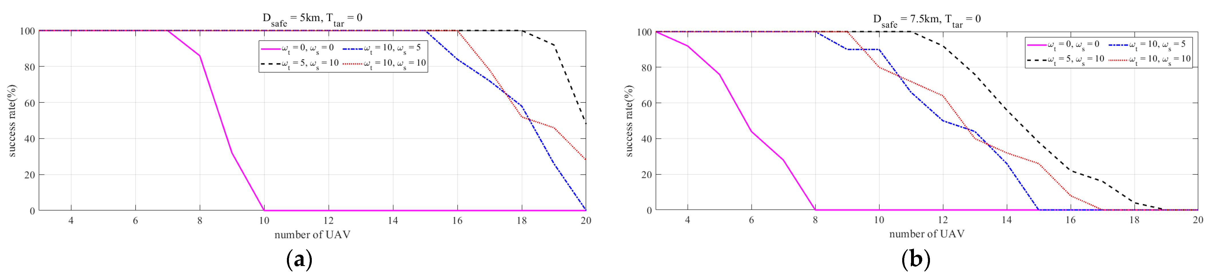
4.3.2. Penalty Factor Parameter Analysis
5. Conclusions
Author Contributions
Funding
Institutional Review Board Statement
Informed Consent Statement
Data Availability Statement
Acknowledgments
Conflicts of Interest
References
- Fu, B.; Chen, L.; Zhou, Y.; Zheng, D.; Wei, Z.; Dai, J.; Pan, H. An improved A* algorithm for the industrial robot path planning with high success rate and short length. Rob. Auton. Syst. 2018, 106, 26–37. [Google Scholar] [CrossRef]
- Gupta, L.; Jain, R.; Vaszkun, G. Survey of Important Issues in UAV Communication Networks. IEEE Commun. Surv. Tutorials 2016, 18, 1123–1152. [Google Scholar] [CrossRef] [Green Version]
- Patle, B.K.; Babu, L.G.; Pandey, A.; Parhi, D.R.K.; Jagadeesh, A. A review: On path planning strategies for navigation of mobile robot. Def. Technol. 2019, 15, 582–606. [Google Scholar] [CrossRef]
- Alpdemir, M.N. Tactical UAV path optimization under radar threat using deep reinforcement learning. Neural Comput. Appl. 2022, 34, 5649–5664. [Google Scholar] [CrossRef]
- Pan, Y.; Yang, Y.; Li, W. A Deep Learning Trained by Genetic Algorithm to Improve the Efficiency of Path Planning for Data Collection with Multi-UAV. IEEE Access 2021, 9, 7994–8005. [Google Scholar] [CrossRef]
- Ahmed, F.; Mohanta, J.C.; Keshari, A.; Yadav, P.S. Recent Advances in Unmanned Aerial Vehicles: A Review. Arab. J. Sci. Eng. 2022, 47, 7963–7984. [Google Scholar] [CrossRef] [PubMed]
- Roberge, V.; Tarbouchi, M.; Labonte, G. Comparison of parallel genetic algorithm and particle swarm optimization for real-time UAV path planning. IEEE Trans. Ind. Inform. 2013, 9, 132–141. [Google Scholar] [CrossRef]
- Majumder, S.; Prasad, M.S. Three dimensional D∗ algorithm for incremental path planning in uncooperative environment. In Proceedings of the 2016 3rd International Conference on Signal Processing and Integrated Networks (SPIN), Noida, India, 11–12 February 2016; pp. 431–435. [Google Scholar] [CrossRef]
- Dhawale, A.; Yang, X.; Michael, N. Reactive Collision Avoidance Using Real-Time Local Gaussian Mixture Model Maps. In Proceedings of the 2018 IEEE/RSJ International Conference on Intelligent Robots and Systems (IROS), Madrid, Spain, 1–5 October 2018; pp. 3545–3550. [Google Scholar] [CrossRef]
- Cap, M.; Novak, P.; Kleiner, A.; Selecky, M. Prioritized Planning Algorithms for Trajectory Coordination of Multiple Mobile Robots. IEEE Trans. Autom. Sci. Eng. 2015, 12, 835–849. [Google Scholar] [CrossRef] [Green Version]
- Damani, M.; Luo, Z.; Wenzel, E.; Sartoretti, G. PRIMAL2: Pathfinding Via Reinforcement and Imitation Multi-Agent Learning-Lifelong. IEEE Robot. Autom. Lett. 2021, 6, 2666–2673. [Google Scholar] [CrossRef]
- Van Den Berg, J.; Guy, S.J.; Lin, M.; Manocha, D. Reciprocal n-body collision avoidance. In Springer Tracts in Advanced Robotics; Springer: Berlin/Heidelberg, Germany, 2011. [Google Scholar]
- D’Amato, E.; Mattei, M.; Notaro, I. Distributed Reactive Model Predictive Control for Collision Avoidance of Unmanned Aerial Vehicles in Civil Airspace. J. Intell. Robot. Syst. Theory Appl. 2020, 97, 185–203. [Google Scholar] [CrossRef]
- Lalish, E.; Morgansen, K.A. Distributed reactive collision avoidance. Auton. Robots 2012, 32, 207–226. [Google Scholar] [CrossRef]
- Zu, C.; Yang, C.; Wang, J.; Gao, W.; Cao, D.; Wang, F.Y. Simulation and field testing of multiple vehicles collision avoidance algorithms. IEEE/CAA J. Autom. Sin. 2020, 7, 1045–1063. [Google Scholar] [CrossRef]
- Silver, D. Cooperative Pathfinding.pdf. In Proceedings of the AAAI Conference on Artificial Intelligence and Interactive Digital Entertainment, Marina Del Rey, CA, USA, 1–2 June 2005; pp. 117–122. [Google Scholar]
- Tai, R.; Wang, J.; Chen, W. A prioritized planning algorithm of trajectory coordination based on time windows for multiple AGVs with delay disturbance. Assem. Autom. 2019, 39, 753–768. [Google Scholar] [CrossRef]
- Cap, M.; Novak, P.; Selecky, M.; Faigl, J.; Vokffnek, J. Asynchronous decentralized prioritized planning for coordination in multi-robot system. In Proceedings of the 2013 IEEE/RSJ International Conference on Intelligent Robots and Systems, Tokyo, Japan, 3–7 November 2013; pp. 3822–3829. [Google Scholar] [CrossRef]
- Liu, Z.; Wei, H.; Wang, H.; Li, H.; Wang, H. Integrated Task Allocation and Path Coordination for Large-Scale Robot Networks With Uncertainties. IEEE Trans. Autom. Sci. Eng. 2022, 19, 2750–2761. [Google Scholar] [CrossRef]
- Panescu, D.; Pascal, C. A constraint satisfaction approach for planning of multi-robot systems. In Proceedings of the 2014 18th Int. Conf. Syst. Theory, Control Comput. ICSTCC 2014, Sinaia, Romania, 17–19 October 2014; pp. 157–162. [Google Scholar] [CrossRef]
- Sharon, G.; Stern, R.; Felner, A.; Sturtevant, N.R. Conflict-based search for optimal multi-agent pathfinding. Artif. Intell. 2015, 219, 40–66. [Google Scholar] [CrossRef]
- Tinka, A.; Durham, J.W.; Koenig, S. Lifelong Multi-Agent Path Finding in Large-Scale Warehouses Extended Abstract. In Proceedings of the AAAI Conference on Artificial Intelligence, New York, NY, USA, 7–12 February 2020; pp. 1–3. [Google Scholar]
- Semiz, F.; Polat, F. Incremental multi-agent path finding. Futur. Gener. Comput. Syst. 2021, 116, 220–233. [Google Scholar] [CrossRef]
- Barer, M.; Sharon, G.; Stern, R.; Felner, A. Suboptimal variants of the conflict-based search algorithm for the multi-agent pathfinding problem. In Proceedings of the International Symposium on Combinatorial Search, Prague, Czech Republic, 15–17 August 2014; pp. 19–27. [Google Scholar] [CrossRef]
- Li, J.; Ruml, W.; Koenig, S. EECBS: A Bounded-Suboptimal Search for Multi-Agent Path Finding. AAAI Conf. Artif. Intell. AAAI 2021, 14A, 12353–12362. [Google Scholar] [CrossRef]
- Bayerlein, H.; Theile, M.; Caccamo, M.; Gesbert, D. Multi-UAV Path Planning for Wireless Data Harvesting with Deep Reinforcement Learning. IEEE Open J. Commun. Soc. 2021, 2, 1171–1187. [Google Scholar] [CrossRef]
- Zhang, Z.; Wu, J.; Dai, J.; He, C. A Novel Real-Time Penetration Path Planning Algorithm for Stealth UAV in 3D Complex Dynamic Environment. IEEE Access 2020, 8, 122757–122771. [Google Scholar] [CrossRef]
- Xu, C.; Xu, M.; Yin, C. Optimized multi-UAV cooperative path planning under the complex confrontation environment. Comput. Commun. 2020, 162, 196–203. [Google Scholar] [CrossRef]
- Yang, P.; Tang, K.; Lozano, J.A.; Cao, X. Path Planning for Single Unmanned Aerial Vehicle by Separately Evolving Waypoints. IEEE Trans. Robot. 2015, 31, 1130–1146. [Google Scholar] [CrossRef] [Green Version]
- Besada-Portas, E.; De La Torre, L.; De La Cruz, J.M.; De Andrés-Toro, B. Evolutionary trajectory planner for multiple UAVs in realistic scenarios. IEEE Trans. Robot. 2010, 26, 619–634. [Google Scholar] [CrossRef]


| Type of Threat | Attributes | |||
|---|---|---|---|---|
| Air defense radar | radar number | coordinates | radius | |
| radar 0 | [300, 400, 20] | 80 km | ||
| radar 1 | [700, 600, 25] | 70 km | ||
| Surface-to-air missile | missile number | coordinates | radius | |
| missile 0 | [400, 750, 20] | 60 km | ||
| Anti-aircraft artillery | artillery number | coordinates | radius | |
| artillery 0 | [600, 180, 25] | 30 km | ||
| artillery 1 | [750, 320, 20] | 30 km | ||
| No-fly zone | vertex coordinates: | |||
| p1 = [520, 320]; | p2 = [620, 340]; | |||
| p3 = [600, 430]; | p4 = [520, 430]; | |||
| Allocation Task | Rendezvous Task | |
|---|---|---|
| Safe distance | 7.5 km | 7.5 km |
| Maximum node difference | 0 | 0 |
| Minimum unit step | 25 km | 25 km |
| Minimum turning radius | 25 km | 25 km |
| Minimum ground height | 2.5 km | 2.5 km |
| Sparse A* | CBS | MCBS | |
|---|---|---|---|
| Minimum unit step of the paths | 25.57 km | 25.36 km | 25.11 km |
| Minimum turning radius of the paths | 25.54 km | 25.38 km | 25.21 km |
| Minimum ground height of the paths | 3.62 km | 3.62 km | 2.97 km |
| Maximum node difference of the paths | 4 | 4 | 0 |
| Shortest distance of the paths | 0.93 km | 7.60 km | 7.51 km |
| Maximum time tolerance of the paths | 10.10 min | 4.52 min | 1.26 min |
| Sparse A* | CBS | MCBS | |
|---|---|---|---|
| Minimum unit step of the paths | 25.31 km | 25.31 km | 25.15 km |
| Minimum turning radius of the paths | 25.85 km | 25.85 km | 25.31 km |
| Minimum ground height of the paths | 3.86 km | 3.86 km | 3.1 km |
| Maximum node difference of the paths | 4 | 4 | 0 |
| Shortest distance of the paths | 1.20 km | 7.52 km | 9.02 km |
| Maximum time tolerance of the paths | 21.90 min | 21.90 min | 1.40 min |
Disclaimer/Publisher’s Note: The statements, opinions and data contained in all publications are solely those of the individual author(s) and contributor(s) and not of MDPI and/or the editor(s). MDPI and/or the editor(s) disclaim responsibility for any injury to people or property resulting from any ideas, methods, instructions or products referred to in the content. |
© 2023 by the authors. Licensee MDPI, Basel, Switzerland. This article is an open access article distributed under the terms and conditions of the Creative Commons Attribution (CC BY) license (https://creativecommons.org/licenses/by/4.0/).
Share and Cite
Liu, X.; Su, Y.; Wu, Y.; Guo, Y. Multi-Conflict-Based Optimal Algorithm for Multi-UAV Cooperative Path Planning. Drones 2023, 7, 217. https://doi.org/10.3390/drones7030217
Liu X, Su Y, Wu Y, Guo Y. Multi-Conflict-Based Optimal Algorithm for Multi-UAV Cooperative Path Planning. Drones. 2023; 7(3):217. https://doi.org/10.3390/drones7030217
Chicago/Turabian StyleLiu, Xiaoxiong, Yuzhan Su, Yan Wu, and Yicong Guo. 2023. "Multi-Conflict-Based Optimal Algorithm for Multi-UAV Cooperative Path Planning" Drones 7, no. 3: 217. https://doi.org/10.3390/drones7030217