Article

Lane Level Positioning Method for Unmanned Driving Based on Inertial System and Vector Map Information Fusion Applicable to GNSS Denied Environments

1
School of Instrumentation and Optoelectronic Engineering, Beihang University, Beijing 100191, China
2
Beijing Institute of Spacecraft System Engineering, CAST, Beijing 100076, China
3
School of Materials Science and Engineering, Hubei University, Wuhan 430062, China
*
Author to whom correspondence should be addressed.
Drones 2023, 7(4), 239; https://doi.org/10.3390/drones7040239
Submission received: 10 February 2023 / Revised: 25 March 2023 / Accepted: 27 March 2023 / Published: 29 March 2023

Abstract

:
With the development of vehicle sensors, unmanned driving has become a research hotspot. Positioning is also considered to be one of the most challenging directions in this field. Aiming at the poor positioning accuracy of vehicles under GNSS denied environments, a lane-level positioning method based on inertial system and vector map information fusion is proposed. A dead reckoning model based on optical fiber IMU and odometer is established, and its positioning error is regarded as a priori information. Furthermore, a map matching model based on HMM is built up. Three validation experiments are carried out and experimental results show that the positioning error can be reduced to less than 30 cm when driving for about 7 min, which proves the effectiveness of the proposed method. Our work may provide a reference for the further improvement of positioning for unmanned driving under GNSS denied environments.

1. Introduction

Unmanned driving technology has become a research hotspot with the development and mass production of on-board sensors, which means that the vehicle can carry out motion control by itself according to its own perception and understanding of the surrounding environmental conditions, and reach the level of a human driver [1]. In order to determine the position of the vehicle in the environment, the positioning module plays a very important role in autonomous driving [2,3]. Traditional inertial navigation methods, one of whose typical combinations is IMU (inertial measurement unit) and odometer can achieve high-precision positioning in GNSS (Global Navigation Satellite System) denied environment, but working for a long time will lead to error accumulation [4,5,6]. To solve this problem, an integrated positioning method using other information to assist inertia is proposed. Table 1 summarizes some representative integrated positioning methods.
In order to promote positioning accuracy, the integrated positioning method based on SINS/OD (Odometer) is proposed. However, it can only slow down the speed of error accumulation, but cannot eliminate errors. Furthermore, in order to suppress the divergence of the altitude channel, the integrated positioning method based on SINS/Altimeter is proposed, but it still has low accuracy. Moreover, magnetic information is introduced to improve the positioning accuracy so that the integrated positioning method based on SINS/GMNS (Geomagnetic Matching Navigation System) has been developed. It can work in all weather and its positioning error would not accumulate over time, but it is sensitive to external magnetic field and has low reliability. In addition, the integrated positioning method based on SINS/SMNS (Scene Matching Navigation System) also has been proposed, which has the advantages of low cost and no accumulated positioning error. However, it is difficult to collect the database and it is vulnerable to weather. Furtherly, the inertial/visual integrated positioning method derived from this does not have the problem of database collection, and it can achieve the mapping of the environment at the same time, which is currently a research hotspot [13]. However, its computational complexity is large, and it is still affected by the environment, which is not conducive to large-scale promotion and application [14]. Beyond that, common sensors including lidar, camera and millimeter wave radar have also been adopted [15,16,17,18,19,20,21]. Nevertheless, these schemes are easily affected by the environment, resulting in larger error of positioning results [22]. As a consequence, it is essential to seek an active positioning method that is not affected by the external environment.
As a priori information, a vector map can provide position reference for an inertial positioning system and is a very good auxiliary means [23]. With the development of technology, digital maps become easy to obtain and store. Therefore, the integrated positioning method based on inertial technology and map information fusion has great application prospects in scenes such as underground parking lots and large-scale logistics complex areas.
Positioning based on map matching is also a mainstream method of vehicle positioning in the absence of satellite signal [24,25]. According to different reference information, it can be divided into three categories: based on geometry, based on probability statistics and based on road topology. Geometry-based methods can mainly be divided into three types: point to point [26], point to line [27] and line to line [28]. The representative work includes: Zeng et al. [29] proposed a method to describe the proximity of road network and trajectory by curvature integral value. The similarity function of two adjacent GPS points and corresponding candidate road segments was calculated according to the set rules, and the proximity between them was regarded as the criterion of map matching. Sharma et al. [30] restored the real track route of the vehicle through the GPS trajectory data. The Fréchet distance was used to denote the matching degree between the GPS point trajectory and the road network [31]. However, the positioning accuracy of this method was 5.5 m, which could not meet the needs of automatic driving.
Probability statistics-based methods give a certain probability value to each candidate road segment through self-designed rules, so as to determine the optimal matching road segment [32,33]. The representative work includes the following: Ochieng et al. [34] came up with an improved probabilistic map matching algorithm to balance the inaccurate positioning data and digital map data. The algorithm considered the error sources related to the positioning sensors, the historical trajectory of the vehicle, the topology information of the road network and the heading and speed information of the vehicle, and used the probabilistic statistical method to identify the real road segment of the vehicle. Yue et al. [35] proposed a cooperative probabilistic semantic map matching method to realize semantic perception and cooperative localization. Semantic perception, probabilistic data association and nonlinear model linearization were completed in an integrated framework. A probabilistic semantic data association algorithm based on expectation maximization was put forward. The test results in the public dataset showed that the method had good robustness and accuracy.
Road topology-based methods mainly limit the number of candidate road segments corresponding to each sampled point by using the historical sampled point parameters, vehicle speed and the topological relationship of spatial road network. The representative work includes the following: Quddus et al. [36] proposed an improved weighted topology matching algorithm, which combined the weights of factors such as heading, projection distance and correlation between segments, and selected the optimal segment with the largest weight by calculating the weight of each sampled point and candidate segment. However, the algorithm did not take the historical location point data into account, so the matching and positioning accuracy were not high. Velaga et al. [37] came up with a map matching algorithm based on weighted topology on the basis of Quddus’s work, taking the two factors of curve restriction and road connectivity into account. The algorithm had high matching accuracy in simple urban roads or suburban segments, but it could not achieve ideal results in complex urban road networks such as overpasses and intersections. Yang et al. [38] optimized Velaga’s method by taking the vehicle heading angle, the distance from the sampled point to the candidate road segment, the connectivity of the road in the road network and the turning restrictions as the weights. The influencing factors were added to the weight function as much as possible, and the optimal road segment was selected according to the weight value. However, the algorithm was still not suitable for datasets with complex roads and low-frequency sampling. He et al. [39] further improved the algorithm proposed by Yang. A matching algorithm based on weight function was designed. Considering the density and complexity of the road network, the road segment near each GPS point was selected as the candidate road segment. Before assigning the candidate road segment to each GPS point, the confidence was calculated and considered based on the density and complexity of the road around the sampled point, but the algorithm could not correctly match the road segment when the vehicle was waiting for the traffic signal, and it was sensitive to low-speed driving in a complex matching environment. Sharath et al. [40] proposed a dynamic two-dimensional map matching algorithm based on weight. The algorithm represented the road segment information as a grid array with reference to the road centerline, and designed four weight coefficients: road connectivity, vehicle motion state, vehicle steering prediction and proximity. It could only use GPS and open source map data for lane level positioning, but the positioning accuracy was low, and the average horizontal positioning accuracy was only 2.82 m.
With the development of intelligent transportation system (ITS), an integrated map matching algorithm considering many factors such as sampled point trajectory shape, road network topology and location and orientation system error is proposed. The most common method is based on Hidden Markov model (HMM). HMM-based methods were firstly proposed by Newson et al. in 2009 [41]. Many typical studies appeared later, such as map matching combining spatial analysis and temporal analysis [42], and adding direction analysis [43,44]. Recently, Xie et al. [45] designed an accurate off-line map-matching (OM2) system, which contained three key modules: pre-processing, map-matching based on weight adaptation HMM (WA-HMM) and post-processing. Evaluation results showed that the positioning accuracy and matching accuracy are 1.3 m and 98% separately. The comparison of several typical map matching algorithms is listed in Table 2.
It should be noted that the satellite positioning system also includes Beidou, Galileo and GLONASS. However, the information provided by these satellite navigation systems is the same as GPS. As a consequence, the matching process is similar regardless which global navigation satellite system is used. Therefore, only typical map matching methods related to GPS are introduced. It can be seen from Table 2 that the positioning error of typical map matching methods based on GPS are several meters, which cannot meet the requirements of automatic driving.
To summarize, currently, most of the map matching algorithms take GNSS data as the analysis basis, and cannot complete the map matching work in a GNSS denied area, such as “urban canyon” and underground garages [46]. Moreover, the existed integrated positioning methods based on map matching select road segments through experience for the reason that the positioning error of satellites does not exhibit certain mathematical laws. Compared with MEMS (Micro-Electro-Mechanical System) inertial measurement unit, the short-term accuracy of optical fiber inertial measurement unit is higher, but the long-term error will still accumulate greatly. Using a high-performance fiber optic IMU makes a major difference in terms of dead-reckoning, which together with the data from the vehicle, makes the solutions easier when compared with low-cost MEMS-type IMUs. Inspired by those ideas, a lane level positioning method for unmanned driving based on inertial system and vector map information fusion applicable to GNSS denied environments has been put forward. The main contributions are listed as follows:
(1)
An integrated positioning method based on inertial technology and vector map information fusion is proposed, which is applicable for GNSS denied environments such as underground parking lots and large logistics complex areas;
(2)
The matching strategies are established, and the inertial positioning error model is used as a basis to select candidate road segments;
(3)
Validation experiments have been conducted out in an underground parking lot, and the results show that the positioning error for driving 5 km has been reduced from the meter level to within 30 cm.
The remainder of this article is arranged as follows: Section 2 defines the coordinate system; Section 3 introduces the scheme of integrated positioning method based on inertial system and vector map information fusion; the dead reckoning principle and map matching model are explained in Section 4 and Section 5, respectively; Section 6 and Section 7 introduce the optimal path selection and evaluation method separately; experiments and analysis are carried out in Section 8; conclusions are drawn in Section 9.

2. Definition of the Coordinate System

Vehicle body coordinate system (oxbybzb, b-frame): The origin is located in the center of gravity of the vehicle, with xb axis pointing to the right along the horizontal axis, yb axis pointing forward along the longitudinal axis, and zb axis pointing upward along the vertical axis, completing the right-hand set.
Navigation frame (oxnynzn, n-frame): xn points to the east, yn points to the north, and zn points to the sky, which composes the right-hand coordinate.
Inertial frame (oxiyizi, i-frame): The origin is located in the center of Earth, with oxi and oyi axes in the equatorial plane. oxi points to the vernal equinox and ozi is Earth’s rotation axis, pointing to the Arctic.

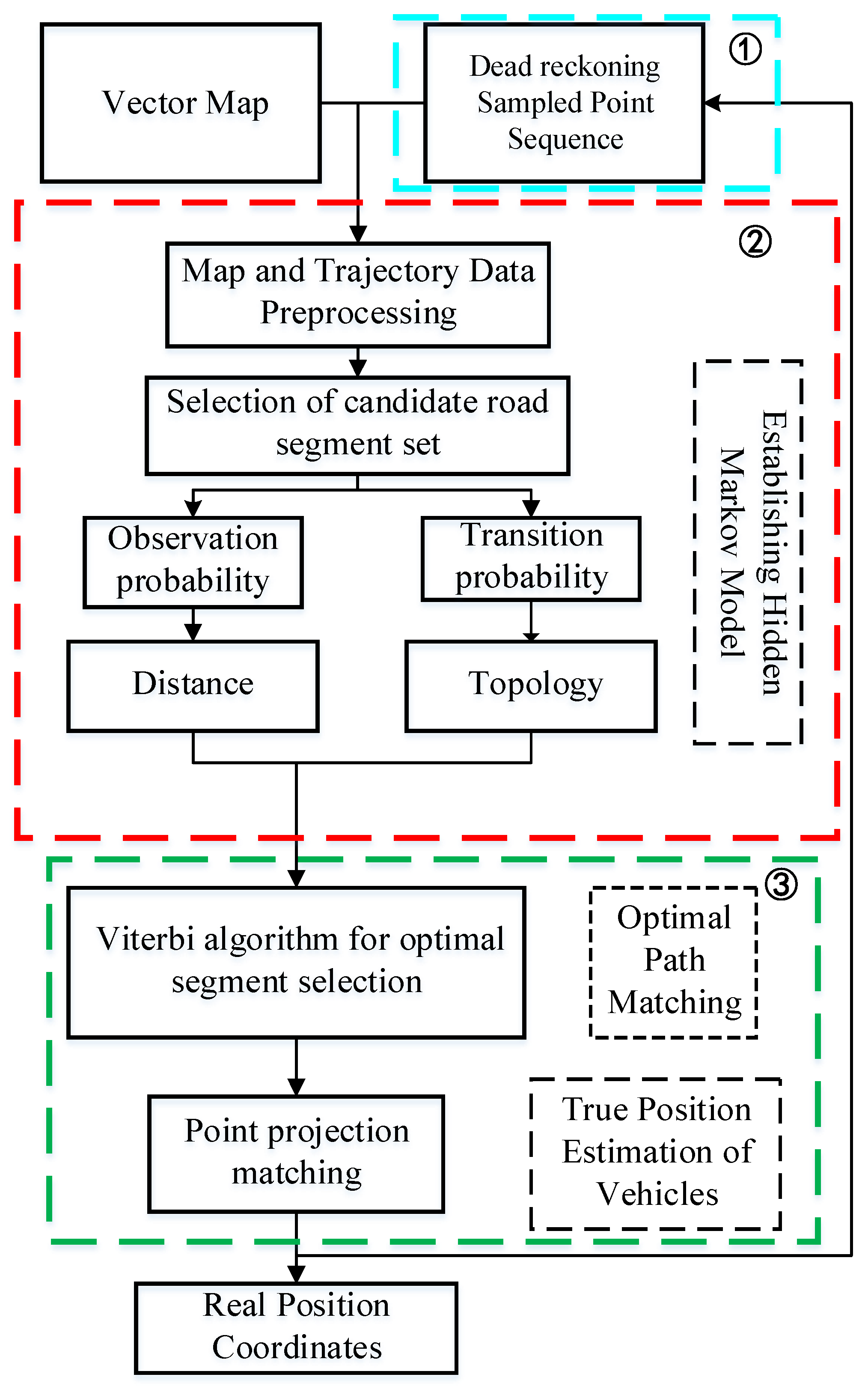
3. Overall Design of the Lane Level Positioning Method

Figure 1 shows the overall scheme of the proposed positioning method, which mainly contains three parts. Firstly, the sampled point sequence can be obtained by the inertial navigation system, which consists of optical fiber IMU and odometer. Secondly, the map matching model based on HMM is established, which contains data preprocessing and candidate segment selection. The input of this part is the vector map and the sampled point sequence. Its output are the candidate segments. Finally, the optimal path is solved based on Viterbi algorithm, and the positioning results are given.

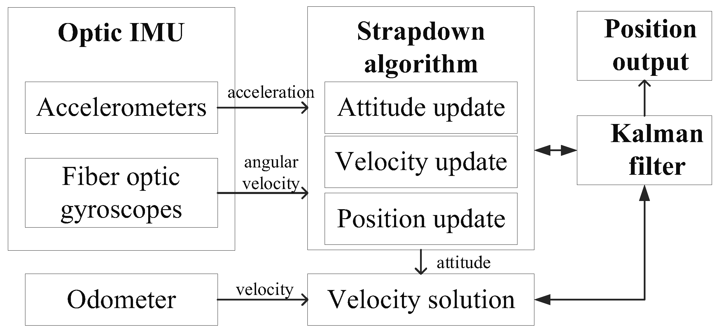
4. Dead Reckoning Principle Based on Optical Fiber IMU/Odometer

Dead reckoning is a process of estimating the vehicle’s trajectory and the coordinates of the current position relative to the initial position by using the navigation parameters such as the carrier’s attitude and speed, which are shown in Figure 2.
Taking n-frame as a reference, the attitude differential equation can be written as:
C ˙ b n = C b n ( ω n b b × )
where ω n b b denotes the angular rate under b-frame relative to n-frame, ( × ) represents the antisymmetric operation and ( ) means the differential operation. C b n represents the transformation matrix from b-frame to n-frame.
The output of the fiber optic gyroscope is the carrier’s angular rate under i-frame, which can be expressed as:
ω i b b = ω n b b + C n b ω i n n
where ω i b b means the carrier’s angular rate under i-frame, ω i n n is the angular rate under n-frame relative to i-frame and C n b = C b n T .
The odometer obtains the speed and displacement of the vehicle by measuring the wheel speed information during the vehicle driving process, taking the speed constraint into consideration; that is, there is speed only in the front direction. As a consequence, the speed of the vehicle can be written as:
v D b = 0 v D b 0 T = v D E b v D N b v D U b T
where v D b denotes the vehicle’s speed and the superscript b indicates that it is under b-frame. v D b refers to the forward speed measured by the odometer and v D U b is the vertical component. v D N b and v D E b are the east and the north component of the vehicle’s speed under b-frame, respectively.
Equation (4) can be obtained by converting v D b to n-frame:
v D n = C b n 0 v D b 0 = v D E n v D N n v D U n
where v D n is the output velocity output by the odometer under n-frame. v D E n , v D N n and v D U n are the east, the north and the vertical component of the vehicle’s speed under n-frame separately.
The differential equation of dead reckoning can be obtained according to the odometer’s output, which can be expressed as follows:
L ˙ D = v D N n R M h D λ ˙ D = v D E n sec L D R N h D h ˙ D = v D U n
Changing Equation (5) into vector form:
p ˙ D = M pvD v D n
where p D = L D λ D h D T , L D is the latitude calculated by dead reckoning, λ D is the longitude computed by dead reckoning and h D is the height determined by dead reckoning.
The following relationship comes into existence:
R M h D = R M D + h D R N h D = R N D + h D
where R M D and R N D are the radius of curvature in prime vertical in meridian circle and prime vertical separately. On the other hand, M p v D can be obtained by Equation (8):
M p v D = 0 1 / R M h D 0 sec L D / R N h D 0 0 0 0 1
In the attitude differential equation (Equation (1)), the speed of IMU is replaced by the speed output by the odometer, and the latitude estimated by IMU is replaced by that of dead reckoning. So, the attitude matrix differential equation of dead reckoning can be obtained as follows:
C ˙ b n = C b n ( ω i b b × ) ( ω i n n × ) C b n
Furthermore, Equation (10) also holds:
ω i n n = ω i e n + ω e n n ω i e n = 0 ω i e cos L D ω i e sin L D T ω e n n = v D N n R M h D v D E n R N h D v D E n tan L D R N h D T
where ω i e n is the angular rate caused by the Earth’s rotation under n-frame and ω e n n denotes the angular rate caused by the change of carrier’s speed. ω i e denotes the velocity of the earth’s rotation, which is usually taken as 15°/h.
In combination with Equations (3)–(10), the attitude and position update of the vehicle can be obtained.

5. Map Matching Model Based on HMM

HMM is often used in time series data modeling in various fields. Usually, the observation sequence and transition relationship are known to solve the hidden sequence, and the Viterbi algorithm is a typical solution algorithm. The model diagram applicable to the application scenario of this paper is shown in Figure 3.
As shown in Figure 3, the observation sequence and the hidden sequence correspond to the sampled point and the optimal road segments, respectively. The purpose of this paper is to set up a reasonable transfer relationship, so as to solve the optimal road segments. Different from the existing methods, we take the positioning error of the inertial system as a priori information to select the candidate road segments. The specific implementation of the model will be described in detail below.

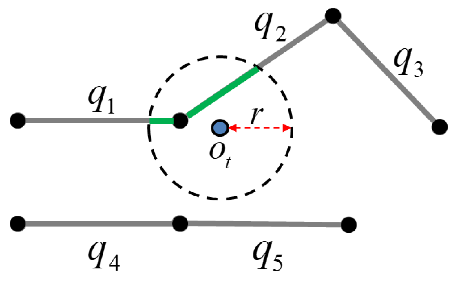
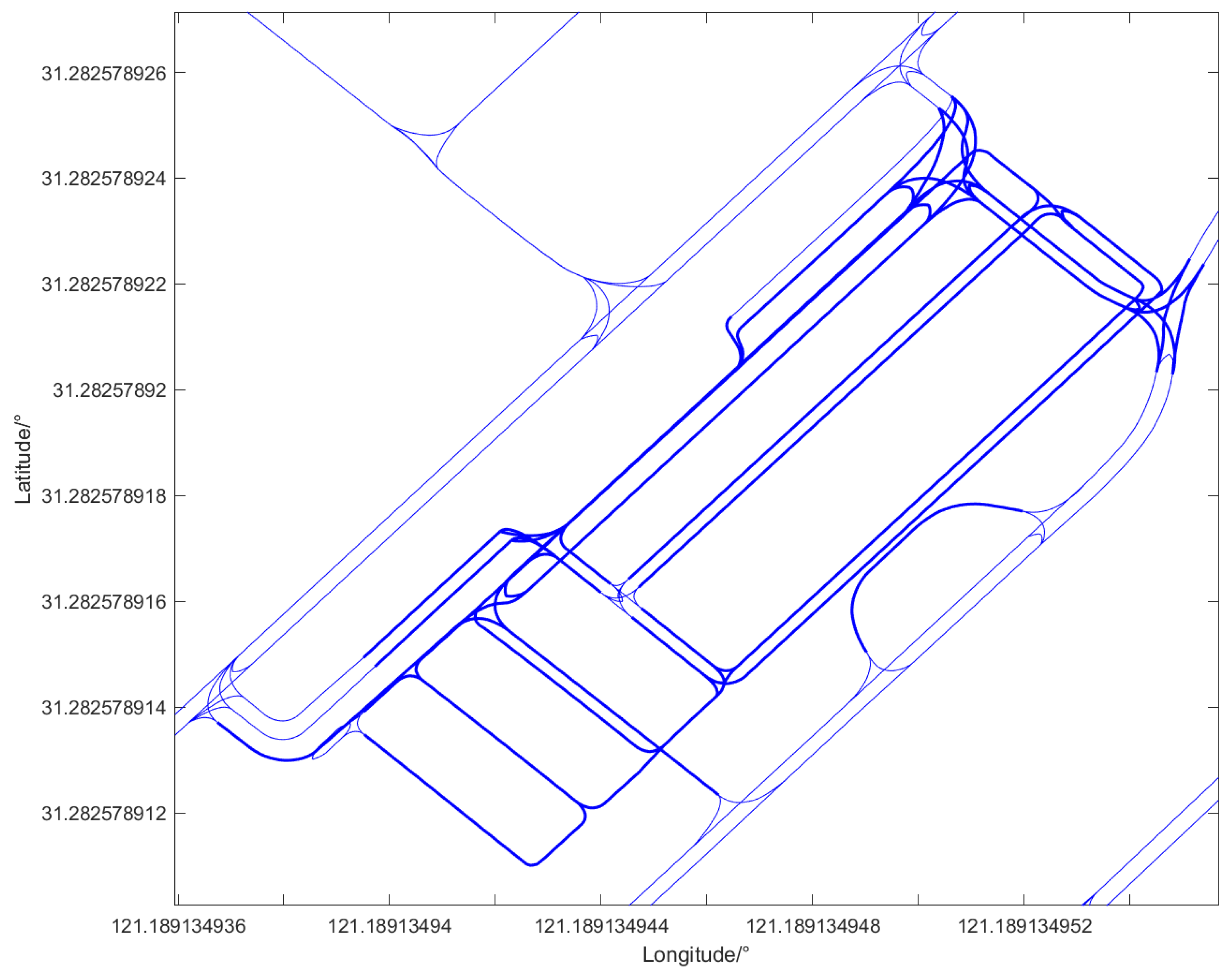
5.1. Selection of Candidate Road Segments

In order to limit the number of candidate road segments, only the road segments near the sampled points sequence are taken as the hidden state set. The candidate road segments set is obtained by establishing the positioning circle, which is shown in Figure 4.
Assuming that point o t is the sampled point of dead reckoning system at time t, we can obtain the positioning circle with point o t as the center and r as the radius. It can be seen from Figure 4 that segment q1 and q2 intersect with the positioning circle, so they are selected as candidate segments. Obviously, the value of the radius determines the number of candidate road segments. In order to be more reasonable, the radius of the positioning circle is designed according to the positioning error of the dead reckoning system.

5.2. Initial Distribution Probability

By designing the positioning circle, the candidate road segments that meet certain conditions are selected as the hidden state set in HMM. On the premise of knowing the set of hidden states Q , it is essential to compute the initial distribution probability to obtain the complete parameter of HMM. The initial distribution probability means the possibility of observing the first sampled point in each segment at the initial time, which can be expressed by the Euclidean distance to each candidate segment. Figure 5 explains its principle.
As shown in Figure 5, the road segment e 3 e 4 is equal to MN. o 1 , o 2 and o 3 are three sampled points obtained by the dead reckoning system. Their coordinates are x 1 , y 1 , x 2 , y 2 and x 3 , y 3 , respectively. M and N are the two endpoints of the road segment, whose coordinates are m 1 , n 1 and m 2 , n 2 separately. When calculating the Euclidean distance from the sampled point to the candidate road segment, it is mainly divided into two cases: the foot point of the dead reckoning sampled point is on the road segment or on the extension line on both sides of the road segment. When the point is o 1 in Figure 5, its foot point is P, which is on the line MN. Consequently, the Euclidean distance from o 1 to the candidate road segment is the length of h 1 , which can be computed by Equation (11):
h 1 = x 1 n 2 n 1 y 1 m 2 m 1 m 1 n 2 m 2 n 1 m 2 m 1 2 + n 2 n 1 2
When the projection of the sampled point is on the extension line of the candidate segment, for the reason that the extension line of the road segment has only mathematical meaning and no physical meaning, and does not exist in the actual vector map, the Euclidean distance between the positioning point and the foot point on the extension line of the line segment cannot be used as the distance between the sampled point and the candidate segment. At this time, the distance from the sampled point to the candidate segment is calculated according to the distance between the sampled point and the nodes at both ends of the candidate segment. Taking o 3 for example, it is obvious that its projection h 3 is smaller than h 2 . Therefore, the Euclidean distance between o 3 and the candidate segment is h 3 , which can be calculated by Equation (12):
h 3 = x 3 m 1 2 + y 3 n 1 2
After obtaining the distance information, the initial distribution probability function is defined as:
= 1 / h
where h is the Euclidean distance between the sampled point and the candidate segment.

5.3. Transition Probability

Transition probability describes the probability of transition from one state value to another at the current time. In our proposed method, transition probability p i t + 1 = q j i t = q i means the probability of transition from segment q i to q j . i t + 1 means the sampled point at time t + 1. The frequency of the sampled points sequence obtained by the dead reckoning system is 10 Hz, illustrating that the average distance between two adjacent sampled points is about 1.4 m~2.2 m. Furthermore, the average length of road segments in the vector map is generally more than 10 m. As a consequence, the correct matching segment corresponding to the sampled point at the current time is the same or directly connected with the matching segment at previous time. So, the transition probability of the situation that two adjacent sampled points belong to the same candidate segment can be calculated by Equation (14):
p ( i t + 1 i t ) = D m e a n d o t o t + 1 D m e a n
where D m e a n denotes the average length of the candidate segments set, d o t o t + 1 means the distance between two adjacent sampled points.
On the contrary, the transition probability of the situation that the two adjacent sampled points belong to two directly connected segments can be computed by Equation (15):
1 p ( i t + 1 i t ) = d o t o t + 1 D m e a n

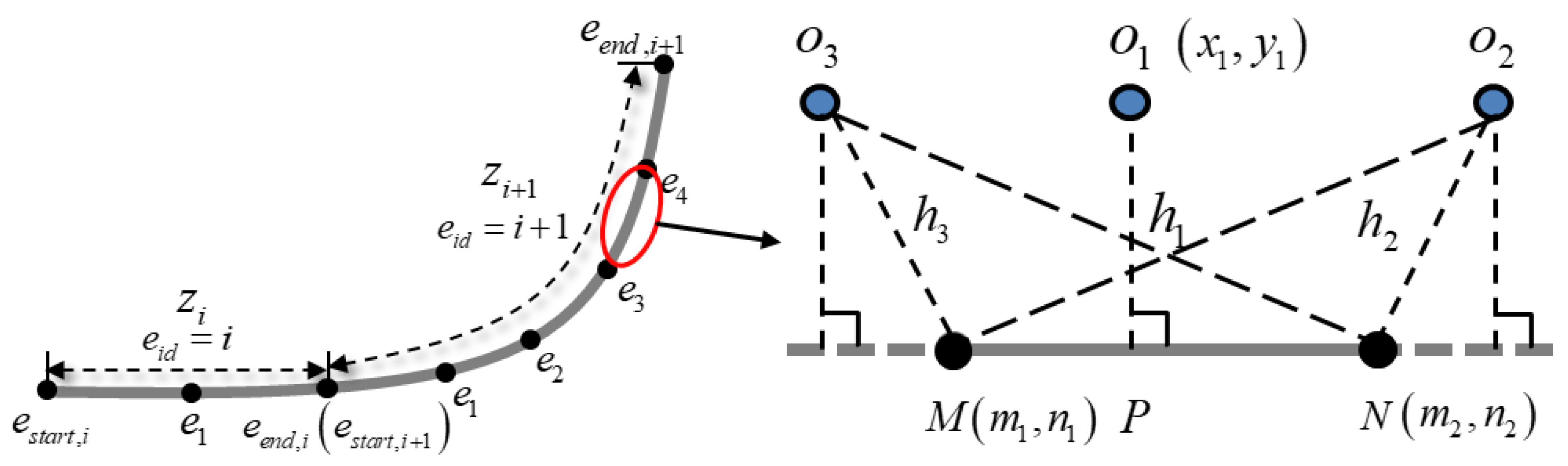
5.4. Observation Probability

The observation probability P o t | i t = q j is defined as the probability that the sampled point i t belongs to the candidate segment q j , which can be expressed as Equation (16):
p o t q j = 1 / d o t q j l = 1 N 1 / d o t q j
where N means the number of candidate segments, d o t q j represents the Euclidean distance between the sampled point i t and the candidate segment q j .

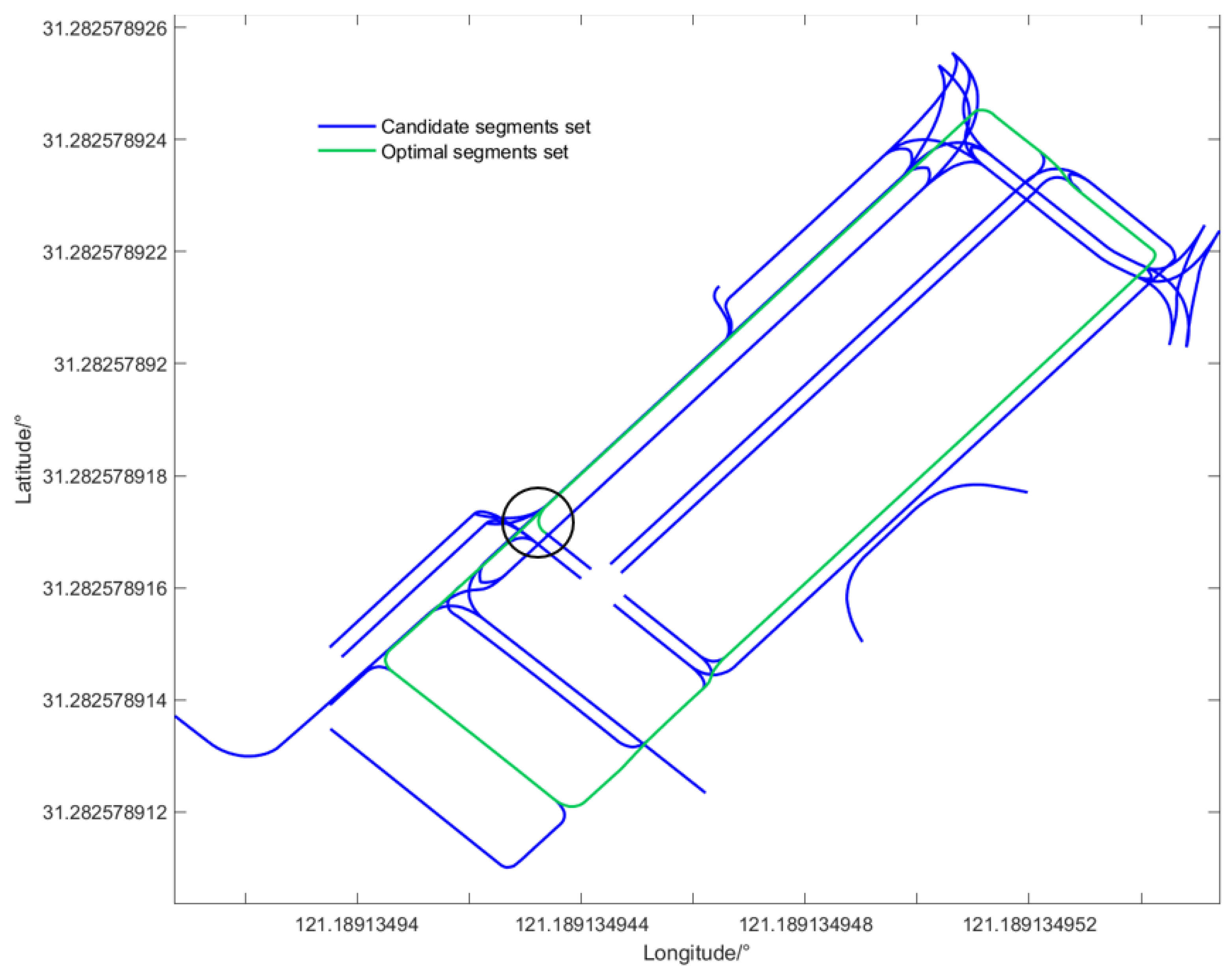
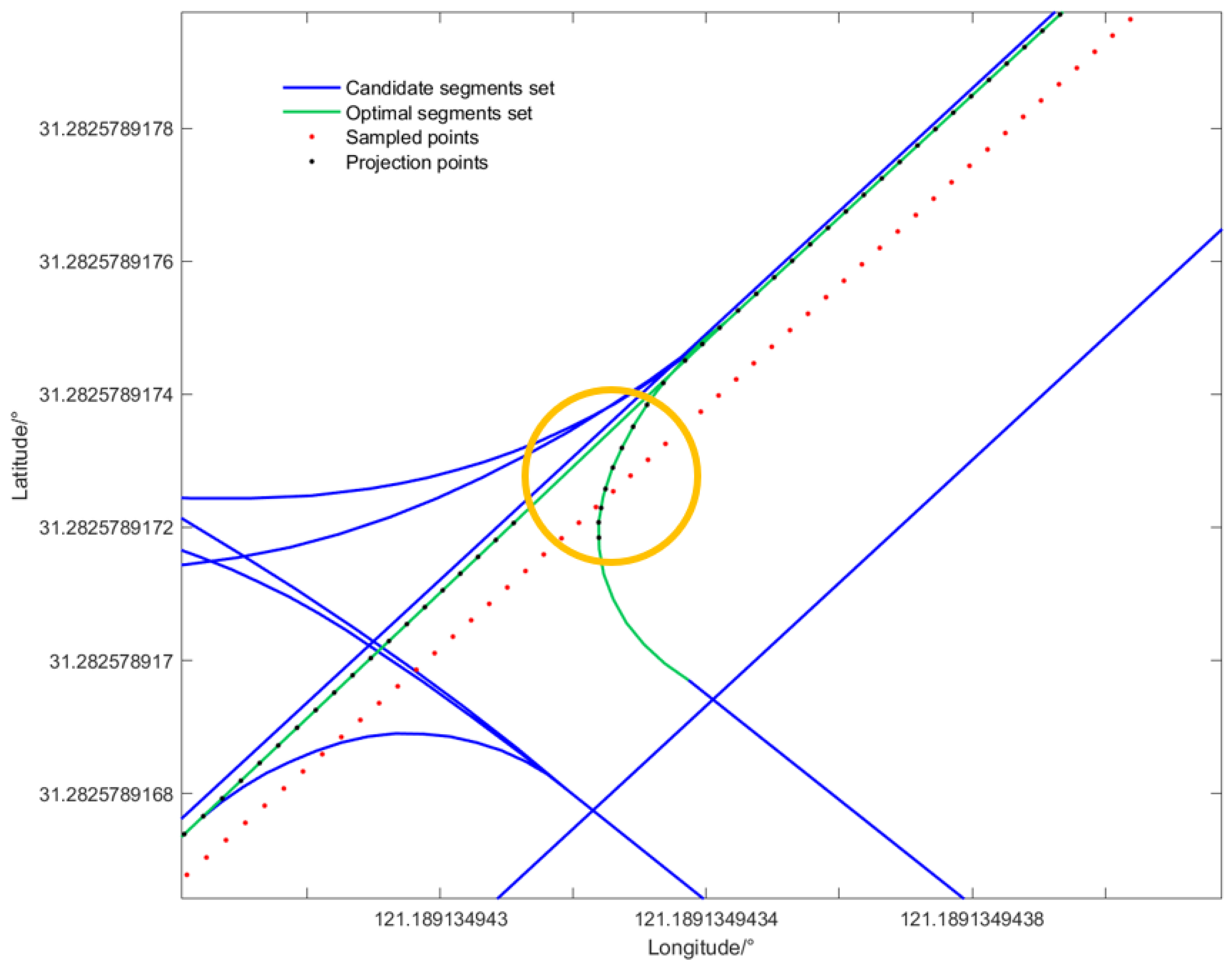
6. Optimal Path Selection Based on Viterbi Algorithm

The Viterbi algorithm recurses the state value probability at each time, and takes the last time as the termination condition to obtain the joint probability of the optimal path at the previous time, which can be described as Equation (17):
P j o int = Π P T P O
where P j o int is the logarithmic joint probability; P T and P O are transition probability and observation probability, respectively.
According to the known candidate road segment set Q = q 1 , q 2 , , q N and sampled point sequence obtained by dead reckoning system I = i 1 , i 2 , , i T , based on the Viterbi algorithm, through local state recursion and state backtracking, the real road segment that the vehicle has traveled can be obtained. Algorithm 1’s pseudo code is shown as below.
Algorithm 1: Viterbi Algorithm
Input: Collection of candidate road segments Q = q 1 , q 2 , , q N ,
Sampled points set I = i 1 , i 2 , , i T
Output: Optimal Segment Sequence Q = q 1 , q 2 , , q T
1:  Let P denote the highest score;
2:  Let Q [ ] denote the set of the optimal segments;
3:    t 1
4:  Set i
5:  for  j 1 to N  do
6:    P 1 = Π j
7:    q 1 = q j
8:   Q = Q + q 1 ;
9:  end for
10:  for  t 2 to T  do
11:    for  j 1 to N  do
12:     P j = P T j P O j
13:     q t = q j
14:    Q = Q + q t
15:    end for
16:  end for
17:  return Q = q 1 , q 2 , , q T
After the optimal matching road segments are obtained, the sampled point needs to be projected on the road segment to obtain the final positioning result. In this paper, the sampling frequency of the sampled point obtained by the dead reckoning system is 10 Hz, which belongs to high-frequency positioning data in the field of map matching. Therefore, the vertical projection method is finally used to project the sampled point to the optimal matching road segment. When the pedal is on the road segment, then it is the final estimated position corresponding to the sampled point. When the pedal is on the extension line of the road segment, then the end point of the road segment closest to the sampled point is the final estimation position.

7. Evaluation Method

Combined with the established model, three evaluation methods are used to evaluate the correctness of the model. Firstly, the driving route of the test vehicle has been planned in advance, so the real road segments that the test vehicle traveled are manually marked as the ground truth. In addition, they are matched with the optimal matching path identified by the Viterbi algorithm. For comparison, the correct rate of road segment matching is measured by defining the recall rate, which can be written as:
R e c a l l = T P T P + F P × 100 %
where T P is the number of the correctly identified road segments; F P is the number of the wrongly identified road segments on the contrary.
In order to measure the projection accuracy of the sampled point in the optimal matching road segment, the correct matching percentage (CMR) is defined as:
C M R =   N T   N T + N F × 100 %
where N T is the number of correctly matched points and N F is the number of wrongly matched points.
The positioning error of the whole method is defined as Equation (20):
P E =   S 1   N 3
where S 1 is the sum of the distance between the sampled pointed and the ground truth after or before matching, N 3 is the total number of sampled points.

8. Experiment and Discussion

Based on the above analysis, this section carries out the verification experiment. The verification experiments are implemented in the park of an automobile company in Beijing, and the vector map, which is shown in Figure 6, is also provided by the company. The specific forms of the vector map are high-precision longitude and latitude coordinate pairs, which are collected and calibrated by laser radar and a high-precision optical fiber inertial measurement unit. The accuracy of the vector map can reach the centimeter level. The segments concluded in the red box in Figure 6, shown in Figure 7, are the underground garage, where the proposed positioning scheme is verified.
The vehicle used in the experiment and the detailed device configuration are shown in Figure 8 and Figure 9, respectively. The specific parameters of the optical fiber IMU used in the validation experiments are listed in Table 3. The odometer used in the experiment is provided by the vehicle itself.
In addition, the test vehicle is equipped with a high-precision inertial navigation system whose output trajectory is regarded as the ground truth to measure the error of the proposed method. Its gyroscope and accelerometer bias are 0.01°/h and 50 ug, respectively.
A total of two validation experiments have been carried out, and the specific conditions are described as follows:
Case 1: 
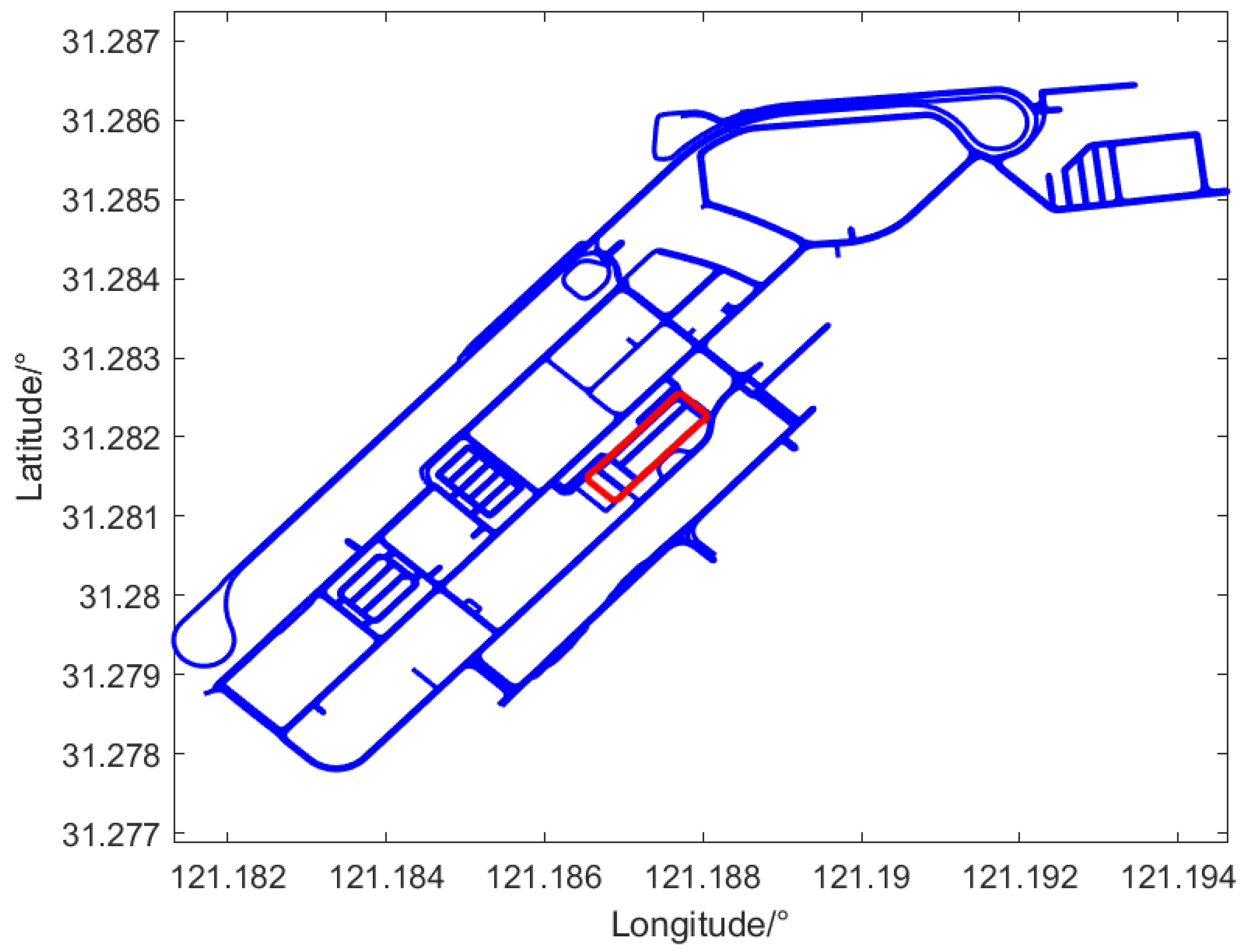
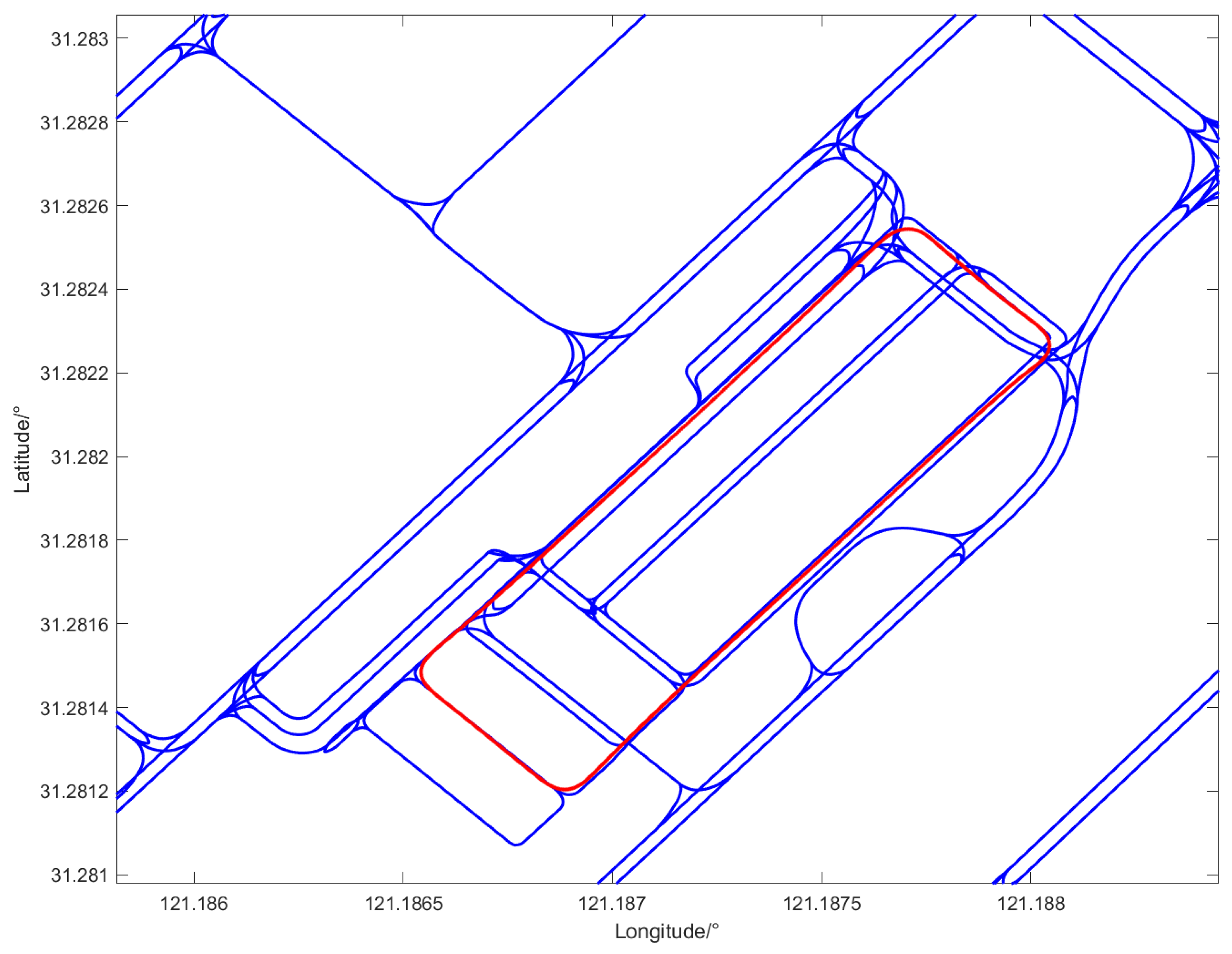
The vehicle starts from the northeast corner of the map and drives along the lane line to the southwest corner of the map. The vehicle drives eight laps in the underground garage. The red line in Figure 10 represents the track of the vehicle. A curve is selected in the lower right corner of Figure 10 and enlarged locally for better visualization.
Case 2: 
The vehicle drives one lap in the underground garage. There are more curves and more complicated road conditions.
In both cases, the vehicle’s speed is about 30 km/h.
The initial positions of the two cases are the positions when the satellite signal is missing, which can be judged according to the flag of the data. The trajectories obtained by the inertial system of the second and eighth lap in case 1 are selected for verification. Similarly, the trajectory in case 2 is also selected for verification. For convenience, we define that S1 and S2 denote the trajectories obtained by the inertial system of the second and eighth lap in case 1, respectively. S3 represents the trajectory in case 2. The frequency of the trajectory obtained by the inertial system in this paper is 10 Hz.
Based on the characteristics of inertial system error accumulation over time, the radius of the positioning circle of S1, S2 and S3 is set to 5 m, 10 m and 5 m, respectively. The candidate road segment set is obtained according to the inertial trajectory, positioning circle and vector map. Among them, the set of candidate segments corresponding to S2 are shown in Figure 11. The number of sampled points, actual driving distance, inertial calculation distance, positioning circle radius and the number of candidate segments corresponding to the three trajectories are summarized in Table 4.
It can be seen from Table 4 that the radius of the positioning circle directly affects the number of candidate segments and indirectly affects the execution time of the algorithm. Obviously, the sampled points corresponding to trajectory S2 are the least, but the candidate segments are the most for the reason that the radius is the largest. Furthermore, the number of sampled points of trajectory S3 is obviously more than S1, but there is little difference between the candidate segments, illustrating that one candidate road segment contains many sampled points. It also proves the rationality of the principle of transition probability.
After obtaining the candidate segments set, it is necessary to further calculate the initial distribution probability, transition probability and observation probability, so as to obtain the optimal matching segments set. The initial distribution probability and observation probability are calculated based on the Euclidean distance from the sampled point to the candidate road segment, which has been described in Section 5. The parameters required to calculate the transition probability are summarized in Table 5. As can be seen from Table 5, the distance between adjacent sampled points corresponding to trajectory S2 is greater than trajectory S1 and S3. The potential reason may be that the error of trajectory S2 is relatively large, because the test vehicle has been driving for a long time in the underground garage.
The Viterbi algorithm is used to optimize the path of the candidate segments set of three experiments, and the optimal matching segments set is obtained. Among them, the optimal matching segments corresponding to trajectory S2 is shown in Figure 12. Finally, the final location results can be obtained by projecting the sampled points onto the optimal candidate road segments.
In the process of optimal segment matching, there will be mismatching. The black circle in Figure 12 represents a typical example. The place represented by the black circle is a trigeminal intersection, which is composed of two segments into one segment. Figure 13 shows the specific situation of the black circle. As can be seen in Figure 13, the red points denote the sampled points; on the other hand, the black points represent the projection points. It can be seen from the trajectory of the red points that the test vehicle is driven in a straight line. However, the result of our algorithm is from straight line to curve, which is definitely unreasonable. In more detail, when approaching the curve, the sampled points are closer to the curved segment than the straight segment, which directly causes the wrong matching result.
In general, the current model depends on the distance to select the road segments, which has limitations. As a consequence, the wrong matching result specifically provides ideas for the improvement of the model. For instance, if the direction information of the test vehicle were taken into consideration, the situation shown in Figure 13 would not occur.
According to the evaluation method proposed in Section 7, the results of the three experiments are summarized in Table 6. Based on the gyroscope and accelerometer in Table 3 and the odometer provided by the vehicle, we can obtain the driving trajectory of the carrier. Comparing this trajectory with the ground truth, we can compute the positioning error of the inertial system, which is the ‘PE before matching’ in Table 6. Obviously, without map matching, the positioning errors of three experiments are 0.59 m, 1.03 m and 0.84 m, respectively. Then, we use the proposed integrated positioning method to estimate the vehicle’s driving trajectory, which is compared with the ground truth. As a consequence, the corresponding positioning error of the proposed method can be obtained, which is the ‘PE after matching’ in Table 6. It is not difficult to see that the positioning errors of the proposed integrated positioning methods corresponding to trajectory S1, S2 and S3 are 0.12 m, 0.24 m and 0.18 m, respectively.
Compared to inertial system, the positioning error is greatly reduced, demonstrating the effectiveness of the proposed method. In addition, the proposed method is not affected by the environment. As long as the vector maps are collected in advance, they can be reused, facilitating large-scale promotion and application in GNSS denied environments such as underground parking lots and large logistics complex areas.
Furthermore, it can be seen that the recall corresponding to trajectory S1 and S3 is 100%, which represents that all the optimal road segments are the actual driving segments of the test vehicle. Actually, the inertial positioning errors of these two trajectories are small because the test vehicle does not travel for a long time. The positioning errors after matching have been reduced to lower than 20 cm, which also exactly proves the superior performance of the proposed method when the inertial error is small. For trajectory S3, more complex road conditions directly lead to lower accuracy. On the other hand, the inertial error of trajectory S2 is large, so the recall is 94.4%, which is smaller than others.
The experimental results show that the proposed method can achieve lane level positioning accuracy under the GNSS denied environments. In terms of running time, the number of sampled points play a decisive role, which also brings a new problem. If there is a need for real-time performance, the proposed algorithm still needs to be further optimized.

9. Conclusions

At present, most map matching algorithms take GNSS trajectory as a priori information to estimate the real driving trajectory of vehicles, which is not applicable under GNSS denied environments. However, the error of inertial system will accumulate over time and it cannot provide good performance for a long time. Aiming at the demand of unmanned driving for high-precision positioning, this paper puts forward a lane level positioning method based on inertial system and vector map information fusion. The trajectory obtained from dead reckoning and vector map are regarded as priori information; lane level positioning results are obtained based on the established map matching model. Experimental results show that the positioning error of the proposed method is less than 30 cm when driving for about 7 min, which meets the application requirements of unmanned driving. However, the proposed method can be optimized by adding heading information to avoid false matches and improving real-time performance. Moreover, further optimization and evaluation of the proposed method through longer distance and more reasonable probability function will be carried out in the next work.

Author Contributions

Conceptualization, M.D. and H.L.; methodology, M.D. and J.L.; software, Y.T.; validation, M.D., J.C. and Y.W.; formal analysis, M.D.; investigation, Y.W.; resources, H.L.; data curation, M.D. and H.L.; writing—original draft preparation, M.D.; writing—review and editing, H.L.; visualization, X.P.; supervision, C.Z.; project administration, C.Z. All authors have read and agreed to the published version of the manuscript.

Funding

This research received no external funding.

Data Availability Statement

All data and models used during the study appear in the submitted article.

Conflicts of Interest

The authors declare that they have no known competing financial interest or personal relationship that could have appeared to influence the work reported in this paper.

References

  1. Guo, J.; Kurup, U.; Shah, M. Is It Safe to Drive? An Overview of Factors, Metrics, and Datasets for Driveability Assessment in Autonomous Driving. IEEE Trans. Intell. Transp. Syst. 2020, 21, 3135–3151. [Google Scholar] [CrossRef]
  2. Liu, W.; Li, Z.; Sun, S.; Gupta, M.K.; Du, H.; Malekian, R.; Sotelo, M.A.; Li, W. Design a Novel Target to Improve Positioning Accuracy of Autonomous Vehicular Navigation System in GPS Denied Environments. IEEE Trans. Ind. Inform. 2021, 17, 7575–7588. [Google Scholar] [CrossRef]
  3. Ye, L.; Gao, N.; Yang, Y.; Li, X. A High-Precision and Low-Cost Broadband LEO 3-Satellite Alternate Switching Ranging/INS Integrated Navigation and Positioning Algorithm. Drones 2022, 6, 241. [Google Scholar] [CrossRef]
  4. Syed, Z.F.; Aggarwal, P.; Niu, X.; El-Sheimy, N. Civilian Vehicle Navigation: Required Alignment of the Inertial Sensors for Acceps Navigation Accuracies. IEEE Trans. Veh. Technol. 2008, 57, 3402–3412. [Google Scholar]
  5. Zhang, Z.; Niu, X.; Tang, H.; Chen, Q.; Zhang, T. GNSS/INS/ODO/Wheel Angle Integrated Navigation Algorithm for an All-Wheel Steering Robot. Meas. Sci. Technol. 2021, 32, 115122. [Google Scholar] [CrossRef]
  6. Gu, N.; Xing, F.; You, Z. Visual/Inertial/GNSS Integrated Navigation System under GNSS Spoofing Attack. Remote Sens. 2022, 14, 5975. [Google Scholar] [CrossRef]
  7. Zhao, H.; Miao, L.; Shao, H. Adaptive Two-Stage Kalman Filter for SINS/Odometer Integrated Navigation Systems. J. Navig. 2017, 70, 242–261. [Google Scholar] [CrossRef] [Green Version]
  8. Bai, H.; Xue, X. Simulation Research on FOG-SINS/Doppler Radar/Baro-Altimeter Integrated Navigation for Helicopters. In Proceedings of the 2010 Second International Conference on Computer Modeling and Simulation, Sanya, China, 22–24 January 2010; pp. 115–119. [Google Scholar]
  9. Shan, B.; Qin, Y.; Wang, Y.; Yang, B.; Guo, Z. SINS/Geomagnetic Matching/Barometric Altimeter Integrated Navigation Method for Land Vehicle. In Proceedings of the 2014 IEEE International Conference on Signal Processing, Communications and Computing (ICSPCC), Guilin, China, 5–8 August 2014; pp. 32–35. [Google Scholar]
  10. Ren, Y.; Wang, L.; Lin, K.; Ma, H.; Ma, M. Improved Iterative Closest Contour Point Matching Navigation Algorithm Based on Geomagnetic Vector. Electronics 2022, 11, 796. [Google Scholar] [CrossRef]
  11. Shahoud, A.; Shashev, D.; Shidlovskiy, S. Visual Navigation and Path Tracking Using Street Geometry Information for Image Alignment and Servoing. Drones 2022, 6, 107. [Google Scholar] [CrossRef]
  12. Duo, J.; Zhao, L. A Robust and Efficient Airborne Scene Matching Algorithm for UAV Navigation. In Proceedings of the 2017 IEEE 9th International Conference on Communication Software and Networks (ICCSN), Guangzhou, China, 6–8 May 2017; pp. 1337–1342. [Google Scholar]
  13. Zhang, T.; Liu, C.; Li, J.; Pang, M.; Wang, M. A New Visual Inertial Simultaneous Localization and Mapping (SLAM) Algorithm Based on Point and Line Features. Drones 2022, 6, 23. [Google Scholar]
  14. Zhai, C.; Wang, M.; Yang, Y.; Shen, K. Robust Vision-Aided Inertial Navigation System for Protection Against Ego-Motion Uncertainty of Unmanned Ground Vehicle. IEEE Trans. Ind. Electron. 2021, 68, 12462–12471. [Google Scholar] [CrossRef]
  15. Liu, X.; Sun, X.; Xia, X. LiDAR Point’s Elliptical Error Model and Laser Positioning for Autonomous Vehicles. Meas. Sci. Technol. 2020, 32, 035107. [Google Scholar] [CrossRef]
  16. Du, B.; Shi, Z.; Wang, H.; Han, L.; Song, J. Multi-Layer Model Aided Inertial Navigation System for Unmanned Ground Vehicles. Meas. Sci. Technol. 2022, 33, 075110. [Google Scholar] [CrossRef]
  17. Chen, W.; Li, X.; Song, X.; Li, B.; Song, X.; Xu, Q. A Novel Fusion Methodology to Bridge GPS Outages for Land Vehicle Positioning. Meas. Sci. Technol. 2015, 26, 075001. [Google Scholar] [CrossRef]
  18. Aggarwal, P.; Thomas, D.; Ojeda, L.; Borenstein, J. Map Matching and Heuristic Elimination of Gyro Drift for Personal Navigation Systems in GPS-Denied Conditions. Meas. Sci. Technol. 2011, 22, 025205. [Google Scholar] [CrossRef] [Green Version]
  19. Zhang, J.; Khodabandeh, A.; Khoshelham, K. Centimeter-Level Positioning by Instantaneous Lidar-Aided GNSS Ambiguity Resolution. Meas. Sci. Technol. 2022, 22, 115020. [Google Scholar] [CrossRef]
  20. Arafat, M.Y.; Alam, M.M.; Moh, S. Vision-Based Navigation Techniques for Unmanned Aerial Vehicles: Review and Challenges. Drones 2023, 7, 89. [Google Scholar] [CrossRef]
  21. Antonopoulos, A.; Lagoudakis, M.G.; Partsinevelos, P. A ROS Multi-Tier UAV Localization Module Based on GNSS, Inertial and Visual-Depth Data. Drones 2022, 6, 135. [Google Scholar] [CrossRef]
  22. Ling, Y.; Chu, X.; Lu, Z.; Wang, L.; Wen, X. PCM: A Positioning Calibration Mechanism for Connected Autonomous Vehicles. IEEE Access 2020, 8, 95046–95056. [Google Scholar] [CrossRef]
  23. Lei, T.; Xiao, G.; Yin, X. Targeting Lane-Level Map Matching for Smart Vehicles: Construction of High-Definition Road Maps Based on GIS. Appl. Sci. 2023, 13, 862. [Google Scholar] [CrossRef]
  24. Kassas, Z.Z.M.; Maaref, M.; Morales, J.J.; Khalife, J.J.; Shamei, K. Robust Vehicular Localization and Map Matching in Urban Environments Through IMU, GNSS, and Cellular Signals. IEEE Intell. Transp. Syst. Mag. 2020, 12, 36–52. [Google Scholar] [CrossRef]
  25. Feng, J.; Li, Y.; Zhao, K.; Xu, Z.; Xia, T.; Zhang, J.; Jin, D. DeepMM: Deep Learning Based Map Matching with Data Augmentation. IEEE Trans. Mob. Comput. 2020, 21, 2372–2384. [Google Scholar] [CrossRef]
  26. Bernstein, D.; Kornhauser, A. An Introduction to Map Matching for Personal Navigation Assistants; Geometric Distributions; Tech. Rep.; New Jersey Institute of Technology: Newark, NJ, USA, 1998. [Google Scholar]
  27. White, C.E.; Bernstein, D.; Kornhauser, A.L. Some Map Matching Algorithms for Personal Navigation Assistants. Transp. Res. Part C Emerg. Technol. 2000, 8, 91–108. [Google Scholar]
  28. Taylor, G.; Blewitt, G.; Steup, D.; Corbett, S.; Car, A. Road Reduction Filtering for GPS-GIS Navigation. Trans. GIS 2001, 5, 193–207. [Google Scholar] [CrossRef]
  29. Zeng, Z.; Zhang, T.; Li, Q.; Wu, Z.; Zou, H.; Gao, C. Curvedness Feature Constrained Map Matching for Low-Frequency Probe Vehicle Data. Int. J. Geogr. Inf. Sci. 2016, 30, 660–690. [Google Scholar] [CrossRef]
  30. Sharma, K.P.; Jain, R. Inscribe the Exigency of Map Matching Performance for Curve Navigation on Road/Highways. In Proceedings of the 2019 Amity International Conference on Artificial Intelligence (AICAI), Dubai, United Arab Emirates, 4–6 February 2019; pp. 850–854. [Google Scholar]
  31. Fréchet, M.M. Sur Quelques Points Du Calcul Fonctionnel. Rend. Circ. Mat. Palermo 1906, 22, 1–72. [Google Scholar] [CrossRef] [Green Version]
  32. Bierlaire, M.; Chen, J.; Newman, J. A Probabilistic Map Matching Method for Smartphone GPS Data. Transp. Res. Part C Emerg. Technol. 2013, 26, 78–98. [Google Scholar] [CrossRef]
  33. Pink, O.; Hummel, B. A Statistical Approach to Map Matching Using Road Network Geometry, Topology and Vehicular Motion Constraints. In Proceedings of the 2008 11th International IEEE Conference on Intelligent Transportation Systems, Beijing, China, 12–15 October 2008; pp. 862–867. [Google Scholar]
  34. Ochieng, W.; Quddus, M.; Noland, R. Map-Matching in Complex Urban Road Networks. Braz. J. Cartogr. 2003, 55, 1–14. [Google Scholar] [CrossRef]
  35. Yue, Y.; Zhao, C.; Wen, M.; Wu, Z.; Wang, D. Collaborative Semantic Perception and Relative Localization Based on Map Matching. In Proceedings of the IEEE/RSJ International Conference on Intelligent Robots and Systems (IROS), Las Vegas, NV, USA, 24 October 2020–24 January 2021; pp. 6188–6193. [Google Scholar]
  36. Quddus, M.A.; Ochieng, W.Y.; Zhao, L.; Noland, R.B. A General Map Matching Algorithm for Transport Telematics Applications. GPS Solut. 2003, 7, 157–167. [Google Scholar] [CrossRef] [Green Version]
  37. Velaga, N.R.; Quddus, M.A.; Bristow, A.L. Developing an Enhanced Weight-Based Topological Map-Matching Algorithm for Intelligent Transport Systems. Transp. Res. Part C Emerg. Technol. 2009, 17, 672–683. [Google Scholar] [CrossRef] [Green Version]
  38. Yang, H.; Cheng, S.; Jiang, H.; An, S. An Enhanced Weight-Based Topological Map Matching Algorithm for Intricate Urban Road Network. Procedia Soc. Behav. Sci. 2013, 96, 1670–1678. [Google Scholar] [CrossRef] [Green Version]
  39. He, M.; Zheng, L.; Cao, W.; Huang, J.; Liu, X.; Liu, W. An Enhanced Weight-Based Real-Time Map Matching Algorithm for Complex Urban Networks. Phys. A Stat. Mech. Its Appl. 2019, 534, 122318. [Google Scholar] [CrossRef]
  40. Sharath, M.N.; Velaga, N.R.; Quddus, M.A. A Dynamic Two-Dimensional (D2D) Weight-Based Map-Matching Algorithm. Transp. Res. Part C Emerg. Technol. 2019, 98, 409–432. [Google Scholar] [CrossRef]
  41. Newson, P.; Krumm, J. Hidden Markov Map Matching through Noise and Sparseness. In Proceedings of the 17th ACM SIGSPATIAL International Conference on Advances in Geographic Information Systems, Seattle, WA, USA, 4–6 November 2009; pp. 336–343. [Google Scholar]
  42. Lou, Y.; Zhang, C.; Zheng, Y.; Xie, X.; Wang, W.; Huang, Y. Map-Matching for Low-Sampling-Rate GPS Trajectories. In Proceedings of the 17th ACM SIGSPATIAL International Conference on Advances in Geographic Information Systems, Seattle, WA, USA, 4–6 November 2009; pp. 352–361. [Google Scholar]
  43. Hsueh, Y.-L.; Chen, H.-C. Map Matching for Low-Sampling-Rate GPS Trajectories by Exploring Real-Time Moving Directions. Inf. Sci. 2018, 433–434, 55–69. [Google Scholar] [CrossRef]
  44. Hsueh, Y.-L.; Chen, H.-C.; Huang, W. A Hidden Markov Model-Based Map-Matching Approach for Low-Sampling-Rate GPS Trajectories. In Proceedings of the 2017 IEEE 7th International Symposium on Cloud and Service Computing (SC2), Kanazawa, Japan, 22–25 November 2017; pp. 271–274. [Google Scholar]
  45. Xie, Y.; Zhou, K.; Miao, F.; Zhang, Q. High-Accuracy Off-Line Map-Matching of Trajectory Network Division Based on Weight Adaptation HMM. IEEE Access 2020, 8, 7256–7266. [Google Scholar] [CrossRef]
  46. Sadli, R.; Afkir, M.; Hadid, A.; Rivenq, A.; Taleb-Ahmed, A. Map-Matching-Based Localization Using Camera and Low-Cost GPS for Lane-Level Accuracy. Sensors 2022, 22, 2434. [Google Scholar] [CrossRef] [PubMed]
Figure 1. The overall framework of the proposed lane level positioning method.
Drones 07 00239 g001
Figure 2. The principle of dead reckoning.
Drones 07 00239 g002
Figure 3. Hidden sequence solving model.
Drones 07 00239 g003
Figure 4. The schematic diagram of the positioning circle.
Drones 07 00239 g004
Figure 5. The schematic diagram of initial probability calculation.
Drones 07 00239 g005
Figure 6. The whole vector map and its road network structure.
Drones 07 00239 g006
Figure 7. The detailed structure of the red box in Figure 6.
Drones 07 00239 g007
Figure 8. The test vehicle.
Drones 07 00239 g008
Figure 9. The detailed experimental setup. ①: Fiber optic IMU, ②: Power supply, ③: Data transfer unit, ④: CAN module, ⑤: MOXA module, ⑥: Acquisition computer.
Drones 07 00239 g009
Figure 10. Trajectories of the test vehicle obtained by dead reckoning in case 1.
Drones 07 00239 g010
Figure 11. The set of candidate segments corresponding to trajectory S2.
Drones 07 00239 g011
Figure 12. The set of optimal segments corresponding to trajectory S2.
Drones 07 00239 g012
Figure 13. A typical mismatching example of trajectory S2.
Drones 07 00239 g013
Table 1. Several representative integrated positioning methods applicable to GNSS denied environments.
MethodTypical WorkAdvantageDisadvantage
SINS/OD[7]1. High autonomy;
2. Low cost;
1. Error accumulation exists;
SINS/Altimeter[8]1. Able to suppress divergence of altitude channel;
2. Low cost;
1. Low accuracy;
SINS/GMNS[9,10]1. No accumulated error;
2. Work all-weather;
1. Vulnerable to interference;
2. Low reliability;
SINS + SMNS[11,12]1. Low cost;
2. No accumulated error.
1. Difficulty in database collection;
2. Vulnerable to weather.
Table 2. Comparison of several representative map matching algorithms.
Specific
Algorithm
Typical
Work
TypeInformation
Source
Positioning
Accuracy
Line to line[24]Geometry-basedGPS5.5 m (80%)
Enhanced probability statistics[29]Probability statistics-basedGPS—— (85%)
Weighted topology matching[33]Road topology-basedGPS2.82 m (84%)
HMM[38]Integrated map matchingGPS1.3 m (98%)
Table 3. The specific parameters of the optical fiber IMU used in the validation experiments.
DeviceParameterValue
Fiber optic
gyroscope
Range±400°/s
Bias stability≤0.1°/h (1 σ )
Bias repeatability≤0.1°/h (1 σ )
Random walk coefficient≤0.02°/√h
Scale factor nonlinearity≤100 ppm
Scale factor repeatability≤100 ppm
Bandwidth≥200 Hz
AccelerometerRange±20 g
Bias stability≤0.2 mg (1 σ )
Bias repeatability≤0.2 mg (1 σ )
Random walk coefficient≤100 ppm
Scale factor nonlinearity≤100 ppm
Scale factor repeatability≥200 Hz
Table 4. Some parameters of three experiments.
TrajectoryNumber of
Sampled Points
Real Driving Distance (m)The Radius of the
Positioning Circle (m)
Number of
Candidate Segments
S11457420567
S213684201078
S32230550571
Table 5. The parameters required to calculate the transition probability.
TrajectoryAverage Length of Candidate Segments (m)Average Distance between Adjacent Sampled Points (cm)
S127.030.8
S230.249.8
S327.726.3
Table 6. Comparison of positioning accuracy of three test experiments.
TrajectoryRecallCMPPE before Matching (m)PE after Matching (m)Time of
Running (s)
S1100%100%0.590.1229.38
S294.4%98.57%1.030.2420.18
S3100%99.1%0.840.1847.43
Disclaimer/Publisher’s Note: The statements, opinions and data contained in all publications are solely those of the individual author(s) and contributor(s) and not of MDPI and/or the editor(s). MDPI and/or the editor(s) disclaim responsibility for any injury to people or property resulting from any ideas, methods, instructions or products referred to in the content.

