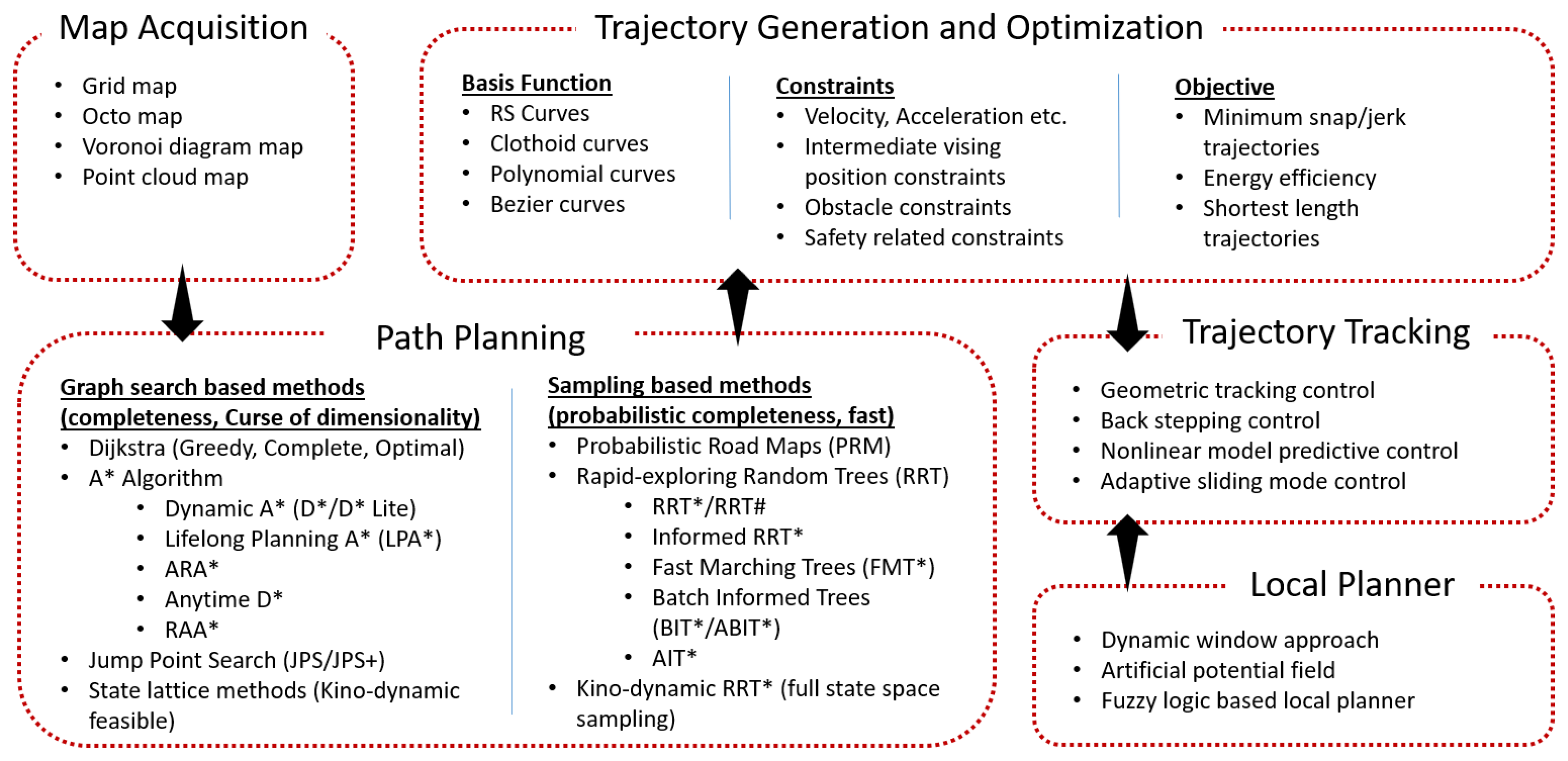
Figure 1.
Motion planning framework for mobile robots. Symbols (*, #) are part of the name of the method. RRT-Star (RRT*) is an improved version of RRT.
Figure 1.
Motion planning framework for mobile robots. Symbols (*, #) are part of the name of the method. RRT-Star (RRT*) is an improved version of RRT.
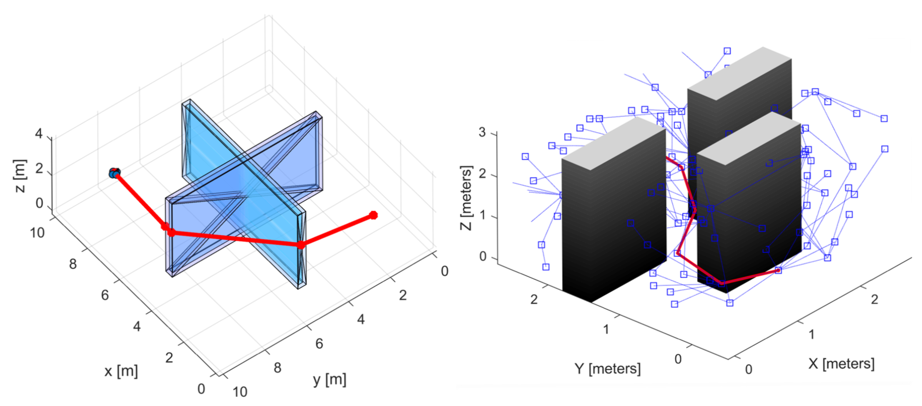
Figure 2.
Robotic path planning with the GBSA (JPS-3D) algorithm on the left and the SBS (RRT*) algorithm on right. The planned path through the environment is comprised of piece-wise line segments shown in red. Note the considerably small length of one segment in the path planned with the JPS-3D algorithm in close proximity to the thin wall.
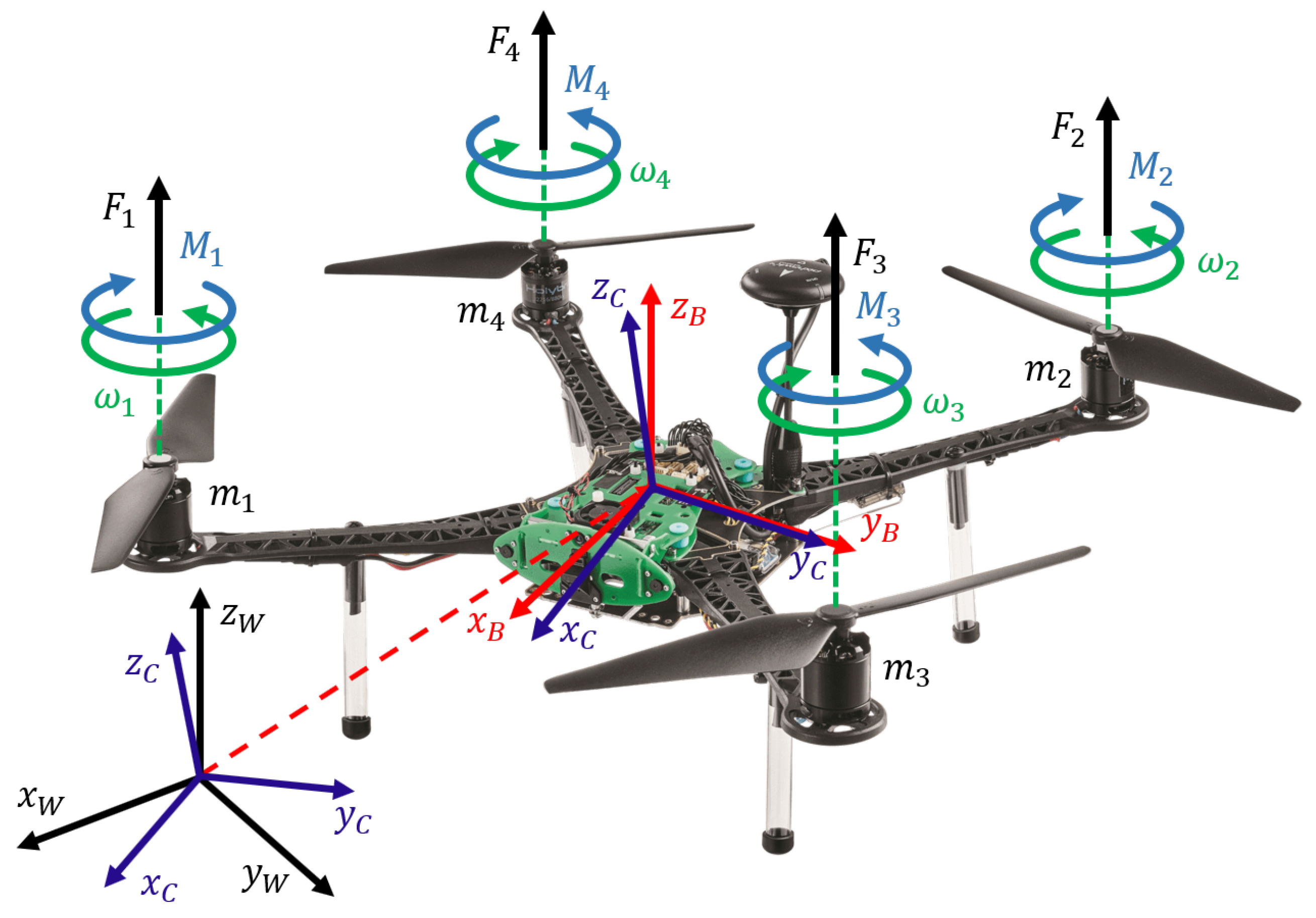
Figure 3.
Development drone (Manufactured by ModelAI, San Diego, CA, USA) with our Coordinate system. We consider three frames of reference namely World Frame, W (shown in black), Body Frame, B (shown in red), and a Camera Frame, C (shown in blue), with relevant axes . Forces, , moments, , and angular velocities, , produced by rotors are shown with black, blue, and green arrows respectively.
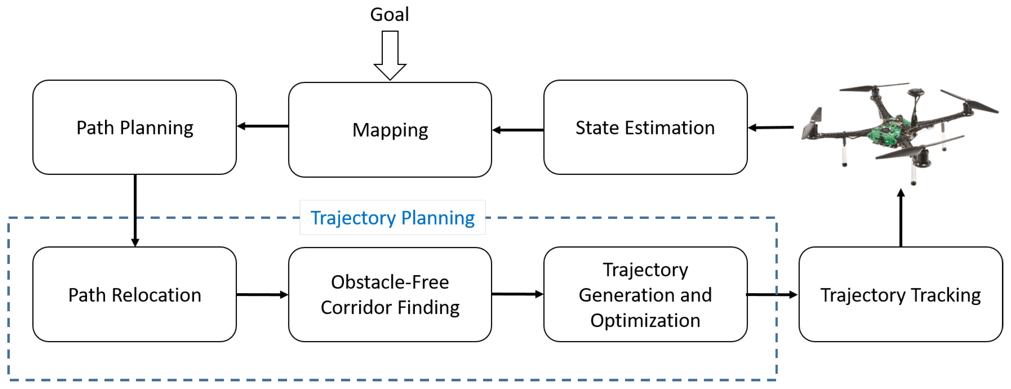
Figure 4.
Block diagram for our system.
Figure 4.
Block diagram for our system.
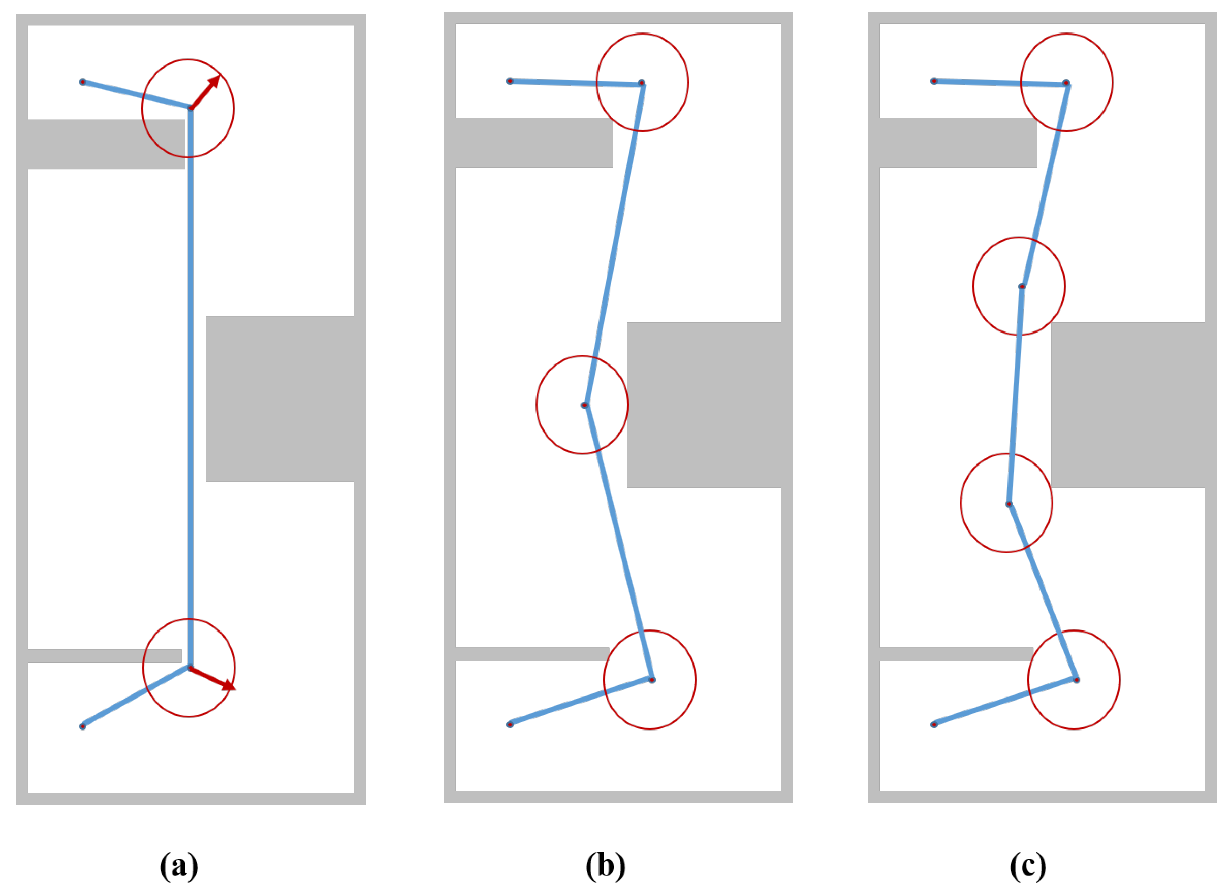
Figure 5.
Left (a): Path planned with the planning algorithm comprised of three segments with its middle segment locked among obstacles. Waypoints of the original path have been superimposed with margin spheres shown in red. Center (b): Middle segment of the planned path in (a) is bisected into two sub-segments and the new waypoint is defined at the cut point. Now we have more freedom to relocate the path. Right (c): Middle segment of the planned path in (a) is divided into three sub-segments and new waypoints are defined at cut points. We have even more freedom to relocate the path in (c).
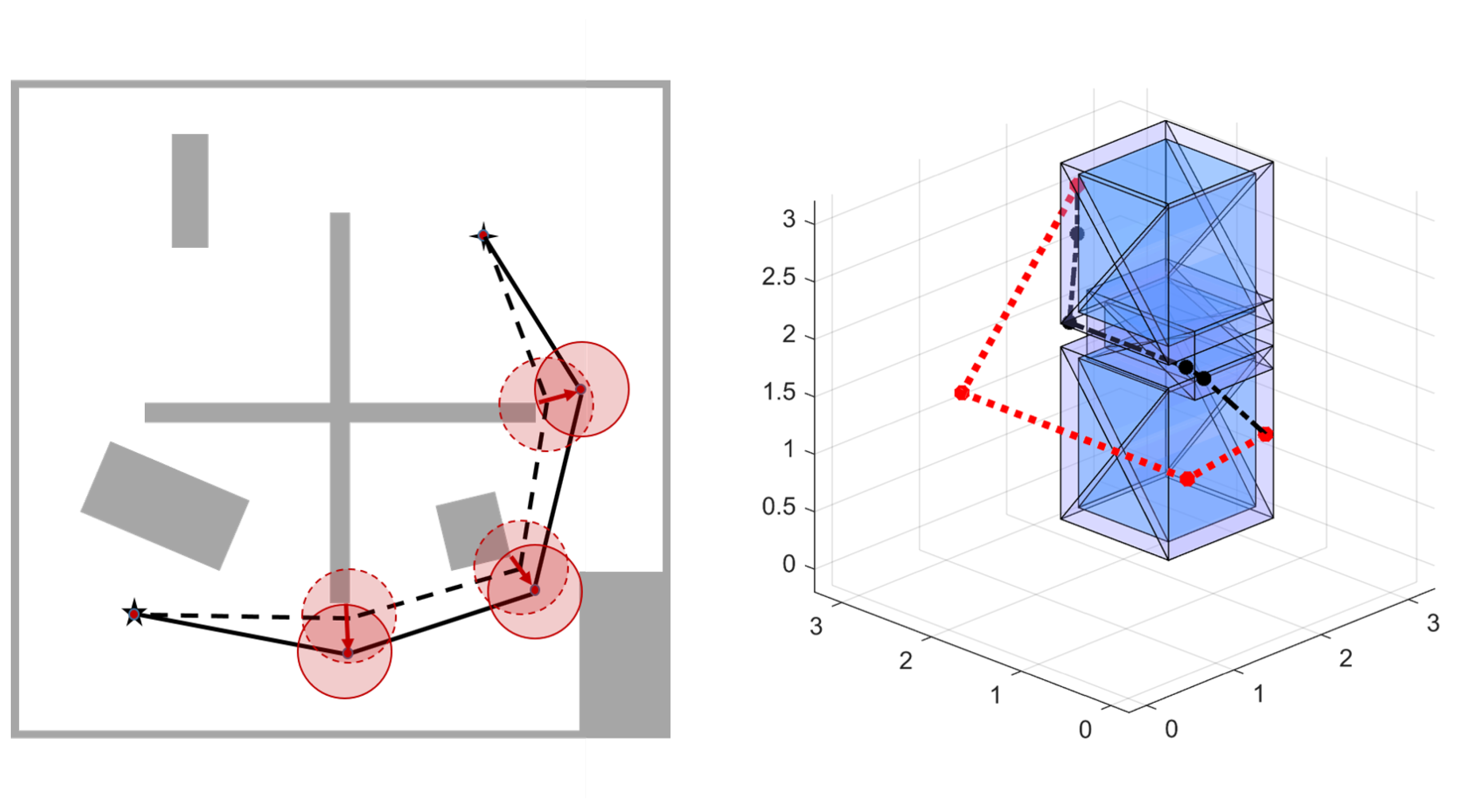
Figure 6.
Left: The Path Relocation (PR) concept in a 2D map, where obstacle space is represented with gray area. The black dotted line shows the original path planned by the planning algorithm and the black solid line shows the relocated path. Margin spheres along with relocation direction arrow are shown in red color. Right: Path relocation results in 3D map, where obstacle space is represented with blue cubes. The black dotted line show original path planned by the planning alogrithm. Red dotted line shows relocated path produced by Path Relocation (PR) step. Note the removal of extra-small segments and increase in the spacing between relocated path and obstacles.
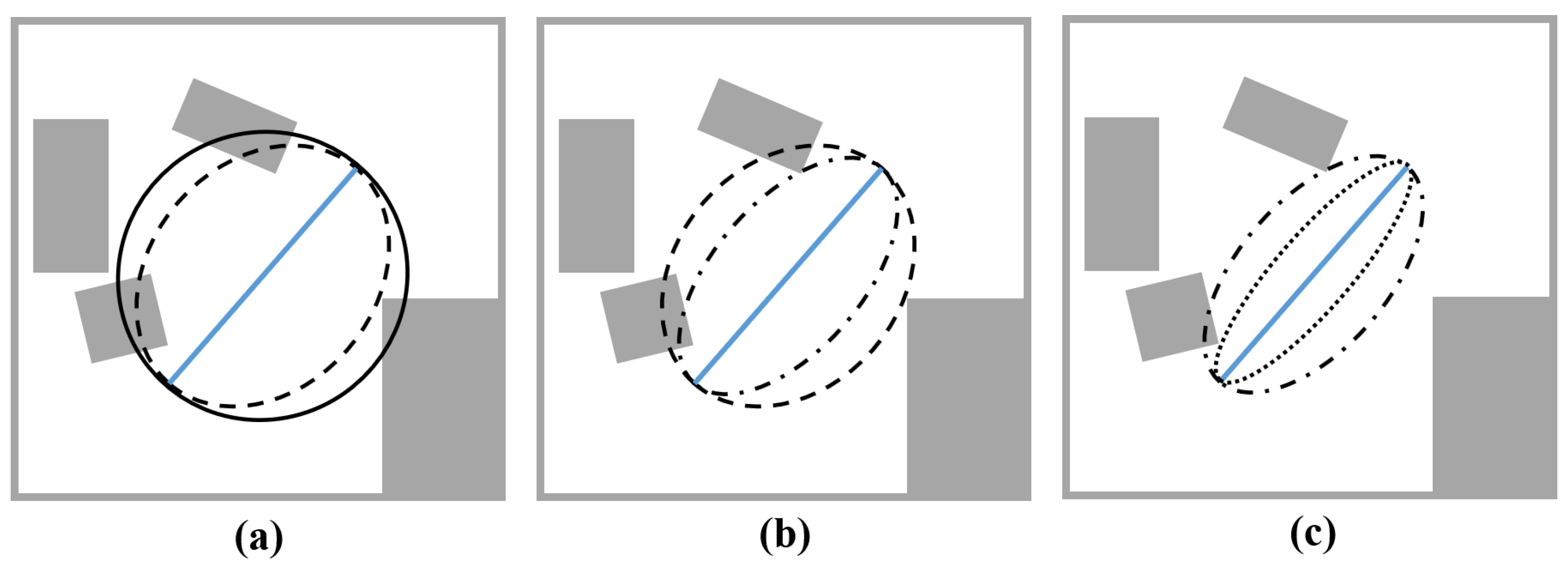
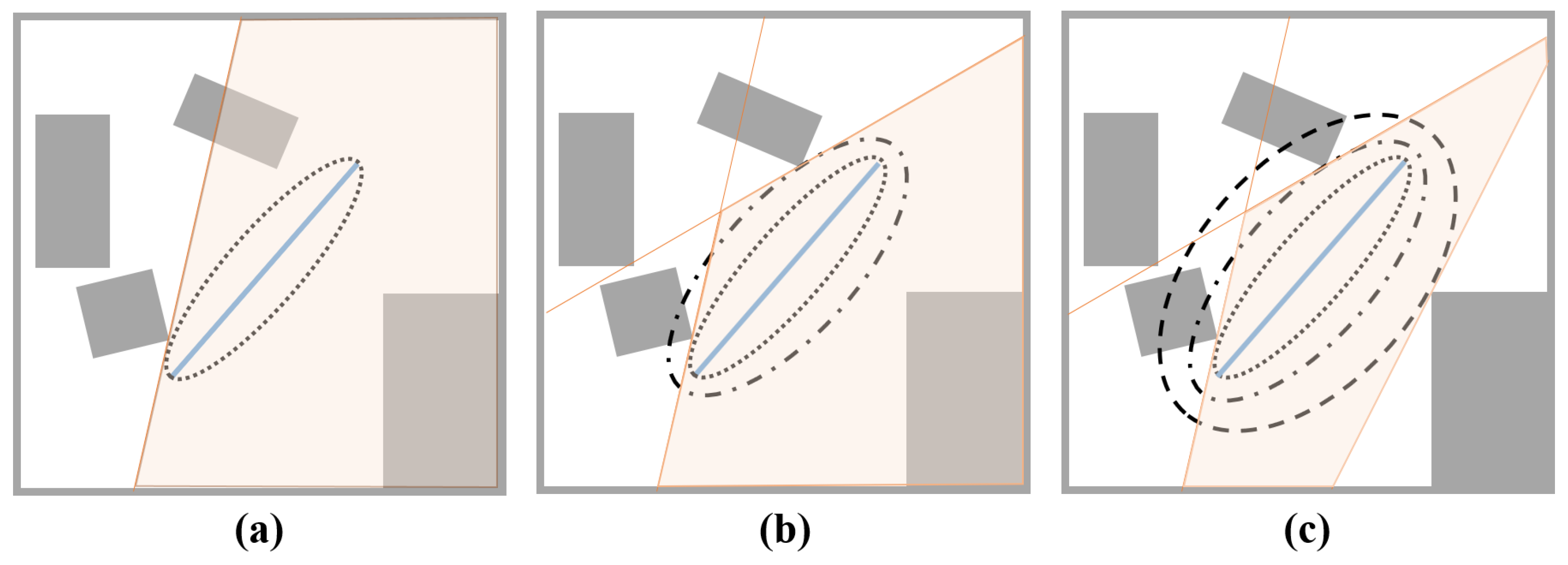
Figure 7.
Ellipsoid shrinking process shown in 2D, where grey area represents obstacle space of environment map. The blue solid line segment represents a single segment of the planned path. Left (a): We start with a black solid-line ellipsoid shown in (a). We find a point in the obstacle space that is closest to the center of the blue path segment to generate the black dashed-line ellipsoid. This completes the first iteration of ellipsoidal shrinking. Center (b): Now, we take the black dashed-line ellipsoid generated in (a) as a reference and repeat another iteration of the shrinking process to generate a black dashed-dotted-line ellipsoid. Right (c): Again, we take the black dashed-dotted-line ellipsoid generated in (b) as a reference and repeat another iteration of the ellipsoid shrinking process to generate the black dotted-line ellipsoid shown in (c). After this iteration, we may define -plane of ellipsoid.
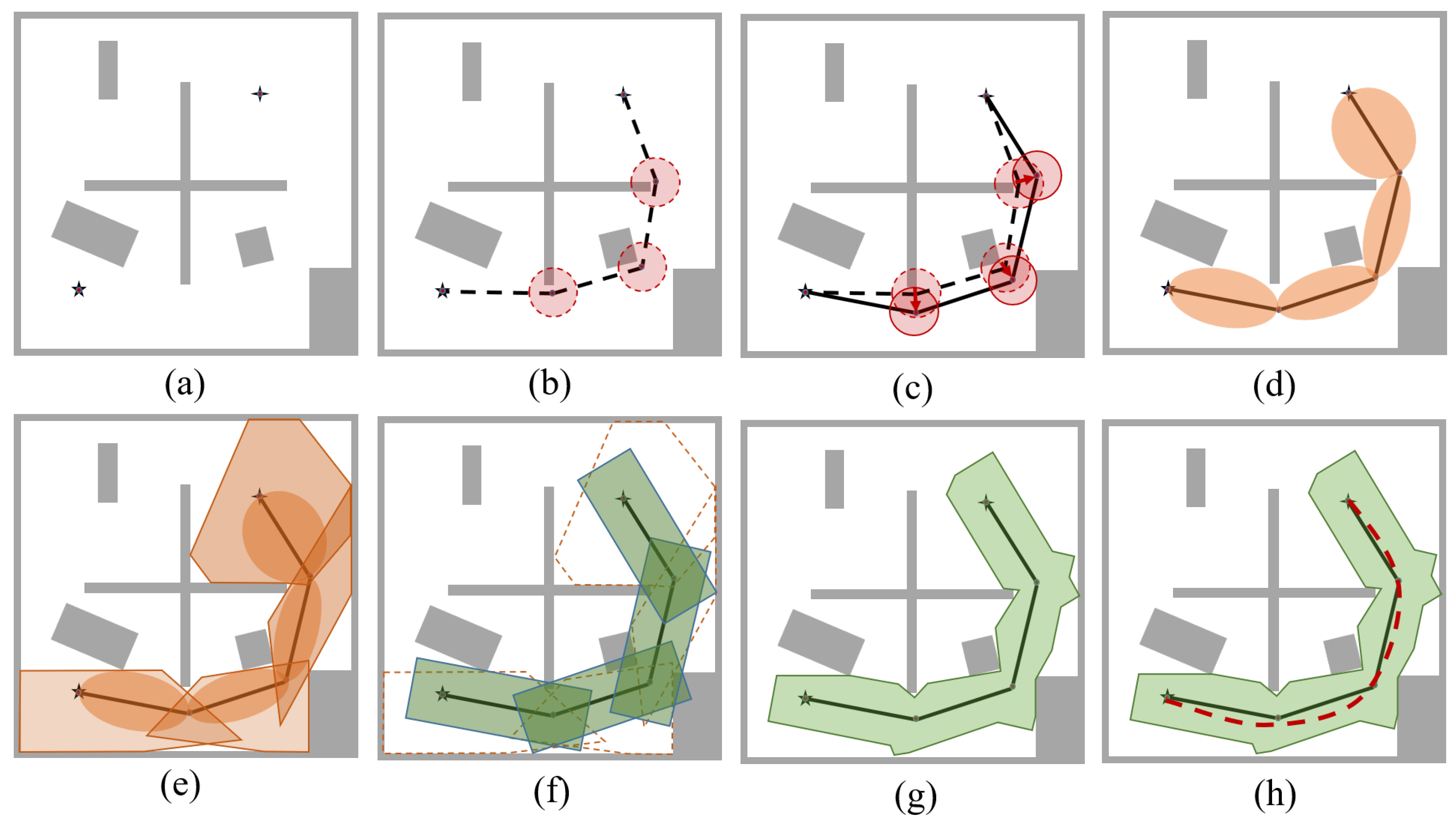
Figure 8.
Robotic motion planning process in sequence in 2D. (a) Map of the environment representing obstacles (grey areas), starting location (four-point star), and goal location (five-point star). (b) Initial path planned with planning algorithm (dotted line segments). Margin spheres are represented in red at waypoints. (c) The modified path after the application of the path relocation procedure (solid line segments). (d) Path segments with obstacle-free ellipsoids superimposed on corresponding segments. (e) Representation of polyhedra encapsulating corresponding ellipsoids (in orange color) on every path segment. (f) Cuboidal bonding of polyhedra (in green) to find tunnel-like pathway. (g) Intersection of polyhedra and cuboids to find obstacle-free corridor (OFC) represented in green. (h) Obstacle-free corridor along with optimized trajectory represented in red with dashed lines.
Figure 9.
Ellipsoidal dilation and polyhedron finding process. Orange-colored solid-lines represent the hyperplanes that we find in each iteration of the ellipsoidal dilation process. Light-shaded orange areas represent the halfspaces defined by these hyperplanes. Left (a): We start the ellipsoidal dilation process with the ellipsoid represented with dotted-line and find the first hyperplane as shown in (a). Center (b): We dilate further to find the second hyperplane, which is tangent to the ellipsoid represented with dashed-dotted-line and shown in (b). Right (c): Again, we dilate once last time to find the third hyperplane, which is tangent to the third ellipsoid (represented with dashed-line) and shown in (c). By finding the intersection of these halfspaces (defined by corresponding hyperplanes), we may form a polyhedron for the corresponding segment.
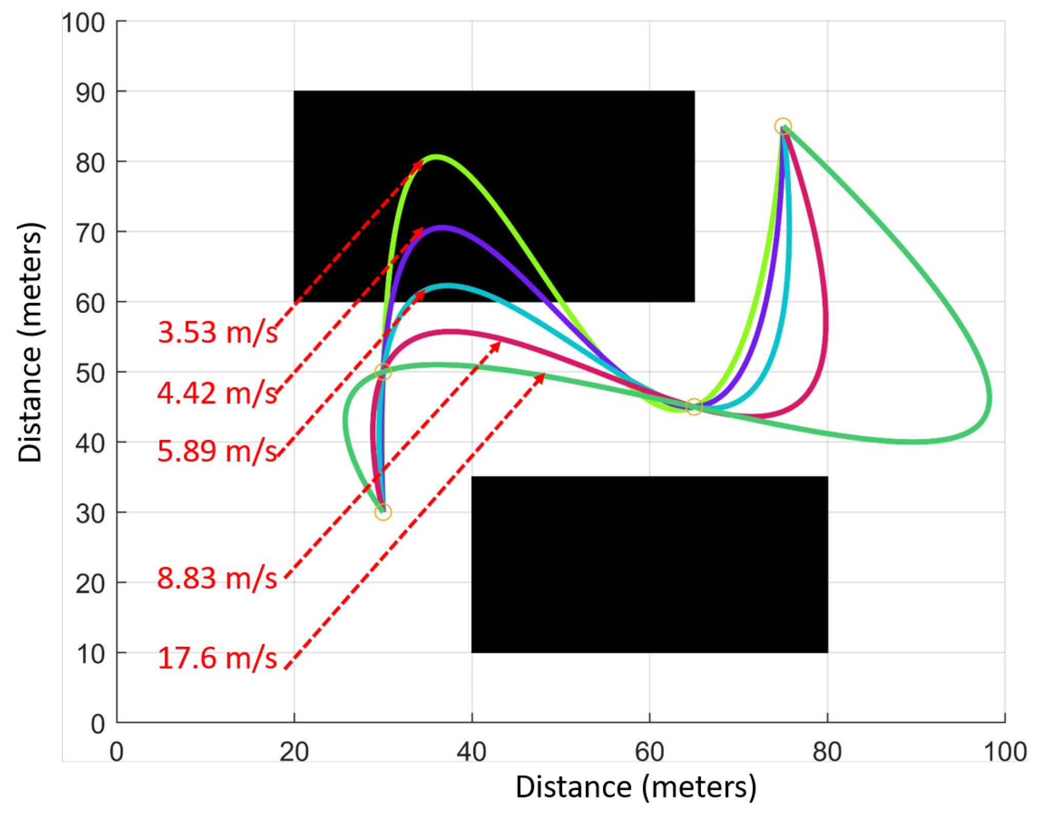
Figure 10.
Trajectory optimization problem solved with the same objective and constraints but with different segment times for the middle segment. Corresponding average vehicle velocities during the segment passage are shown in the figure.
Figure 10.
Trajectory optimization problem solved with the same objective and constraints but with different segment times for the middle segment. Corresponding average vehicle velocities during the segment passage are shown in the figure.
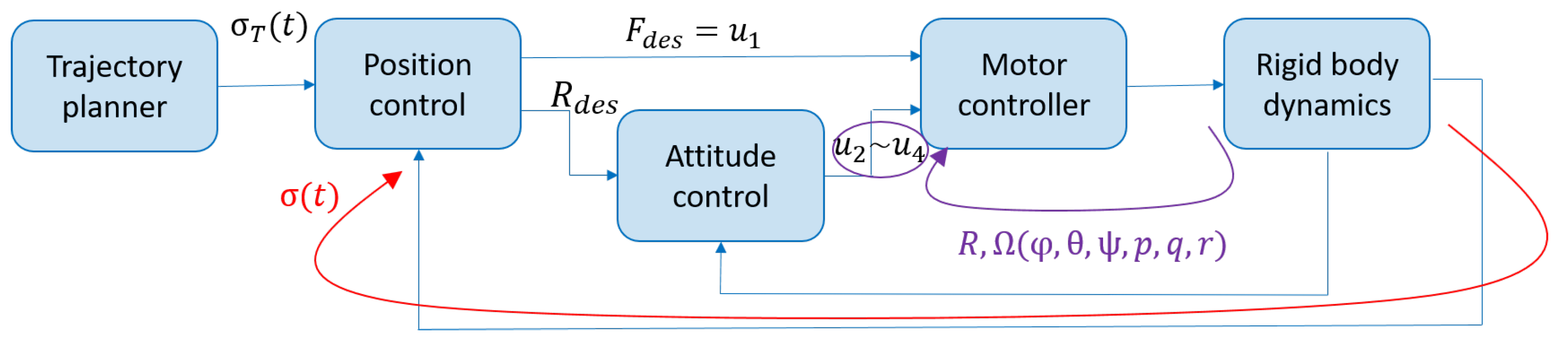
Figure 11.
Cascade control loops for position and attitude control of quadrotor. Inner loop takes commanded orientation, , as input and current attitude with angular velocities from feedback to provide control signal, , for attitude tracking. Outer loop takes desired trajectory, , as input and current trajectory from feedback to provide desired orientation, , and desired force .
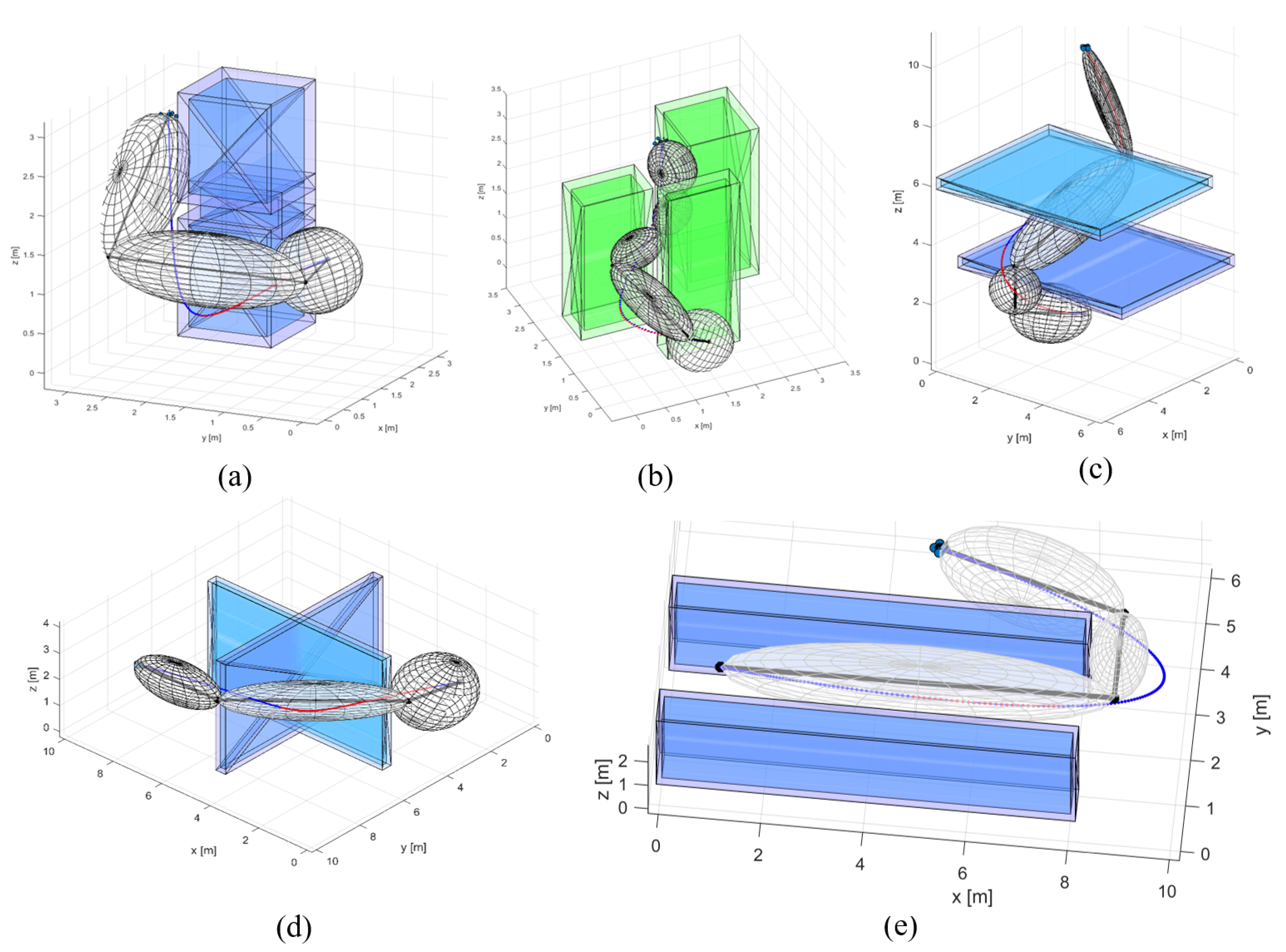
Figure 12.
Trajectories simulated with different scenarios. Optimized reference trajectories are presented in blue while trajectories tracked with a controller are presented in red. We used five different scenarios for the simulation of our navigation algorithm. Each scenario represents ellipsoids generated for Obstacle-Free Corridor (OFC) construction for corresponding path segments. Scenarios are named (a) Vertical boxes, (b) Vertical columns, (c) Multiple floors, (d) Multiple rooms, and (e) Long Corridor.
Table 1.
Execution times for different parts of our algorithm. Since the Path Relocation (PR) step is the unique feature of our algorithm, we test our system with PR and without PR.
Table 1.
Execution times for different parts of our algorithm. Since the Path Relocation (PR) step is the unique feature of our algorithm, we test our system with PR and without PR.
| | Execution Times (sec) |
|---|
| Map Scenario | Map Size | Voxel Size | Path Planning | Path Relocation | Obstacle-Free Corridor | Trajectory Optimization |
|---|
| | (m) | (cm) | JPS-3D | RRT* | PR | with PR | w/o PR | with PR | w/o PR |
|---|
| (a) Vertical Boxes | 3 × 3 × 3 | 1 × 1 × 1 | 0.242581 | 2.257435 | 0.060654 | 0.244080 | 0.346878 | 0.549249 | 0.583510 |
| (b) Vertical Columns | 3 × 3 × 3 | 2 × 2 × 2 | 0.081071 | 2.236969 | 0.069489 | 0.590176 | 0.624557 | 0.571728 | 0.604901 |
| (c) Multiple Floors | 6 × 6 × 10 | 1 × 1 × 1 | 2.891760 | 6.154565 | 0.097741 | 1.691436 | 1.700918 | 0.457560 | Failure 1 |
| (d) Multiple Rooms | 10 × 10 × 4 | 1 × 1 × 1 | 1.141364 | 1.915849 | 0.079010 | 0.594684 | 0.718829 | 0.563237 | Failure 1 |
| (e) Long Corridor | 10 × 6 × 2.5 | 1 × 1 × 1 | 1.192246 | 2.445646 | 0.073292 | 1.355371 | 2.086071 | 0.469419 | Failure 1 |
Table 2.
Control errors for different scenarios.
Table 2.
Control errors for different scenarios.
| | Trajectory Tracking Errors (m) |
|---|
| Scenario | | Position Error | Velocity Error |
|---|
| | | (X) | (Y) | (Z) | (X) | (Y) | (Z) |
|---|
| (a) Vertical Boxes | Avg | 0.0004212 | 0.0003679 | −0.000943 | −0.00011 | −0.000128 | −5.9 × |
| Std | 0.0043779 | 0.0010597 | 0.0006761 | 0.006752 | 0.001215 | 0.0014844 |
| (b) Vertical Columns | Avg | 0.0020147 | 0.0016125 | −0.002118 | −0.00012 | 0.000418 | −0.000220 |
| Std | 0.0078534 | 0.0033446 | 0.0015237 | 0.015492 | 0.006828 | 0.0042388 |
| (c) Multiple Floors | Avg | 0.0010556 | −2.6 × | −0.000627 | −3.21 × | −5.76 × | −3.62 × |
| Std | 0.0026302 | 0.0003872 | 0.0005803 | 0.002554 | 0.000284 | 0.0007287 |
| (d) Multiple Rooms | Avg | −0.000168 | 0.0003581 | −0.000636 | −0.000158 | 5.586 × | −1.09 × |
| Std | 0.0015317 | 0.0017368 | 0.0004299 | 0.001163 | 0.00131 | 0.0004918 |
| (e) Long Corridor | Avg | −5.88 × | 0.00010533 | −0.000768 | −0.000411 | −5.73 × | −3.03 × |
| Std | 0.0022831 | 0.0004938 | 0.0006614 | 0.0029307 | 0.0003791 | 0.0007432 |
Table 3.
Optimization performance of our algorithm for different scenarios with and without the Path Relocation (PR) step in trajectory planning pipeline.
Table 3.
Optimization performance of our algorithm for different scenarios with and without the Path Relocation (PR) step in trajectory planning pipeline.
| Scenario | Map Size (m) | No. of Iterations | Objective Function Value |
|---|
| w/o PR | with PR | w/o PR | with PR |
|---|
| (a) Vertical Boxes | 3 × 3 × 3 | 9 | 8 | 447.88 | 0.9492 |
| (b) Vertical Columns | 3 × 3 × 3 | 11 | 9 | 574.15 | 109.33 |
| (c) Multiple Floors | 6 × 6 × 10 | 2000 | 8 | Failure 1 | 3.1678 |
| (d) Multiple Rooms | 10 × 10 × 4 | 2000 | 8 | Failure 1 | 0.9492 |
| (e) Long Corridor | 10 × 6 × 2.5 | 2000 | 7 | Failure 1 | 1.3553 |


